Quantum phase transitions in fully connected spin models :
an entanglement perspective

Abstract

We consider a set of fully connected spins models that display first- or second-order transitions and for which we compute the ground-state entanglement in the thermodynamical limit. We analyze several entanglement measures (concurrence, Rényi entropy, and negativity), and show that, in general, discontinuous transitions lead to a jump of these quantities at the transition point. Interestingly, we also find examples where this is not the case.

I Introduction

During the last decade, the relationship between quantum phase transitions and entanglement has become an important research domain Amico et al. (2008). Although it is natural to expect some deep changes in the ground state of a system at a transition point, the real problem is to measure these variations or, in other words, to characterize the quantum state structure. In most cases, the study of an order parameter or the behavior of correlation functions is sufficient to detect and analyze a phase transition but one may wonder whether more “intrinsic” measures could be helpful. Following pioneering works in one-dimensional spin models Osborne and Nielsen (2002); Osterloh et al. (2002); Vidal et al. (2003), many studies have been devoted to this problem (see Ref. Amico et al., 2008 for a review), but only a few allow for an exact solution in the thermodynamic limit which is a key ingredient to characterize a phase transition.

The goal of this paper is to propose a class of simple, fully connected (collective) models in which ground-state entanglement properties can be studied in details. These models, in which degrees of freedom (spins 1/2) mutually interact, can be seen as generalizations of the Lipkin-Meshkov-Glick model Lipkin et al. (1965); Meshkov et al. (1965); Glick et al. (1965) for which most entanglement features are now well known Vidal et al. (2004a, b, c); Dusuel and Vidal (2004); Latorre et al. (2005); Dusuel and Vidal (2005); Unanyan et al. (2005); Barthel et al. (2006); Vidal (2006); Vidal et al. (2007); Morrison and Parkins (2008); Cui (2008); Orús et al. (2008); Caneva et al. (2008); Ma et al. (2009); Wichterich et al. (2010). The main reason for introducing these collective systems is that they not only allow us to study a second-order phase transition as in the Lipkin-Meshkov-Glick model, but also allow the study of first-order transitions. As surprising as it may seem, although “collective” may be thought to lead to a pure mean-field behavior, we will see that the is deeply entangled. Furthermore, although it might be naively expected that entanglement measures will simply display jumps at first-order transitions, we will show that this does not hold for one of the models, the spectral properties of which show some similarities with those of a system exhibiting a second-order transition.

The study of these collective systems is also motivated by the fact that they are much simpler to analyze than their nearest-neighbor counterparts on a finite-dimensional lattice. Indeed, most entanglement measures rely on a multi-partition of the microscopic degrees of freedom. For instance, the concurrence Wootters (1998) is obtained by separating a system of $N$ spins into two parts (of sizes $N-2$ and $2$), the Rényi entropy is obtained by splitting it into two parts of arbitrary sizes ($N-L$ and $L$), a tri-partition is required to compute the negativity Vidal and Werner (2002) of a mixed state, etc. Thus, the main problem often consists of computing reduced density matrices for a given partition. In the models studied below, this crucial step can be achieved since the original spin problem can be mapped onto a quadratic bosonic Hamiltonian.

The structure of this paper is the following. In Sec. II, we introduce a family of models and compute their low-energy spectrum (ground-state energy and gap). This allows us to determine their phase diagram and characterize the quantum phase transitions. Analytical expressions are obtained in the thermodynamical limit and compared with exact diagonalization results. In Sec. III, we discuss the ground-state entanglement by focusing on three different measures : the concurrence, the Rényi entropy, and the negativity, which rely on a one-mode, two-mode, and three-mode description of the bosonic Hamiltonian, respectively. Once again, exact results in the thermodynamical limit are compared to numerical data for a representative set of parameters.

II Models and quantum phase transitions

II.1 Hamiltonians

We consider a system made of $N$ spins 1/2 whose Hamiltonian reads

$$H=-N\left[\cos\omega\left(\frac{S_{x}}{S}\right)^{m}+K_{m,n}\sin\omega\left(\frac{S_{z}}{S}\right)^{n}\right].$$ (1)

In the above equation, $S_{\alpha}=\sum_{j=1}^{N}\sigma_{j}^{\alpha}/2$ are total spin operators along the $\alpha=x$, $y$, $z$ direction, with $\sigma_{j}^{\alpha}$ being the usual Pauli matrix at site $j$ and $S=N/2$ denotes the maximum spin value. This class of models is defined by the non-negative integer parameters $(m,n)$. In what follows, we shall refer to a model with given values of $m$ and $n$ as the $(m,n)$ model.

Without loss of generality, we shall restrict ourselves to $m\geqslant n\geqslant 1$. We furthermore exclude the trivial case $m=n=1$, since it describes a large spin in a magnetic field, and only displays a crossover, but no quantum phase transition. The $(2,1)$ model is a collective version of the transverse-field Ising model, known as the Lipkin-Meshkov-Glick model Lipkin et al. (1965); Meshkov et al. (1965); Glick et al. (1965). The $(m>2,1)$ models are multispin generalizations of such a model. The $(2,2)$ model can be seen as a collective version of the quantum compass model Kugel and Khomskii (1982). Note that, in two dimensions, the latter is dual to the Xu-Moore model Xu and Moore (2004, 2005); Nussinov and Fradkin (2005), but the collective version of the Xu-Moore model, namely, the $(4,1)$ model, is not dual to the $(2,2)$ model (in fact, as will be seen below, the latter two models have rather different properties).

As we shall see, all models under consideration exhibit a quantum phase transition when the control parameter $\omega\in[0,\pi/2]$ is varied. This quantum phase transition occurs at $\omega=\pi/4$, provided one imposes $K_{m,n}$ to take the following value Maritan et al. (1984):

$$K_{2,1} = 2,$$ (2)

$$K_{m>2,1} = \frac{m^{m/2}(m-2)^{m/2-1}}{(m-1)^{m-1}},$$ (3)

$$K_{m\geqslant 2,n\geqslant 2} = 1.$$ (4)

These values can be found easily (see Sec. II.2.2 for details).

Finally, let us note that all Hamiltonians preserve the magnitude of the total spin, i. e., $[H,\boldsymbol{S}^{2}]=0$. When $m$ ($n$) is even, the Hamiltonian furthermore has a spin-flip symmetry since it commutes with $\prod_{j}\sigma_{j}^{z}$ ($\prod_{j}\sigma_{j}^{x}$).

II.2 Quantum phase transitions

II.2.1 Numerical spectra

Physically, the quantum phase transition stems from the competition between the ferromagnetic $m$-spin interaction in the $x$ direction and the ferromagnetic $n$-spin interaction in the $z$ direction if $n>1$, or magnetic field in the $z$ direction if $n=1$.

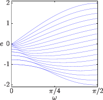
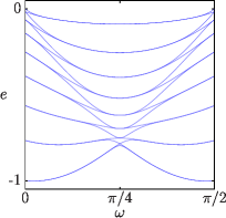
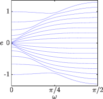
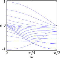
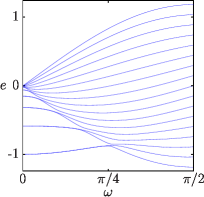
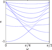
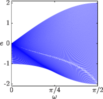
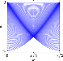
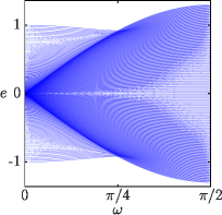
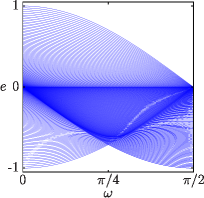
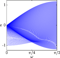
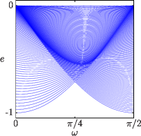
A numerical study provides an idea about the phase transitions of the various models. Such a study can be performed for rather large number of spins since, as already mentioned, the Hamiltonians commute with $\boldsymbol{S}^{2}$. The collective and ferromagnetic nature of the interactions implies that one can focus on the maximum spin sector $S=N/2$ (of dimension $N+1$) where the ground state is found. The energies per spin $e$ of six different models are shown in Figs. 1 and 2, for $N=16$ and $N=256$ respectively. From the evolution of the full spectra between these two figures, one can infer the behavior of the various models in the thermodynamical limit.

The $(2,1)$ model displays a collapse of levels onto the ground state, at the transition point $\omega=\pi/4$, but the ground-state energy displays no cusp. From these features, the quantum phase transition is likely to be of second order. All other models (except the $(2,2)$ model) have avoided level crossings, which tend to become true level crossings in the thermodynamical limit. In particular, the ground-state energy has a cusp, and the transition is of first order. Note that, in Fig. 2, the darker regions are those where one finds many levels (which are finite-size precursors of singularities in the density of states in the thermodynamical limit). But, contrary to what happens for the $(2,1)$ model Ribeiro et al. (2007, 2008), these regions do not touch the ground-state energy at the transition. This is, however, not true for the $(2,2)$ model, which displays both a collapse of levels onto the ground state as well as a cusp in the ground-state energy. From the second feature, one concludes that the transition is first order, although the first feature is reminiscent of a second-order quantum phase transition. Let us stress that the $(2,2)$ model is trivially integrable at the transition point, since its Hamiltonian reads $H=-\frac{2\sqrt{2}}{N}(S^{2}-S_{y}^{2})$, where $S^{2}=(N/2)(N/2+1)$. This additional symmetry ($[H,S_{y}]=0$) is responsible for the presence of non-avoided level crossings at the transition point, even at finite $N$. Actually, all these models are exactly solvable, but not in such a trivial way Pan and Draayer (1999); Links et al. (2003); Ortiz et al. (2005).

It is this variety of behaviors displayed by the different models that motivates the study of entanglement measures and their sensitivity to the characteristics of the quantum phase transition. Before turning to this, we shall, however, provide analytical results for the low-energy spectrum, which will allow us to introduce the basic techniques needed to perform analytical computations of entanglement measures.

Figure 1: (Color online) Spectra (energies per spin) of six models as a function of the control parameter $\omega$, for a system of $N=16$ spins, in the maximum spin sector $S=N/2$. Left (right): $n=1$ ($n=2$). From top to bottom : $m=2$, $m=3$, and $m=4$.

Figure 2: (Color online) Spectra (energies per spin) of six models as a function of the control parameter $\omega$, for a system of $N=256$ spins, in the maximum spin sector $S=N/2$. Left (right): $n=1$ ($n=2$). From top to bottom : $m=2$, $m=3$, and $m=4$.

II.2.2 Ground-state energy

Since a large spin behaves classically, a classical analysis is expected to provide exact results for the ground-state energy of the collective models in the thermodynamical limit. We are therefore led to substitute the spin operators by their expectation values, namely

$$\big{(}\left\langle S_{x}\right\rangle,\left\langle S_{y}\right\rangle,\left\langle S_{z}\right\rangle\big{)}=\frac{N}{2}\left(\sin\theta\cos\phi,\sin\theta\sin\phi,\cos\theta\right),$$ (5)

where $\theta\in\left[0,\pi\right]$ and $\phi\in\left[0,2\pi\right[$ are the usual angles of spherical coordinates. They are the variational parameters that will be tuned to minimize the associated classical energy per spin

$$e(\theta,\phi)=-\cos\omega(\sin\theta\cos\phi)^{m}-K_{m,n}\sin\omega(\cos\theta)^{n}.$$ (6)

When $m>n=1$, the analysis follows the mean-field calculation of Ref. Maritan et al., 1984 [see also Refs. Botet and Jullien, 1983; Dusuel and Vidal, 2005 for the $(2,1)$ model]. At “large” $\omega$ (close to $\pi/2$), the state $(\theta_{0}=0,\phi)$ is the only minimum, with energy $e(0,\phi)=-K_{m,1}\sin\omega$. At “small” $\omega$ (close to $0$), $\phi_{0}=0$ ($\phi_{0}=0$ or $\pi$) when $m$ is odd (even), and the angle $\theta_{0}$ minimizing the energy satisfies $m\cos\theta_{0}\sin^{m-2}\theta_{0}=K_{m,1}\tan\omega$. Requiring that the transition take place at $\omega=\pi/4$, one is led to solve the following system of equations:

$$K_{m,1} = m\cos\theta_{0}^{*}\sin^{m-2}\theta_{0}^{*},$$ (7)

$$K_{m,1} = \sin^{m}\theta_{0}^{*}+K_{m,1}\cos\theta_{0}^{*},$$ (8)

where the second equation stems from the continuity of $e$ at the transition, and $\theta_{0}^{*}$ is the value of $\theta_{0}$ at the transition, in the small-$\omega$ phase. The solution of this system yields Eqs. (2) and (3), as well as $\cos\theta_{0}^{*}=\frac{1}{m-1}$. It is therefore clear that, except for the $(2,1)$ model, $\theta_{0}$ is discontinuous at the transition, which is thus of first order for all $(m>2,1)$ models.

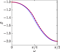
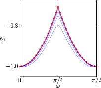
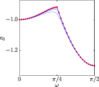
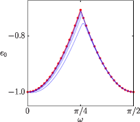
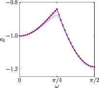
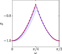
For the $(2,1)$ model, the transition is of second order (see e. g. Ref Botet and Jullien, 1983), as can be seen from the discontinuity of the second derivative $\frac{\partial^{2}e}{\partial\omega^{2}}$ which jumps from the value $-3\sqrt{2}$ at $\omega=(\pi/4)^{-}$ to $\sqrt{2}$ at $\omega=(\pi/4)^{+}$. The large-$\omega$ phase is a symmetric phase with a non-degenerate ground state, while the small-$\omega$ phase is a broken phase with a doubly-degenerate ground state, the broken symmetry being the parity $S_{x}\leftrightarrow-S_{x}$. The validity of the classical analysis can be assessed in Fig. 3 where numerical data can be seen to converge to the classical result.

When $m\geqslant n\geqslant 2$, one can proceed in the same way. One finds that the transitions are all of first-order nature, that Eq. (4) has to hold in order to have a transition at $\omega=\pi/4$, and that the angles $\theta_{0}$ and $\phi_{0}$ take the following values

$$\omega\leqslant\pi/4$$

()

() any

(9)

The values in parentheses are other possible values depending on the parity of $m$ and $n$. For $\omega\leqslant\pi/4$, the states $(\pi/2,0)$ and $(\pi/2,\pi)$ are degenerate when $m$ is even, whereas for $\omega\geqslant\pi/4$, the states $(0,\phi_{0})$ and $(\pi,\phi_{0})$ are degenerate when $n$ is even. The degeneracies are already predictable from Fig. 1, and the validity of the classical results can again be checked in Fig. 3.

Figure 3: (Color online) Ground-state energy per spin $e_{0}$ of six models as a function of $\omega$, for $N=16$, $32$, $64$, $128$, $256$ and in the thermodynamical limit (red thick line with dots). Left (right): $n=1$ ($n=2$). From top to bottom : $m=2$, $m=3$, and $m=4$.

II.2.3 Gap

In order to conclude the analysis of the spectrum and of the quantum phase transition of these models, let us now turn to the computation of the gap, in the maximum spin sector $S=N/2$. We follow the procedure described in Refs. Dusuel and Vidal (2004, 2005) and refer the reader to these references for details. As a first step, we perform a rotation around the $y$-axis, in order to bring the $z$-axis along the classical magnetization direction

$$\begin{pmatrix}S_{x}\\ S_{y}\\ S_{z}\end{pmatrix}=\begin{pmatrix}\cos\theta_{0}&0&\sin\theta_{0}\\ 0&1&0\\ -\sin\theta_{0}&0&\cos\theta_{0}\end{pmatrix}\begin{pmatrix}\widetilde{S}_{x}\\ \widetilde{S}_{y}\\ \widetilde{S}_{z}\end{pmatrix}.$$ (10)

Figure 4: (Color online) Gaps to the first two excited states of six models as a function of $\omega$, for $N=16$, $32$, $64$, $128$, $256$ and in the thermodynamical limit (red thick line with dots). Left (right): $n=1$ ($n=2$). From top to bottom : $m=2$, $m=3$, and $m=4$.

Next, we make use of the bosonic Holstein-Primakoff representation of the rotated spin operators Holstein and Primakoff (1940)

$$\widetilde{S}_{z}=\frac{N}{2}-a^{\dagger}a\,\mbox{ and }\,\widetilde{S}_{+}=\left(N-a^{\dagger}a\right)^{1/2}a={\widetilde{S}_{-}}^{\dagger},$$ (11)

where $\widetilde{S}_{\pm}=\widetilde{S}_{x}\pm\mathrm{i}\widetilde{S}_{y}$ and the $a$ operator is a bosonic annihilation operator, satisfying $\left[a,a^{\dagger}\right]=1$. As we shall only focus on the thermodynamical limit, it will be sufficient to keep terms of order $N^{1}$ and $N^{0}$ in the Hamiltonian, neglecting all terms that go to zero as $N\to\infty$, (assuming a finite number $a^{\dagger}a$ of bosons). For example, in the large-$\omega$ phase, one can write $S_{x}=\widetilde{S}_{x}=N^{1/2}(a^{\dagger}+a)/2$. Note that no term of order $\sqrt{N}$ appears, thanks to the rotation we have performed. The Hamiltonian then reads

$$H=Ne_{0}+\gamma+\delta\,a^{\dagger}a+\gamma\left({a^{\dagger}}^{2}+{a^{\phantom{\dagger}\!\!\!}}^{2}\right),$$ (12)

where $e_{0}$, $\gamma$ and $\delta$ have the following expressions (the value of $\theta_{0}$ has been given in Sec. II.2.2)

$$e_{0} = -\cos\omega(\sin\theta_{0})^{m}-K_{m,n}\sin\omega(\cos\theta_{0})^{n},$$ (13)

$$\gamma = -\frac{1}{2}\big{[}m(m-1)\cos\omega(\sin\theta_{0})^{m-2}(\cos\theta_{0})^{2}$$ (14)

$$+n(n-1)K_{m,n}\sin\omega(\cos\theta_{0})^{n-2}(\sin\theta_{0})^{2}\big{]},$$

$$\delta = 2\big{[}m\cos\omega(\sin\theta_{0})^{m}+nK_{m,n}\sin\omega(\cos\theta_{0})^{n}\big{]}$$ (15)

$$+2\gamma.$$

Note that $e_{0}$ is simply the minimum of the classical ground-state energy (6).

Such a quadratic Hamiltonian is diagonalized via a Bogoliubov transformation

$$a=\cosh(\Theta/2)b+\sinh(\Theta/2)b^{\dagger},$$ (16)

where $b$ is a bosonic annihilation operator, satisfying $\left[b,b^{\dagger}\right]=1$. The value of $\Theta$ diagonalizing the Hamiltonian satisfies $\tanh\Theta=\varepsilon=-2\gamma/\delta$. With these notations,

$$H=Ne_{0}+\gamma+\frac{\delta}{2}\left(\sqrt{1-\varepsilon^{2}}-1\right)+\Delta\,b^{\dagger}b,$$ (17)

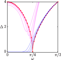
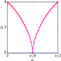
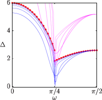
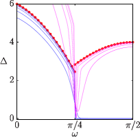
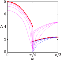
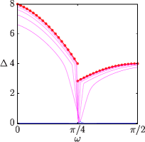
where the gap is $\Delta=\delta\sqrt{1-\varepsilon^{2}}$. Let us emphasize that $\Delta$ is the gap above the possibly-degenerate ground state, but does not capture the energy splitting between the ground states if they are degenerate. We compare the spectrum of Eq. (17) with numerics in Fig. 4 for the gap to the first and second excited states, so we get at least one (and possibly two) nonzero value in the thermodynamical limit. The relevance of this simple “spin-wave”-like approach can be appreciated.

III Entanglement measures

III.1 Technical prerequisite

We shall now compute three entanglement measures, namely, the concurrence, the entanglement entropy, and the logarithmic negativity. These measures have already been computed for the $(2,1)$ model in Refs. Dusuel and Vidal, 2004, 2005; Latorre et al., 2005; Barthel et al., 2006; Vidal et al., 2007; Wichterich et al., 2010. As can be inferred from these works, the analytical computations require to write the spin operators as the sum of one, two or three spin operators, for the concurrence, entanglement entropy and negativity respectively. Then, one should use the Holstein-Primakoff representation. The necessary steps for the computation of the concurrence have already been performed in Sec. II.2.3, but let us give the key ingredients that are useful to obtain the other entanglement measures.

The very first step is to perform the rotation (10). Then, one splits the system into $p$ subsystems, so that the the spin operators read as $\widetilde{S}_{\alpha}=\sum_{i=1}^{p}\widetilde{S}_{\alpha}^{(i)}$, where $\alpha=x$, $y$ or $z$. Depending on the entanglement measure one wishes to compute, one has $p=1$, $2$, or $3$. One then introduces $p$ bosonic operators $a_{i}$ and their conjugates $a_{i}^{\dagger}$ for each subsystem. Denoting the number of spins of each subsystem by $N_{i}$, with $\sum_{i=1}^{p}N_{i}=N$, the $p$ Holstein-Primakoff representations read as

$$\widetilde{S}_{z}^{(i)}=\frac{N_{i}}{2}-a_{i}^{\dagger}a_{i}\,\mbox{ and }\,\widetilde{S}_{+}^{(i)}=\left(N_{i}-a_{i}^{\dagger}a_{i}\right)^{1/2}a_{i}.$$ (18)

One can then insert these expressions in the Hamiltonian, expand all operators and keep terms of order $N^{1}$ and $N^{0}$, neglecting contributions that vanish in the thermodynamical limit. After simple algebra, one gets a quadratic Hamiltonian

$$H=Ne_{0}+\gamma+\delta\sum_{i=1}^{p}a_{i}^{\dagger}a_{i}+\gamma\sum_{k,l=1}^{p}\sqrt{\tau_{k}\tau_{l}}\big{(}a_{k}^{\dagger}a_{l}^{\dagger}+\mbox{H.c.}\big{)},$$ (19)

where $e_{0}$, $\gamma$, and $\delta$ are given in Eqs. (13)-(15) and where $\tau_{i}=N_{i}/N$. Let us note that, to obtain this precise quadratic form, with only diagonal boson-conserving terms, one must get rid of terms of the form $a_{k}^{\dagger}a_{l}$ with $k\neq l$. To this end, one should use the relation $\sum_{\alpha}\widetilde{S}_{\alpha}^{2}=S(S+1)$, written in the bosonic language, namely,

$$\sum_{k\neq l}\sqrt{\tau_{k}\tau_{l}}\big{(}a_{k}^{\dagger}a_{l}+\mbox{H.c.}\big{)}=2\sum_{i}(1-\tau_{i})a_{i}^{\dagger}a_{i}.$$ (20)

Of course, Eq. (19) yields Eq. (12) when only one bosonic mode is considered.

In the three subsections that follow, we shall give a minimal amount of computational details, knowing that these can already be found in the literature.

III.2 Concurrence

The concurrence $C$ measures the entanglement between two spins half, these spins being in either a pure or a mixed state Wootters (1998). Here, we are interested in quantifying the entanglement between any two spins, the others being traced over. Finding the concurrence amounts to computing the entries of the reduced density matrix, which can be done easily for symmetric states Wang and Mølmer (2002). However, except in the case of systems possessing a spin-flip symmetry, finding a simple analytical formula for the concurrence is not such an easy task Vidal (2006). Although we have no formal proof, we have checked numerically for finite-size systems and a couple of values of $m$ and $n$ (even when $m$ and $n$ are odd so that there is no spin-flip symmetry), that the rescaled concurrence $C_{\mathrm{R}}$ could be simply expressed as

$$C_{\mathrm{R}}=(N-1)C=1-\frac{4\langle S_{y}^{2}\rangle}{N}.$$ (21)

This rescaling is needed here because each spin shares entanglement with its $N-1$ “neighbors” Vidal et al. (2004a). Thanks to the Holstein-Primakoff representation (11) and to the Bogoliubov diagonalization of the associated Hamiltonian (16), one can show Dusuel and Vidal (2005) that in the thermodynamical limit

$$\alpha=\lim_{N\to\infty}\frac{4\langle S_{y}^{2}\rangle}{N}=\sqrt{\frac{1-\varepsilon}{1+\varepsilon}},$$ (22)

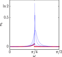
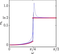
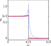
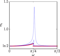
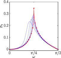
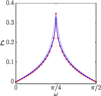
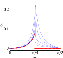
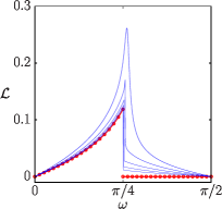
where $\varepsilon$ is given just before Eq. (17). Figure 5 displays numerical results for increasing system sizes which clearly converge toward the expression computed above in the thermodynamical limit.

Figure 5: (Color online) Concurrence of six models as a function of $\omega$, for $N=16$, $32$, $64$, $128$, $256$ and in the thermodynamical limit (red thick line with dots). Left (right): $n=1$ ($n=2$). From top to bottom : $m=2$, $m=3$, and $m=4$.

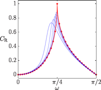
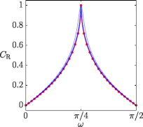
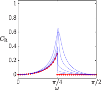
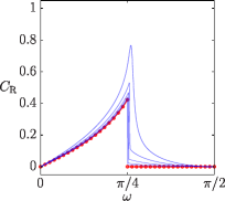
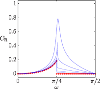
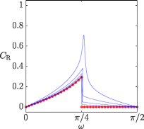
As can be inferred from this figure, the concurrence is cusped but continuous at the second-order quantum phase transition for the $(2,1)$ model, while it displays a jump at the first-order transition of the $(m,n)$ models, except for the $(2,2)$ model where it shows a cusp and is continuous. The spectral peculiarities of the latter, which have been discussed in Sec. II.2.1, do not lead to a discontinuous concurrence. It therefore seems, in this very special case, that an entanglement measure such as the concurrence is more sensitive to the “level collapse” on the ground state (Anderson’s tower structure), than to the level crossing, when both effects are present. We shall show that this conclusion remains valid for the other entanglement measures we have calculated, starting with the entanglement entropy.

III.3 Entanglement entropy

The ground-state entanglement between two complementary subsystems $\mathcal{A}$ and $\mathcal{B}$ can be quantified by the Rényi entropy, defined by

$$\mathcal{E}_{q}=\frac{1}{1-q}\ln\left[\mathrm{Tr}\left({\rho_{\mathcal{A}}}^{q}\right)\right].$$ (23)

Figure 6: (Color online) Von Neumann entanglement entropy of six models as a function of $\omega$, for $N=16$, $32$, $64$, $128$, $256$ and in the thermodynamical limit (red thick line with dots). In all cases, the system is separated in two parts of equal sizes $N_{1}=N_{2}=N/2$. Left (right): $n=1$ ($n=2$). From top to bottom : $m=2$, $m=3$, and $m=4$.

In the above equation, $\rho_{\mathcal{A}}=\mathrm{Tr}_{\mathcal{B}}\rho$ is the reduced density matrix of subsystem $\mathcal{A}$ ($\rho$ is the ground-state density matrix) and $q$ is a positive number. In the limit $q\to 1$, one recovers the usual von Neumann entropy, namely $\mathcal{E}=\lim_{q\to 1}\mathcal{E}_{q}=-\mathrm{Tr}[\rho_{\mathcal{A}}\ln\rho_{\mathcal{A}}]$. The technique for computing $\rho_{\mathcal{A}}$ has been exposed in Refs. Barthel et al., 2006; Vidal et al., 2007. To use this method one simply needs the Bogoliubov transformation which diagonalizes the Hamiltonian (19) for $p=2$ given in Appendix A. In summary, for subsystems $\mathcal{A}$ and $\mathcal{B}$ of sizes $N_{\mathcal{A}}=\tau N$ and $N_{\mathcal{B}}=(1-\tau)N$, one has (in the thermodynamical limit and in an appropriate basis)

$$\rho_{\mathcal{A}} = \frac{2}{\mu+1}\exp\left[-\ln\left(\frac{\mu+1}{\mu-1}\right)c^{\dagger}c\right],\quad\mbox{with}$$ (24)

$$\mu = \sqrt{[\tau+(1-\tau)/\alpha][(1-\tau)+\tau/\alpha]},$$ (25)

where $c$ and $c^{\dagger}$ are bosonic annihilation and creation operators and where $\alpha$ has been defined in Eq. (22). It is then straightforward to compute the Rényi entropy

$$\mathcal{E}_{q}=\frac{1}{1-q}\Big{\{}q\ln 2-\ln\big{[}(\mu+1)^{q}-(\mu-1)^{q}\big{]}\Big{\}},$$ (26)

as well as the von Neumann entropy

$$\mathcal{E}=\frac{\mu+1}{2}\ln\left(\frac{\mu+1}{2}\right)-\frac{\mu-1}{2}\ln\left(\frac{\mu-1}{2}\right).$$ (27)

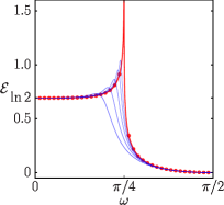
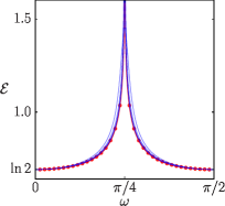
We have computed the latter numerically. As can be seen in Fig. 6, when the system size grows, the numerical results converge to the analytical expressions obtained above (to which one must in fact add a term $\ln 2$ when the ground state is two-fold degenerate).

One can furthermore see that similar conclusions to those for the concurrence can be drawn here. Indeed, the von Neumann entropy of the $(2,2)$ model diverges at the first-order transition point, like the entropy of the $(2,1)$ model but contrary to the entropy of all other models which is finite but discontinuous at the transition. In fact, the entropies of the $(2,2)$ model and of the $(2,1)$ model diverge logarithmically at the transition, as $(1/2)\ln N$ and $(1/6)\ln N$, respectively (see Refs. Latorre et al., 2005; Barthel et al., 2006). So, once again, from an entanglement perspective, the peculiar first-order transition of the $(2,2)$ model looks like a second-order transition.

III.4 Logarithmic negativity

As a final study of the ground-state entanglement properties of our class of models, let us compute the logarithmic negativity Vidal and Werner (2002). This quantity, which quantifies the entanglement between any two subsystems (in a mixed or in a pure state), was already worked out for the $(2,1)$ model Wichterich et al. (2010) and is obtained as follows. The system is divided into three subsystems $\mathcal{A}$, $\mathcal{B}$ and $\mathcal{C}$ of respective sizes $N_{1}$, $N_{2}$ and $N_{3}$. One then traces the ground-state density matrix over one of the subsystems, say $\mathcal{B}$, to obtain the reduced density matrix $\rho_{\mathcal{AC}}=\mathrm{Tr}_{\mathcal{B}}\rho$. The logarithmic negativity $\mathcal{L}$ is defined as

$$\mathcal{L}=\ln\mathrm{Tr}\left[\sqrt{\left(\rho_{\!\mathcal{AC}}^{\,\,\mathrm{T}_{\!\mathcal{A}}}\right)^{\dagger}\rho_{\!\mathcal{AC}}^{\,\,\mathrm{T}_{\!\mathcal{A}}}}\right],$$ (28)

where $\mathrm{T}_{\!\mathcal{A}}$ denotes the partial transposition with respect to subsystem $\mathcal{A}$. In a basis of states $|\phi,\psi\rangle=|\phi\rangle_{\mathcal{A}}\otimes|\psi\rangle_{\mathcal{C}}$, this operation reads as $\langle\phi^{\prime},\psi^{\prime}|\rho_{\!\mathcal{AC}}^{\,\,\mathrm{T}_{\!\mathcal{A}}}|\phi,\psi\rangle=\langle\phi,\psi^{\prime}|\rho_{\!\mathcal{AC}}|\phi^{\prime},\psi\rangle$. Since $\mathcal{L}$ measures the entanglement between subsystems $\mathcal{A}$ and $\mathcal{C}$, we would obtain the same result by considering $\mathrm{T}_{\mathcal{C}}$ in Eq. (28).

Figure 7: (Color online) Logarithmic negativity of six models as a function of $\omega$, for $N=16$, $32$, $64$, $128$, $256$ and in the thermodynamical limit (red thick line with dots). In all cases, one first traces over $N_{2}=N/2$ spins, and the logarithmic negativity is computed for the remaining spins which are partitioned in two subsystems of equal sizes $N_{1}=N_{3}=N/4$. Left (right): $n=1$ ($n=2$). From top to bottom : $m=2$, $m=3$, and $m=4$.

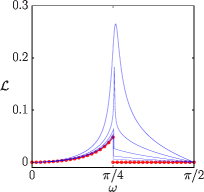
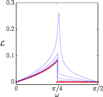
In Ref. Wichterich et al., 2010, Wichterich et al. have shown that once the Hamiltonian is written as a three-boson Hamiltonian, that is (19) with $p=3$, the logarithmic negativity is given by

$$\mathcal{L}=-\frac{1}{2}\ln\left[1+g-\sqrt{g^{2}+4\tau_{1}\tau_{3}(\alpha+1/\alpha-2)}\right],$$ (29)

with

$$g=\left[\tau_{1}+\tau_{3}-(\tau_{1}-\tau_{3})^{2}\right](\alpha+1/\alpha-2)/2,$$ (30)

where $\alpha$ is given in Eq. (22). This result, which is valid in the thermodynamical limit, is plotted in Fig. 7. One can furthermore see in this figure that the finite-size data from exact diagonalizations converge to the value (30) when the system size $N$ grows. In addition, all that was said for the behavior of the concurrence of the various models under investigation holds again here for the logarithmic negativity.

IV Conclusion

The concurrence, the entanglement entropy, and the logarithmic negativity, although different entanglement measures, show similar features when used to characterize the quantum phase transitions of the class of collective models we have introduced in this paper. However, when the transition is of first-order nature but accompanied by a collapse of levels on the ground state [see model $(2,2)$], as is usually characteristic of second-order transitions, the entanglement of the ground state does not show any discontinuity at the transition, but behaves exactly as in a usual second-order transition. In such a situation, one may wonder whether other “intrinsic measures” would be more sensitive to this discontinuous transition. One may think about studying the fidelity that has already been analyzed for the (2,1) (Lipkin-Meshkov-Glick) model at zero Kwok et al. (2008); Ma et al. (2008, 2009); Gu (2010) and at finite temperature Quan and Cucchietti (2009); Scherer et al. (2009) or to the geometric entanglement, which is also known for the (2,1) case Orús et al. (2008). We have computed these quantities for the (2,2) model and found that their behavior is similar in the (2,1) and the (2,2) cases although, as already underlined, finite-size scalings are different. We wish to underline that it this not an isolated case since, for all $(m,m)$ with $m\geqslant 2$, one has a first-order transition and the symmetry of the Hamiltonian under the exchange $(x\leftrightarrow z)$ implies that entanglement measures must be continuous. However, as can be checked from the exact formulas given in this paper, there is no entanglement for $(m,n)$ models when $m\geqslant n\geqslant 3$. Thus, from this perpspective the $(2,2)$ model is a bit singular.

To conclude, let us emphasize that we focused here on the ground-state entanglement. Nevertheless, it would be worth considering the full spectrum of these models to investigate finite-temperature entanglement, which may unveil interesting properties Canosa et al. (2007); Matera et al. (2008). This is beyond the scope of this paper but it will be the topic of a forthcoming publication J. Wilms et al. .

Appendix A Diagonalization of the two-mode Hamiltonian (19)

To compute the entanglement entropy, one needs to diagonalize the Hamiltonian (19) for $p=2$. This is done by performing the following Bogoliubov transformation :

$$a_{1} = \big{[}\cosh(\Theta/2)b_{1}+\sinh(\Theta/2)b_{1}^{\dagger}\big{]}\sqrt{\tau_{1}}+b_{2}\sqrt{\tau_{2}},\qquad$$ (31)

$$a_{2} = \big{[}\cosh(\Theta/2)b_{1}+\sinh(\Theta/2)b_{1}^{\dagger}\big{]}\sqrt{\tau_{2}}-b_{2}\sqrt{\tau_{1}},\qquad$$ (32)

where $\tanh\Theta=\varepsilon=-2\gamma/\delta$. New bosonic operators mutually commutes and satisfy $\left[b_{1},b_{1}^{\dagger}\right]=\left[b_{2},b_{2}^{\dagger}\right]=1$.

Inserting these relations in Eq. (19) for $p=2$, one gets :

$$H=Ne_{0}+\gamma+\frac{\delta}{2}\left(\sqrt{1-\varepsilon^{2}}-1\right)+\Delta_{1}b_{1}^{\dagger}b_{1}+\Delta_{2}b_{2}^{\dagger}b_{2},\\$$ (33)

where $\Delta_{1}=\delta\sqrt{1-\varepsilon^{2}}$ and $\Delta_{2}=\delta$.

References

- Amico et al. (2008) L. Amico, R. Fazio, A. Osterloh, and V. Vedral, Rev. Mod. Phys. 80, 517 (2008).
- Osborne and Nielsen (2002) T. J. Osborne and M. A. Nielsen, Phys. Rev. A 66, 032110 (2002).
- Osterloh et al. (2002) A. Osterloh, L. Amico, G. Falci, and R. Fazio, Nature (London) 416, 608 (2002).
- Vidal et al. (2003) G. Vidal, J. I. Latorre, E. Rico, and A. Kitaev, Phys. Rev. Lett. 90, 227902 (2003).
- Lipkin et al. (1965) H. J. Lipkin, N. Meshkov, and A. J. Glick, Nucl. Phys. 62, 188 (1965).
- Meshkov et al. (1965) N. Meshkov, A. J. Glick, and H. J. Lipkin, Nucl. Phys. 62, 199 (1965).
- Glick et al. (1965) A. J. Glick, H. J. Lipkin, and N. Meshkov, Nucl. Phys. 62, 211 (1965).
- Vidal et al. (2004a) J. Vidal, G. Palacios, and R. Mosseri, Phys. Rev. A 69, 022107 (2004a).
- Vidal et al. (2004b) J. Vidal, R. Mosseri, and J. Dukelsky, Phys. Rev. A 69, 054101 (2004b).
- Vidal et al. (2004c) J. Vidal, G. Palacios, and C. Aslangul, Phys. Rev. A 70, 062304 (2004c).
- Dusuel and Vidal (2004) S. Dusuel and J. Vidal, Phys. Rev. Lett. 93, 237204 (2004).
- Latorre et al. (2005) J. I. Latorre, R. Orús, E. Rico, and J. Vidal, Phys. Rev. A 71, 064101 (2005).
- Dusuel and Vidal (2005) S. Dusuel and J. Vidal, Phys. Rev. B 71, 224420 (2005).
- Unanyan et al. (2005) R. G. Unanyan, C. Ionescu, and M. Fleischhauer, Phys. Rev. A 72, 022326 (2005).
- Barthel et al. (2006) T. Barthel, S. Dusuel, and J. Vidal, Phys. Rev. Lett. 97, 220402 (2006).
- Vidal (2006) J. Vidal, Phys. Rev. A 73, 062318 (2006).
- Vidal et al. (2007) J. Vidal, S. Dusuel, and T. Barthel, J. Stat. Mech.: Theory Exp. P01015 (2007).
- Morrison and Parkins (2008) S. Morrison and A. S. Parkins, Phys. Rev. A 77, 043810 (2008).
- Cui (2008) H. T. Cui, Phys. Rev. A 77, 052105 (2008).
- Orús et al. (2008) R. Orús, S. Dusuel, and J. Vidal, Phys. Rev. Lett. 101, 025701 (2008).
- Caneva et al. (2008) T. Caneva, R. Fazio, and G. E. Santoro, Phys. Rev. B 78, 104426 (2008).
- Ma et al. (2009) J. Ma, X. Wang, and S.-J. Gu, Phys. Rev. E 80, 021124 (2009).
- Wichterich et al. (2010) H. Wichterich, J. Vidal, and S. Bose, Phys. Rev. A 81, 032311 (2010).
- Wootters (1998) W. K. Wootters, Phys. Rev. Lett. 80, 2245 (1998).
- Vidal and Werner (2002) G. Vidal and R. F. Werner, Phys. Rev. A 65, 032314 (2002).
- Kugel and Khomskii (1982) K. I. Kugel and D. I. Khomskii, Sov. Phys. Usp. 25, 231 (1982).
- Xu and Moore (2004) C. Xu and J. E. Moore, Phys. Rev. Lett. 93, 047003 (2004).
- Xu and Moore (2005) C. Xu and J. E. Moore, Nucl. Phys. B 716, 487 (2005).
- Nussinov and Fradkin (2005) Z. Nussinov and E. Fradkin, Phys. Rev. B 71, 195120 (2005).
- Maritan et al. (1984) A. Maritan, A. Stella, and C. Vanderzande, Phys. Rev. B 29, 519 (1984).
- Ribeiro et al. (2007) P. Ribeiro, J. Vidal, and R. Mosseri, Phys. Rev. Lett. 99, 050402 (2007).
- Ribeiro et al. (2008) P. Ribeiro, J. Vidal, and R. Mosseri, Phys. Rev. E 78, 021106 (2008).
- Pan and Draayer (1999) F. Pan and J. P. Draayer, Phys. Lett. B 451, 1 (1999).
- Links et al. (2003) J. Links, H.-Q. Zhou, R. H. McKenzie, and M. D. Gould, J. Phys. A 36, R63 (2003).
- Ortiz et al. (2005) G. Ortiz, R. Somma, J. Dukelsky, and S. Rombouts, Nucl. Phys. B 707, 421 (2005).
- Botet and Jullien (1983) R. Botet and R. Jullien, Phys. Rev. B 28, 3955 (1983).
- Holstein and Primakoff (1940) T. Holstein and H. Primakoff, Phys. Rev. 58, 1098 (1940).
- Wang and Mølmer (2002) X. Wang and K. Mølmer, Eur. Phys. J. D 18, 385 (2002).
- Kwok et al. (2008) H.-M. Kwok, W.-Q. Ning, S.-J. Gu, and H.-Q. Lin, Phys. Rev. E 78, 032103 (2008).
- Ma et al. (2008) J. Ma, L. Xu, H.-N. Xiong, and X. Wang, Phys. Rev. E 78, 051126 (2008).
- Gu (2010) S.-J. Gu, Int. J. Mod. Phys. B 24, 4371 (2010).
- Quan and Cucchietti (2009) H. T. Quan and F. M. Cucchietti, Phys. Rev. E 79, 031101 (2009).
- Scherer et al. (2009) D. D. Scherer, C. A. Müller, and M. Kastner, J. Phys. A 42, 465304 (2009).
- Canosa et al. (2007) N. Canosa, J. M. Matera, and R. Rossignoli, Phys. Rev. A 76, 022310 (2007).
- Matera et al. (2008) J. M. Matera, R. Rossignoli, and N. Canosa, Phys. Rev. A 78, 012316 (2008).
- (46) J. Wilms et al., in preparation.