Classification under Data Contamination with Application to Remote Sensing Image Mis-registration

Abstract

This work is motivated by the problem of image mis-registration in remote sensing and we are interested in determining the resulting loss in the accuracy of pattern classification. A statistical formulation is given where we propose to use data contamination to model the phenomenon of image mis-registration. This model is widely applicable to many other types of errors as well, for example, measurement errors and gross errors etc. The impact of data contamination on classification is studied under a statistical learning theoretical framework. A closed-form asymptotic bound is established for the resulting loss in classification accuracy, which is less than $\epsilon/(1-\epsilon)$ for data contamination of an amount of $\epsilon$. Our bound is sharper than similar bounds in the domain adaptation literature and, unlike such bounds, it applies to classifiers with an infinite VC dimension. Extensive simulations have been conducted on both synthetic and real datasets under various types of data contaminations, including label flipping, feature swapping and the replacement of feature values with data generated from a random source such as a Gaussian or Cauchy distribution. Our simulation results show that the bound we derive is fairly tight.

1 Introduction

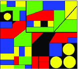
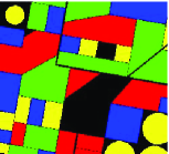
A motivating example of this work is the problem of image mis-registration which occurs almost ubiquitously in remote sensing. Image mis-registration refers to the phenomenon where the image of interest is mapped or aligned to a wrong position. This is usually caused by errors in the image or data acquisition device or the inaccuracy of the underlying mapping algorithms which try to map data collected at different scales, at different times, or taken from different angles. Figure 1 below illustrates an instance of image mis-registration where the image is tilted and then shifted by a small amount.

Figure 1: The original (left) and the mis-registered (right) remote sensing images for a cropland. Each color corresponds to one land class.

The problem of image registration is of primary importance in remote sensing land monitoring applications which typically require the use of a number of images acquired at different times or time sequence data that can characterize seasonal changes or multi-annual similarities (Defries and Townshend, 1999 [13]; Liu et al., 2006 [27]). This demands image registration and can affect such applications as image classification, change detection, ecological/climatological/hydrological modeling (Justice et al., 1998 [26]; Gong and Xu, 2003 [21]) etc. Because image registration can never be perfectly made, a mis-registration error is inevitable. It has been suggested that mis-registration errors that are less than 0.5 pixels are acceptable in subsequent analysis (Gong et al., 1992 [20]; Townshend et al. 1992 [36]; Jensen, 2004 [25]). However, this is rarely achievable and it is thus important to assess the impact of image mis-registration.

Of a similar nature are errors due to rounding or the inaccuracy of the measuring instruments. Besides, interference from electromagnetic waves, clouds or other unfavorable weather conditions can all cause errors to the remote sensing images. Additionally, various types of human errors often factor in where a small amount of arbitrary error maybe thrown in anywhere in the data or any part of the data can be missing. Errors of this type are often called gross errors, and are estimated to occur in about $0.1\%$ to $10\%$ of the data [22]. This estimation of the amount of errors will form the basis for our choice on the amount of data contamination in our simulation.

We call errors discussed above broadly as data contamination. Data contamination can cause a disastrous effect to the data quality and may fundamentally impact subsequent analysis and inference. It is thus of significant practical importance to answer the question: How much does data contamination impact our analysis (classification)? Do current algorithms (classifiers) continue to work or how much do we lose in accuracy if a remote sensing image is mis-registered or the underlying data are contaminated? The goal of the present work aims to shed lights on these questions. To gain insights into the nature of data contamination, in particular the phenomenon of image mis-registration, it is highly desired to approach the problem with a formal model and to give some theoretical characterization. This forms the primary motivation of the present work. Our focus will be on classification.

Assume the data of interest are drawn i.i.d. from some probability distribution $G$ defined on $\mathbb{R}^{p}$. By treating errors as contaminations to the probability distribution $G$, we arrive at the following statistical model for data contamination

$$\tilde{G}=(1-\epsilon)G+\epsilon{H}$$ (1)

where $\tilde{G}$ is the distribution of the data after contamination and $H$ is an arbitrary distribution. Model (1) is quite general, clearly it captures various types of data contaminations we have discussed (not the additive noise though). Note that, in the setting of classification, $G$ is the joint distribution of the attributes and the label, thus a contamination under model (1) can mean that to the attributes, or the label, or both. The $\epsilon$ in (1) can be thought of as the proportion of data (e.g., image pixels) that are “contaminated”, e.g., being flipped in label or altered with data generated under a different distribution $H$.

It is known that the effect of image mis-registration is determined by resolution, scene structure and amount of registration error (e.g., 0.5 pixels or 1 pixel, or 1.5 pixels on RMS error). In model (1), we choose to use the proportion of pixels that are “contaminated” as a measure of the extent of image mis-registration. This is to capture the essence of image mis-registration and to uncover the relationship between the amount of mis-registration and the resulting loss in classification accuracy. This is different from the usual practice in the remote sensing community where the image mis-registration is quantified in term of a shift of a certain number of pixels. Since given the same amount of shift, the impact on classification is highly scene-dependent, e.g., the impact would be drastically different for a large land consisting mainly of forests and a small land parcel formed by corn fields and rice fields, it would then hardly be possible to establish a generic relationship between the amount of mis-registration and the resulting loss on the classification accuracy.

Our contributions are as follows. We propose a statistical model for the phenomenon of image mis-registration. This data contamination model captures a wide range of errors such as label flipping, measurement errors, rounding errors and accidental human errors which occur almost ubiquitously in real applications. We study classification under data contamination in the statistical learning framework. A bound is obtained on the loss of classification accuracy (term this as the data contamination bound) due to data contamination (to the training data) in terms of its amount. This bound allows one to give a conservative assessment on if a class of classification algorithms, i.e., those which are universally consistent, continue to work under data contamination.

The rest of the paper is organized as follows. In Section 2, we formulate the problem of classification under data contamination and obtain a bound on the loss in classification accuracy in terms of the amount of data contamination. This is followed by a discussion of related work in statistics, remote sensing and machine learning in Section 3, and in particular we compare various aspects of our bound with the finite sample type of bounds established in the recently emerging area–domain adaptation. In Section 4, we conduct extensive simulations on the impact of data contamination to classification performance of SVM for a number of synthetic and real datasets under various types of data contaminations. In Section 4.5, we briefly discuss heuristics to estimate the amount of data contamination for the case of image mis-registration. Finally we conclude in Section 5. In this section, we also collect results from the literature on the impact of classification performance by AdaBoost due to label flipping; additionally, we give insight on using data contamination as a model to understand co-training, which is particularly useful in situations where training data are scarce.

2 Classification under data contamination

Classification is an important problem in pattern recognition. However, as discussed in Section 1, especially in the context of land-cover, land-use mapping, crop yield estimation and many other important applications in remote sensing, the classification result may be affected by data contamination. In this section, we will study classification under data contamination with model (1) and derive a bound on the resulting loss in classification accuracy. We start by an introduction of the statistical learning framework for classification [15].

2.1 Classification in the statistical learning framework

In statistical learning, a classification rule (or classifier) is defined by a map: $\mathcal{X}\rightarrow\mathcal{Y}$ where $\mathcal{X}$ is the sample space for observations and $\mathcal{Y}$ is a finite set of labels. For simplicity, we consider throughout a two-class problem where $\mathcal{Y}=\{0,1\}$.

Associated with each classifier, there is a performance measure called loss function, denoted by $l(f,X,Y)$. The loss function that is of special interest is the 0-1 loss, defined as

$$l(f,X,Y)=\left\{\begin{array}[]{ll}0&\mbox{if}~{}I_{\{f(X)>0\}}=Y\\ 1&\mbox{otherwise}\end{array}\right.$$ (2)

where $f$ is a decision function and $I_{\{.\}}$ is the indicator function. Here we call a function $f$ a decision function if a decision rule can be written as $I_{\{f>0\}}$.

Definition. Let $\mathbb{P}$ be the joint probability distribution of $X$ and $Y$. Then the risk associated with a decision function $f$ is defined as

$$R_{\mathbb{P}}(f) = \mathbb{E}_{\mathbb{P}}l(f,X,Y)=\mathbb{P}(Y\neq I_{\{f(X)>0\}}).$$ (3)

Similarly, the empirical risk for a decision function $f$, on a training sample $(X_{1},Y_{1}),...,(X_{n},Y_{n})$, can be obtained by replacing $\mathbb{P}$ in the above with its empirical distribution $\hat{\mathbb{P}}_{n}$.

Fix a probability distribution $\mathbb{P}$ and a function class $\mathcal{G}$, the goal of classification is to find a decision rule $f^{*}_{\mathcal{G}}\in\mathcal{G}$ that minimizes $R_{\mathbb{P}}(f)$, i.e.,

$$f^{*}_{\mathcal{G}}=\arg\min_{f\in\mathcal{G}}R_{\mathbb{P}}(f).$$ (4)

The rule learned from the training sample $(X_{1},Y_{1}),...,(X_{n},Y_{n})$, denoted by $f_{n}$, can be defined similarly by substitution of $\mathbb{P}$ with $\hat{\mathbb{P}}_{n}$ in (4).

Definition. Fix a probability distribution $\mathbb{P}$. The function that achieves the minimum risk, among all possible decision rules, is called the Bayes rule. The corresponding risk is called the Bayes risk and is denoted by $R_{\mathbb{P}}^{*}$.

For the 0-1 loss as defined in (2) and a fixed probability distribution, the Bayes rule is given by

$$\beta(x)=I_{\{\eta(x)>0\}}$$

where

$$\eta(x)=\mathbb{P}(Y=1~{}|~{}X=x)-0.5$$

is called the Bayes decision function.

Definition. A classification algorithm is universally consistent if, for all distributions $\mathbb{P}$,

$$R_{\mathbb{P}}(f_{n})\rightarrow_{a.s.}R_{\mathbb{P}}^{*}$$

as $n\rightarrow\infty$ where a.s. stands for almost surely.

Notation. To simplify notation, we adopt the following convention. Denote $R\triangleq R_{G}$ and $\tilde{R}\triangleq R_{\tilde{G}}$. Also we use $\tilde{}$ to indicate a quantity associated with the contaminated distribution $\tilde{G}$. In particular, $f_{n}$ and $\tilde{f}_{n}$ are the classifiers learned from a training sample of size $n$ from $G$ and $\tilde{G}$, respectively; and $\eta$, $\tilde{\eta}$ and $\eta^{H}$ are the Bayes decision function under $G$, $\tilde{G}$ and $H$, respectively.

2.2 A bound on the loss of classification accuracy

In the standard setting of statistical learning theory, one is interested in the consistency of a classifier, $f_{n}$, obtained via empirical risk minimization, that is,

$$R(f_{n})\longrightarrow R^{*}$$

as $n\rightarrow\infty$. In such a case, the classifiers $f_{n}$ are trained and tested with data generated from the same probability distribution $G$.

In the present work, we consider a different setting where the probability distribution, $\tilde{G}$, of the training sample differs from that of the test sample, $G$. Of course if $G$ and $\tilde{G}$ are “totally” different, then there is no hope of learning. We thus make the assumption that $G$ and $\tilde{G}$ differ by a small amount in the sense of a “small” $\epsilon$ under model (1). Clearly the rule learned from a training sample under $\tilde{G}$ will be different from that under $G$. Since the test sample is from $G$, classifier trained under $\tilde{G}$ would typically have a larger classification error. One important question is, how much additional classification error will be introduced if the classifier is trained on a sample from $\tilde{G}$ (instead of $G$) when testing on a sample generated from $G$.

Really we wish to know how much $R(\tilde{f}_{n})$ is different from $R(f_{n})$ as $n\rightarrow\infty$ for $\epsilon$ small. As we do not have access to data from $G$, a natural proxy for $R(f_{n})$ is $R^{*}$ since $R(f_{n})\rightarrow R^{*}$ as $n\rightarrow\infty$ for consistent classifiers $f_{n}$. We start by the following risk decomposition

$$R(\tilde{f}_{n})-R^{*} = R(\tilde{f}_{n})-R(\tilde{\eta})+R(\tilde{\eta})-R^{*}.$$ (5)

The $R(\tilde{\eta})-R^{*}$ term in (5) can be bounded by a term that depends only on the amount of contamination, $\epsilon$, under some weak assumptions. This is stated as Theorem 1. The term $R(\tilde{f}_{n})-R(\tilde{\eta})$ can be shown to vanish as the training sample size increases if the underlying classifier is universally consistent. This is stated as Theorem 2. Note that here the convergence rate may be different for different types of classifiers.

Theorem 1.

If $g(x)$, the probability density function of $G$, exists, then for data contamination with any distribution $H$,

$$R(\tilde{\eta})-R^{*} \leq \frac{\epsilon}{1-\epsilon},$$

where the equality holds if and only if the followings are true

• $$\epsilon=\frac{0.5-R^{*}}{1-R^{*}},~{}h(x)=\frac{|\eta(x)|g(x)}{1-2R^{*}},~{}\mbox{and}$$

• $P_{H}(Y=1|X=x)=1$ when $\eta(x)<0$, and 0 otherwise.

Remark.

1. The bound as stated in Theorem 1 is sharp as it is achievable under a special case as noted in the statement of the theorem.

2. A related data contamination model is as follows.

   $$d\tilde{G}(x)=[1-\epsilon(x)]dG(x)+\epsilon(x)dH(x)$$ (6)

   such that $0\leq\epsilon(x)\leq\epsilon<1$ for some positive constant $\epsilon$ where $G,H,\tilde{G}$ are probability distribution functions. Model (6) allows the amount of data contamination to be data dependent as long as the amount is uniformly smaller than a constant. Similar result as Theorem 1 can be obtained.

To prepare for the proof of Theorem 1, we have the following lemma.

Lemma 1.

Let $f$ be a decision function. Further assume $\mathbb{P}(f(X)=0)=0$. Then

$$R(f) = 0.5-\mathbb{E}\left[\eta(X).\mbox{sign}\left(f(X)\right)\right]$$

where $sign(x)=1~{}\mbox{if}~{}x>0~{}\mbox{and}~{}-1~{}\mbox{otherwise}$.

Proof.

Note that we can write

$$R(f)=\mathbb{E}_{G}\left|Y-I_{\{f(X)>0\}}\right|.$$

Thus

$$R(f) = \mathbb{E}\left[Y.I_{\{f(X)<0\}}\right]+\mathbb{E}\left[(1-Y).I_{\{f(X)>0\}}\right]$$

$$= 0.5+\mathbb{E}\left[(Y-0.5).I_{\{f(X)<0\}}\right]+\mathbb{E}\left[(0.5-Y).I_{\{f(X)>0\}}\right]$$

$$= 0.5-\mathbb{E}\left[\eta(X).\mbox{sign}\left(f(X)\right)\right].$$

∎

The posterior probability $\tilde{\eta}(x)+0.5$ under the contaminated distribution $\tilde{G}$ can be written as

$$\tilde{\eta}(x)+0.5=[1-\alpha_{\epsilon}(x)](\eta(x)+0.5)+\alpha_{\epsilon}(x)(\eta^{H}(x)+0.5)$$

where

$$\alpha_{\epsilon}(x) = \epsilon h(x)[(1-\epsilon)g(x)+\epsilon h(x)]^{-1}.$$

Here $g$ and $h$ are the continuous density or discrete probability functions corresponding to $G$ and $H$, respectively. Then

$$\tilde{\eta} = (1-\alpha_{\epsilon})\eta+\alpha_{\epsilon}\eta^{H}.$$

Proof of Theorem 1.

By Lemma 1, we have

$$R(\tilde{\eta})-R^{*} = \mathbb{E}\left[\eta(sign(\eta)-sign(\tilde{\eta}))\right]=2\mathbb{E}\left[|\eta|.I_{\{\eta\tilde{\eta}<0\}}\right].$$

Next notice that, if

$$\eta\tilde{\eta} = \alpha_{\epsilon}\eta^{2}\left[\frac{(1-\alpha_{\epsilon})}{\alpha_{\epsilon}}+\frac{2\eta^{H}}{2\eta}\right]<0,$$

then this implies

$$2|\eta| \leq \frac{\alpha_{\epsilon}}{(1-\alpha_{\epsilon})}=\frac{\epsilon}{1-\epsilon}\frac{h(x)}{g(x)}.$$

Hence,

$$R(\tilde{\eta})-R^{*} \leq 2\mathbb{E}\left[|\eta|.I_{\left\{2|\eta|\leq\frac{\epsilon}{1-\epsilon}\frac{h(X)}{g(X)}\right\}}\right]$$ (7)

$$\leq \frac{\epsilon}{1-\epsilon}\mathbb{E}\frac{h(X)}{g(X)}$$

$$= \frac{\epsilon}{1-\epsilon}.$$

The equality in (7) holds if and only if $\eta^{H}=-\frac{1}{2}$, or, $P_{H}(Y=1|X=x)=1$ when $\eta(x)<0$, and 0 otherwise, i. e. for the same observation $X=x$, the worst rule under $H$ assigns a completely oppositive class membership w.r.t. that under $G$. Further, the equality in (2.2) holds if and only if

$$2|\eta(x)|=\frac{\epsilon}{1-\epsilon}\frac{h(x)}{g(x)},$$

which implies

$$2\mathbb{E}|\eta| = \frac{\epsilon}{1-\epsilon}$$

since $\int h(x)dx=1$. Thus,

$$\epsilon=\frac{2\mathbb{E}|\eta|}{1+2\mathbb{E}|\eta|}=\frac{0.5-R^{*}}{1-R^{*}}$$

by Lemma 1. This concludes the proof. ∎

Theorem 2.

Suppose a classification algorithm is universally consistent. Then, under data contamination model (1), we have

$$R(\tilde{f}_{n})\rightarrow R(\tilde{\eta})$$

as $n\rightarrow\infty$.

The proof of Theorem 2 relies on the following lemma.

Lemma 2.

Assume $\mathbb{P}\left(\eta(X)=0\right)=0$. If $R(f_{n})\rightarrow R^{*}$, then the decision induced by $f_{n}$ converges to the Bayes rule in probability as $n\rightarrow\infty$.

Remark. Theorem 2 of Bartlett and Tewari [3] implies that the decision rule given by SVM converges to the Bayes rule. Lemma 2 is more general in that it applies to all consistent rules.

Proof.

Without loss of generality, assume the decision function $f_{n}$ is already centered, i.e., the corresponding decision rule can be written as $I_{\{f_{n}>0\}}$. From Lemma 1, we have

$$R(f_{n})=0.5-\mathbb{E}\left(\eta(X)*\mbox{sign}(f_{n}(X))\right).$$

Let

$$\xi_{n}(x)=|\mbox{sign}(\eta(x))-\mbox{sign}(f_{n}(x))|,$$

then $\xi_{n}(x)$ takes two values $\{0,2\}$. We have

$$R(f_{n})-R^{*}$$

$$= \mathbb{E}(\eta(X))\left[\mbox{sign}(\eta(x))-\mbox{sign}(f_{n}(x))\right]$$

$$= \mathbb{E}|\eta_{m}(X)|.\xi_{n}(X).$$

Thus, $\mathbb{P}(\xi_{n}(X)=2)\rightarrow 0$ by assumption $R(f_{n})\rightarrow R^{*}$ as $n\rightarrow\infty$. That is, $I_{\{f_{n}(X)>0\}}$ converges to $I_{\{\eta(X)>0\}}$ in probability as $n\rightarrow\infty$. ∎

Proof of Theorem 2.

By universal consistency and Lemma 2, we have

$$\int I_{\left\{\mbox{sign}(\tilde{f}_{n}(X))\neq\mbox{sign}(\tilde{\eta}(X))\right\}}d\tilde{G}(x)\rightarrow 0.$$

Thus

$$\int I_{\left\{\mbox{sign}(\tilde{f}_{n})\neq\mbox{sign}(\tilde{\eta})\right\}}dG\rightarrow 0,$$

implying that, as $n\rightarrow\infty$,

$$R(\tilde{f}_{n})\rightarrow R(\tilde{\eta}).$$

∎

By risk decomposition (5) as well as Theorem 1 and Theorem 2, we arrive at a sharp asymptotic data contamination bound as

$$\frac{\epsilon}{1-\epsilon}+O\left(c(n)\right).$$ (9)

where $c(n)=R(\tilde{f}_{n})-R(\tilde{\eta})$ indicates the rate of convergence with $c(n)\rightarrow 0$ as $n\rightarrow\infty$.

Bound (9) implies that, when the amount of data contamination is “small”, i.e., $\epsilon\rightarrow 0$, we can make

$$|R(\tilde{f}_{n})-R^{*}|\rightarrow 0.$$

That is, as long as a classifier is consistent in the standard setting and the amount of contamination is small in the sense of a small $\epsilon$, this classifier suffers very little from data contamination. This explains why, empirically, classifiers such as SVM or others work well even when a small fraction of labels are randomly flipped.

Theorem 2 relies on the universal consistency of a classifier. Fortunately, several of the currently most popular classifiers are universally consistent, for example, SVM [33] and Adaboost with early stopping [4].

3 Related work

The study of data analysis and statistical inference under data contamination has been a long-standing research topic in statistics and machine learning. The earliest work can be traced back to at least a half century ago, see, for example, Tukey [37] for a survey on sampling from contaminated distribution. Extensive studies have been carried out since under the name of robust estimation ([24, 22]), measurement error model ([18, 9, 14]) etc. However, work along this line concerns primarily problems on regression or estimation.

Relevant literature in remote sensing, however, has been sparse. Swain el al [35] investigated the impact of image mis-registration to classification. However, this work is purely empirical and their results depend highly on the underlying scenes in the image; for example, even under the same amount of mis-registration, the impact would be considerably different on images formed primarily by large forest lands and those formed by many small patches of different land types such as corns and plants. Additionally, Townshend el al [36] considered the impact of image mis-registration to change detection. Xu et al [39] study parameter estimation for a simple linear model under measurement errors due to a mismatch of locations and scales.

Related machine learning literature is much richer. Such work can be broadly divided into two stages. The first stage, roughly before year 2005, mostly deals with data contamination in the form of label flipping and empirical study of its impact on the performance of various classifiers. This includes Dietterich [16] and Breiman [8] which evaluate the robustness of learning algorithms such as bagging, AdaBoost and Random Forests against label flipping. Other work includes ([30, 32, 41]) and references therein. The second or the current stage, which is closely related to the present work, deals with domain adaptation. Domain adaptation is a broader concept than data contamination in that it does not specify explicitly the nature of the difference between the source (or training) distribution and the target (or test) distribution as long as their difference is small whereas data contamination almost exclusively refers to model (1). There have been numerous papers published on domain adaptation, including applications, theory and methods, and it is beyond the scope of the present paper to give a detailed account here. Work that is closest to ours include ([5, 28]) (see also references therein). In particular, Ben-David et al [5] established the following bound.

Theorem 3 ([5]).

Let $\mathcal{H}$ be a hypothesis space of VC dimension $d$. If $\mathcal{U}_{S}$, $\mathcal{U}_{T}$ are unlabeled samples of size $m^{\prime}$ each, drawn from the source distribution $\mathcal{D}_{S}$ and the target distribution $\mathcal{D}_{T}$ respectively, then for any $\delta\in(0,1)$, with probability at least $1-\delta$ (over the choice of the samples), for every $h\in\mathcal{H}$, the difference between the error rates $\epsilon_{S}$ and $\epsilon_{T}$ satisfies

$$\epsilon_{T}(h)-\epsilon_{S}(h)$$

$$\leq \frac{1}{2}\hat{d}_{\mathcal{H}\Delta\mathcal{H}}(\mathcal{U}_{S},\mathcal{U}_{T})+4\sqrt{\frac{2d\log(2m^{\prime})+\log(2/\delta)}{m^{\prime}}}+\lambda$$

where $\lambda$ is defined by

$$\lambda=\arg\min_{h\in\mathcal{H}}[\epsilon_{S}(h)+\epsilon_{T}(h)]$$

with the subscripts $S,T$ indicating quantities related to the source and target, respectively.

The bound established in [28] is similar in nature which replaces the VC dimension in [5] with the Rademacher complexity [2]. However, there are important differences between the bound in Theorem 3 or that in [28] and ours (i.e., Theorem 1).

• The nature of bounds is different. The bounds in ([5, 28]) are finite sample learning generalization type of bounds while our bound is a large sample bound (i.e., asymptotic bound).

• The quality of the bounds is different. The bounds in [5] are union bounds that rely on the Vapnik-Chervonekis (VC) dimension [38], and are often quite loose ([28] uses the Rademacher complexity [2] but still quite loose). In contrast, our bound is a sharp bound asymptotically. Assume the underlying function class has a finite VC dimension and let $m^{\prime}\rightarrow\infty$, then the bound in Theorem 3 becomes $\epsilon+\lambda$, which is looser than our bound $\epsilon/(1-\epsilon)\approx\epsilon$ for small $\epsilon$. Since the $\lambda$ term depends on the difficulty of the underlying problem and generally does not vanish, in no way would the bounds in [5] imply ours.

  To better appreciate the difference in the quality of the bounds when the sample size increases, we will show an example where the data is generated by a two-component Gaussian mixture and contaminated by Cauchy data (See Section 4 for details on the Gaussian mixture and the Cauchy). Since it is not easy to directly compute $\lambda$, we replace it with its lower bound $\arg\min_{h\in\mathcal{H}}\epsilon_{S}(h)+\arg\min_{h\in\mathcal{H}}\epsilon_{T}(h)$, which are estimated as the error rates of SVM on the data when the training sample size is large. Figure 2 shows the asymptotic data contamination bounds of ours and that established in [5] for the amount of data contamination varying from $\{0.01,0.02,0.03,0.04,0.05,0.10\}$. One can see that here the Ben-David et al bound [5] is much looser than ours, and for this particular Gaussian mixture data, the Ben-David et al bound is not very informative as it quickly approaches $0.5$.

  

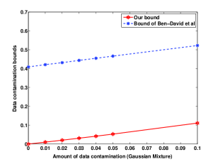
  Figure 2: Comparison of data contamination bound for Gaussian mixture data with $\epsilon\in\{0.01,0.02,0.03,0.04,0.05,0.10\}$.

• Whereas our bound applies only to universally consistent classifiers, the bound in [5] applies only to classifiers from a function class with a finite VC dimension. This is a limitation that cannot be overlooked. For example, the function class corresponding to the Gaussian kernel (see discussion after example 1.9 in [34] and the fact that the Gaussian kernel is a universal kernel), or the polynomial kernel (if no upper bound is imposed on the degree of polynomials), or the one nearest neighbor classifier, or the tree-based classifier (without regularization) all have an infinite VC dimension. Consequently, the bound in ([5]) excludes some of the best classifiers available today, including SVM with the Gaussian kernel, Boosting (or Bagging [7]) on tree-based classifiers etc while our bound clearly does not have such a restriction.

4 Experiments

Empirical studies are performed on three different types of datasets, $3$ synthetic datasets, $10$ UC Irvine datasets [1] and a simulated remote sensing image. For each dataset, four different types of data contaminations are applied to the training set and classification accuracy evaluated on the uncontaminated test set. SVM is used as the underlying classifier due to its universal consistency [33] and the availability of a widely used software implementation (libsvm [10]).

The five different types of data contaminations are as follows.

• Randomly flip the labels of a randomly selected subset of observations from a fixed class.

• Randomly flip the labels of a randomly selected subset of observations from all classes.

• Randomly select a subset of observations and replace the feature values of each with that of a randomly chosen observation (the labels are kept). Call this feature swapping.

• Replace a randomly selected subset of observations with Cauchy data with the labels kept.

• Replace a randomly selected subset of observations with Gaussian data with the labels kept.

Figure 3: Scatter plot of $1000$ observations generated i.i.d. from Gaussian $\mathcal{N}(\mu,\Sigma)$ with $\mu=(1,0)$ and $\Sigma=A^{t}A$ with entries of $A$ generated i.i.d. from $\mathcal{U}[0,1]$. Data from the two classes are represented as diamonds and solid circles, respectively.

Figure 4: Illustration of the effect of different types of data contamination. The original Gaussian data are displayed in Figure 3. The $4$ rows of plots correspond to $C_{1},C_{2},C_{g},C_{c}$, respectively and figures in the left and right columns are for data contamination at $5\%$ and $10\%$, respectively. Data from the two classes are represented as diamonds and solid circles, respectively.

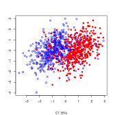
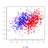
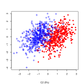
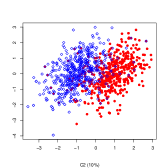
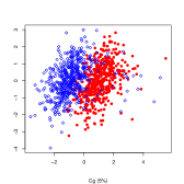
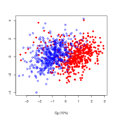
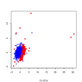
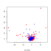
$C_{0},C_{1},...,C_{g}$ are used to simulate data contamination of different natures.

• $C_{1}$ and $C_{2}$ are expressly designed to simulate image mis-registration, which we believe capture important aspects of image mis-registration.

• $C_{c}$ and $C_{g}$ are used to simulate gross errors. $C_{g}$ is for errors with a Gaussian nature while $C_{c}$ is for errors with a heavy tail, that is, the error could be very large and this is to simulate accidental human error, for example, a shift in decimal place of a number.

• Additionally, we also attempt to simulate extremely large errors by scaling the centers of the Gaussian and Cauchy by a factor of $100$, that is, the centers are multiplied by $100$ coordinate-wisely. These are denoted by $C_{g100}$ and $C_{c100}$, respectively.

• $C_{0}$ is used to simulate a class of unfavorable situations where data contamination occurs in part of the data space. Such cases typically make classification more challenging. In contrast, other simulations are more or less average cases as the data contamination occurs uniformly across the whole data space.

For $C_{g}$, the replacement Gaussian data is generated i.i.d. from $\mathcal{N}(\mu,\Sigma)$ with $\mu$ and $\Sigma$ calculated empirically on the non-contaminated training set. For $C_{c}$, the Cauchy data is generated i.i.d. according to

$$Z/W,\quad\mbox{for}~{}Z\sim\mathcal{N}(\mu,\Sigma),~{}W\sim[\Gamma(0.5,2)]^{1/2}$$

with $Z$ and $W$ independent where $\Gamma(0.5,2)$ is a random variable generated from a Gamma distribution with parameters $0.5$ and $2$. For each run, $\mu$ is generated uniformly from the interval $[\min(X),\max(X)]$ and $\Sigma$ estimated empirically from the training set.

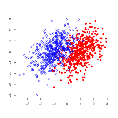
For an illustration of the effect of these different types of data contamination, see Figure 3 for the original data and Figure 4 for the data after contamination of different types.

4.1 Synthetic data

The three synthetic datasets used in our experiment are the Gaussian mixture data, the four-class and the nested-square data. The Gaussian mixture data are used to simulate cases with a linear decision boundary while the four-class and the nested-square datasets are for cases where the decision boundary is highly nonlinear and non-convex. For each of the $3$ datasets, we take $80\%$ for training and the rest for test. Then $100$ instances of data contamination are applied and loss in classification accuracy are averaged. This is repeated and results are averaged. The Gaussian kernel is used with SVM for all three synthetic datasets.

The Gaussian mixture data are generated according to the following

$$\Delta\mathcal{N}(\mu,\Sigma_{10\times 10})+(1-\Delta)\mathcal{N}(-\mu,\Sigma_{10\times 10})$$

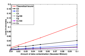
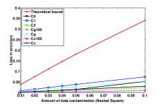
with $\mathbb{P}(\Delta=1)=\mathbb{P}(\Delta=0)=\frac{1}{2}$ and $\Sigma_{10\times 10}=A^{T}A$ for entries of $A$ generated i.i.d. uniform from $[0,1]$, with $\mu=(0.5,...,0.5)^{T}$. Data points with $\Delta=1$ are assigned label $1$ and those with $\Delta=0$ are assigned label $2$. The sample size for the training set and test set are $1000$ and $2000$, respectively. Loss in classification accuracy under data contamination of different types and at different amounts are shown in Figure 5. Note that here we are using only the first term in (9) as an estimate of the overall loss in classification accuracy while ignoring the second term, thus when the training sample size is not large enough, some adjustment (in the order of $O(c(n))$) might be required.

Figure 5: Empirical and theoretical data contamination bound for data generated from a Gaussian mixture with $\epsilon\in\{0.01,0.02,0.03,0.04,0.05,0.10\}$.

Figure 6: The four-class and nested-square data. Different colors correspond to points from different classes.

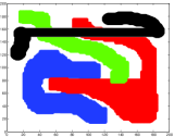
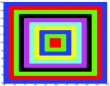
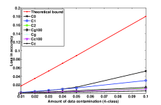
The four-class and nested-square datasets were originally used to demonstrate the superior performance of a class of projectable classifiers for data with a highly complex decision boundary [23]. Figure 6 is a plot of these two datasets and the data contamination bounds are shown in Figure 7. Note that the bound as established in (9) is for 2-class classification. When there are multiple classes, we can get a bound by repeatedly apply the the 2-class bound. Let the class distribution be denoted by $\{w_{1},...,w_{J}\}$ such that $w_{1}\geq...\geq w_{J}$. Then we get the following multi-class bound

$$\frac{\epsilon}{1-\epsilon}\left\{1+(w_{2}+...+w_{J})\alpha+...+(w_{\{J-1\}}+w_{J})\alpha^{J-2}\right\}$$

where $\alpha=1-\frac{\epsilon}{1-\epsilon}$ and $\epsilon$ is the mount of contamination. This is used as the theoretical bound in our simulations when there are more than two classes.

Figure 7: Empirical and theoretical data contamination bound for the 4-class and the nested-square datasets with $\epsilon\in\{0.01,0.02,0.03,0.04,0.05,0.10\}$.

4.2 UC Irvine datasets

A total of $10$ datasets are taken from the UC Irvine Machine Learning Repository [1] in our experiment. A summary of these datasets is provided in Table 1 and more details can be found from [1].

Table 1: Summary of the UC Irvine datasets used in our experiment.

	Training	Testing	Features	Classes
$imageSeg$	210	2100	19	7
$Vowel$	528	462	10	11
$Satellite~{}images$	4435	2000	36	6
$Glass$	214	–	10	6
$Vehicle$	946	–	18	4
$German~{}credit$	1000	–	24	2
$Yeast$	1484	–	8	10
$Wine~{}quality$	1599	–	11	6
$Musk$	6598	–	168	2
$Magic~{}gamma$	19020	–	10	2

Some data sets come with predetermined training and test sets, which includes the image segmentation, vowel and satellite image datasets. Otherwise we split the data into a training and test set. For small to medium sized datasets, i.e., Glass, Vehicle, German Credit, Yeast and Wine Quality (red wine), we take $80\%$ of the data for training and the rest for test. For large datasets, i.e., the Musk and Magic Gamma Telescope, $20\%$ and $10\%$, respectively, of the data are set aside for training and the rest for test. For each dataset, $100$ instances of data contamination are applied to the training set and the resulting data contamination bounds are averaged. This is repeated and results averaged.

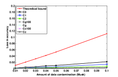
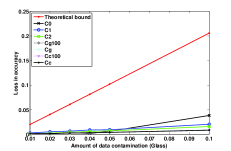
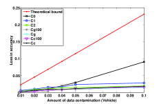
The Gaussian kernel is used for all except the image segmentation dataset where a polynomial kernel with degree $3$ is used. Tuning parameters for SVM are chosen so that the classification performance matches that reported in the literature (see, for example, references cited in the description of each dataset in [1]). Some datasets are linearly scaled to $[0,1]$ so as to speed up the painfully slow optimization of the SVM package; this includes the Musk, Magic Gamma, Satellite image, Vehicle, and the Wine quality dataset. The data contamination bounds by SVM on the UC Irvine datasets are plotted in Figure 8.

Figure 8: Empirical and theoretical data contamination bound for UC Irvine datasets (only $6$ of them are shown here so that they can be placed in the same page, the rest are similar) with $\epsilon\in\{0.01,0.02,0.03,0.04,0.05,0.10\}$.

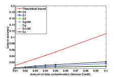
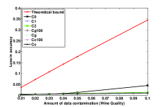
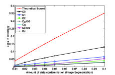
4.3 Remote sensing image

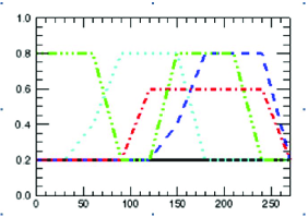
The remote sensing image used in the experiment is about a cropland with $5$ different land-use classes. The image size is $596$ pixel by $529$ pixel. The features of interest are taken from the annual vegetation index time series (see Figure 9) at an interval of $30$ days among which $10$ are used with each corresponding to one scene of image at a different time of the year. The vegetation index is an optical measure of vegetation canopy greenness and is closely related to the photosynthetic potential of plants. For each pixel, random noises, generated from Gaussian $\mathcal{N}(0,0.1^{2})$, are applied.

Figure 9: The annual vegetation index. The x-axis is the day of a year and different colors indicate different land classes.

To simulate the acquisition of remote sensing images, the following procedure is performed on each of the $10$ scenes of image.

1. Rotate all images clockwisely by $10$ degrees.

2. Re-sample each scene of image using a randomly generated offset from $\mathcal{N}(0,0.1^{2})$.

3. Remove the blank edges in all images that are caused by rotation and re-sampling.

In Step 2 of the above, offsets are generated from the standard Gaussian and a bilinear interpolation [19] is applied during re-sampling. As a result, $247$ pixel by $233$ pixel multi-temporal vegetation index images for the cropland of interest are generated.

To assess the impact of image mis-registration to the task of classification, two mis-registered images (corresponding to Case I and II in Table 2, respectively) are generated under different levels of mis-registration (roughly corresponding to $3\%$ and $4\%$ data contamination, respectively). The SVM classifier is trained on a sample from the original image and the mis-registered image, respectively, and then test on a sample taken from the original image. We use the data in a similar fashion as the 5-fold cross-validation, i.e., select $4$ folds for training and rest for testing. Table 2 reports the classification accuracy. We can see that, in both cases, the loss in classification accuracy is small and can be well bounded by our theoretical predication.

Table 2: Accuracy of SVM for the cropland remote sensing image under different amount of image mis-registration. Each of the first $5$ columns corresponds to one of the $5$ folds.

Fold	1	2	3	4	5	Average
$Original$	98.13	98.14	97.90	97.94	97.98	98.02
Case I	98.08	98.11	97.92	97.94	97.98	98.01
Case II	98.09	98.10	97.92	97.92	97.96	97.99

It is known that, for example by bootstrap, the effect of mis-registration on image classification varies with the relative size of the ground area corresponding to an image pixel (call this the pixel size) and the actual homogeneity (larger numbers correspond to more homogeneity) of an area. If the ratio of these two numbers is small, then the damage of mis-registration is small, otherwise it is large. Since we are using a crop field here and the corresponding pixel size is much smaller than that for the crop field, the effect of data contamination is small. If the pixel size is close to the actual object size, then mis-registration of half a pixel may cause more damages.

4.4 Some empirical results on Adaboost

So far SVM has been used as the underlying classifier in our experiment, other universally consistent classifiers such as Adaboost are applicable as well. Instead of repeating the experiment for AdaBoost, we collect results found in the literature [17, 16, 8] and summarize in Table 3. Note here we simply adopt the existing results and this corresponds to taking $\epsilon=0.05$ only.

Table 3: Error rates of Adaboost on some UC Irvine datasets where 90% of the data are used as the training set. Results are shown for the original data and when 5% of the class labels in the training set are randomly flipped (uniformly into an alternate class). Results are adopted from [8, 17, 16] and then converted.

	Original data	5% labels flipped	Difference
$Glass$	22.00%	22.35%	0.35%
$Breast~{}cancer$	3.20%	4.58%	1.38%
$Diabetes$	26.60%	28.41%	1.81%
$Sonar$	15.60%	17.96%	2.36%
$Ionsphere$	6.40%	8.17%	1.77%
$Soybean$	7.57%	9.61%	2.04%
$Ecoli$	14.80%	15.91%	1.11%
$Votes$	4.80%	7.14%	2.34%
$Liver$	30.70%	33.86%	3.16%

4.5 Estimating the amount of data contamination

Using data contamination bound (9), we can estimate the loss in accuracy for classifiers trained with contaminated data. The remaining question is to give a (rough) estimate of the amount of data contamination. This is a question we would like to leave to future work.

In the special case of image mis-registration, we propose two simple heuristics for estimating the amount of data contamination. Both are based on the heuristic that the image pixels affected by mis-registration are roughly those near the boundary between different land classes. Thus the proportion of boundary pixels serves as a good indication on the amount of data contamination. Here the underlying assumption is that the proportion of boundary pixels are roughly the same in the true and the mis-registered images.

One approach is based on sampling. A number, say $100$ to $200$, of pixels are randomly sampled from the image, we then count the proportion of pixels that fall on the boundary by visual inspection. Another estimate is based on the classification results by a classifier trained on the contaminated data. For each pixel, we determine if it is on the boundary by the following heuristic. For each pixel in the image, take a $3\times 3$ patch centering on it. If there are at least two pixels within the patch having a different class labels from the rest, then declare the pixel at the center of the patch to be on the boundary.

5 Conclusion and discussion

We formulate the problem of image mis-registration as data contamination and equip it with a statistical model. This model captures a very general class of errors, for instance, measurement errors and gross errors that can be formulated as label-flipping, feature-swapping, or feature replacement by any proper distributions. Under a statistical learning theoretical framework, we derive an asymptotic bound for the loss in classification accuracy due to data contamination. One nice feature about this bound is that, it is essentially distribution-free thus it applies to all different types of data. Extensive simulations on both synthetic and real datasets under various types of data contaminations show that the data contamination bound we derive is fairly tight. Compared to similar bounds in the domain adaptation literature, our bound is sharper and, unlike such bounds, our bound applies to classifiers with an infinite VC dimension.

As we have already discussed, our data contamination model can capture various types of errors such as image mis-registration, label noise and accidental human errors. Beyond that, we can also use data contamination as a useful device. We give here an example in the setting of co-training ([40, 6, 11]). Empirically, it has been shown that co-training can significantly boost the classification accuracy when the training sample size is extremely small, e.g., $12$ in [6] for web page classification and $6$ in [29] for newsgroup classification. Theoretical work have been carried out to understand the success of co-training (see, for instance, [6, 12]). We provide here a different perspective.

Figure 10: The benefit of co-training. $Err^{*}$ denotes the Bayes error rate.

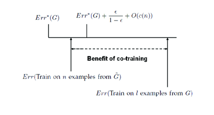
In co-training, starting from a small amount of labeled examples, the algorithm progressively enlarges the labeled set by transferring those examples which are originally unlabeled but are classified with high confidence by the classifier built from the labeled data available so far. This amounts to enlarging the labeled set with a small amount of label noise; the label noise here is small because those examples which are being transferred are classified with high confidence. Assume at certain point we have $n$ examples in the labeled set and assume $n$ is large, then, by our analysis (c.f. (9)), the additional classification error w.r.t. that resulting from a clean labeled set (of size $n$) is no more than $\epsilon/(1-\epsilon)+O(c(n))$ for $c(n)\rightarrow 0$ as $n$ grows. Thus,

$$Err(\mbox{Bayes classifier on $G$})$$

$$\leq Err(\mbox{Classifier learned on $n$ observations from $\tilde{G}$})$$

$$\leq Err(\mbox{Bayes classifier on $G$})+\frac{\epsilon}{1-\epsilon}+O\left(c(n)\right)$$

where $Err$ denotes the error rate. Here, we use $G$ and $\tilde{G}$ to denote the data with clean label and that containing labels assigned by the co-training algorithm, respectively. It is clear that the error rate achieved by co-training equals that by a classifier learned on $n$ observations from $\tilde{G}$. However, it is often the case that the error rate by a classifier learned on $l$ labeled examples from $G$ is typically much larger, i.e.,

$$Err(\mbox{Classifier learned on $l$ examples from $G$})$$ (10)

$$\gg Err(\mbox{Bayes classifier on $G$})+\frac{\epsilon}{1-\epsilon}+O\left(c(n)\right)$$

if $l$ is small, $\epsilon$ is small and $n$ is large. The gap between the two $Err$ terms in (10) is the potential “benefit” of co-training as illustrated in Figure 10. This explains why co-training may be feasible with a small amount of initial labeled examples. Since the gap in (10) shrinks as $l$ increases, this, on the other hand, explains why co-training may not help much when the initial labeled set is large.

A limitation of our data contamination model (1) is that, in modeling the phenomenon of image mis-registration with a data contamination model, i.i.d. contaminations are assumed. However, in practice the mis-registered image pixels may be correlated in some way. It is thus desirable to take this into account in the model, which we shall leave to future work. Note that we derive the data contamination bound under a general class of data distributions, it is desired to take advantage of knowledge on the underlying distribution to get a sharper bound. Note also that the focus of the present paper is the analysis and simulation on the impact of data contamination to classification accuracy, no new algorithm is proposed. We shall leave that to future work, interested readers can see, for example, [31] and references therein.

References

- [1] A. Asuncion and D. J. Newman. UCI Machine Learning Repository, Department of Information and Computer Science. http://www.ics.uci.edu/ mlearn/MLRepository.html, 2007.
- [2] P. L. Bartlett and S. Mendelson. Rademacher and gaussian complexities: Risk bounds and structural results. In COLT, pages 224–240, 2001.
- [3] P. L. Bartlett and A. Tewari. Sparseness vs estimating conditional probabilities: Some asymptotic results. Journal of Machine Learning Research, 8:775–790, 2007.
- [4] P. L. Bartlett and M. Traskin. Adaboost is consistent. Journal of Machine Learning Research, 8:2347–2368, 2007.
- [5] S. Ben-David, J. Blitzer, K. Crammer, A. Kulesza, F. Pereira, and J. Wortman Vaughan. A theory of learning from different domains. Machine Learning, 79:151–175, 2010.
- [6] A. Blum and T. Mitchell. Combining labeled and unlabeled data with co-training. In Proceedings of the eleventh annual conference on Computational learning theory, pages 92–100, 1998.
- [7] L. Breiman. Bagging predicators. Machine Learning, 24(2):123–140, 1996.
- [8] L. Breiman. Random Forests. Machine Learning, 45(1):5–32, 2001.
- [9] R. J. Carroll, A. Delaigle, and P. Hall. Nonparametric prediction in measurement error models. Journal of the American Statistical Association, 2009 (To appear).
- [10] C.-C. Chang and C.-J. Lin. LIBSVM: a library for support vector machines, 2001. Software available at http://www.csie.ntu.edu.tw/ cjlin/libsvm.
- [11] Michael Collins and Yoram Singer. Unsupervised models for named entity classification. In In Proceedings of the Joint SIGDAT Conference on Empirical Methods in Natural Language Processing and Very Large Corpora, pages 100–110, 1999.
- [12] S. Dasgupta, M.L. Littman, and D. McAllester. PAC generalization bounds for co-training. In Proceedings of Neural Information Processing Systems (NIPS), pages 375–382, 2001.
- [13] R. S. Defries and J. R. G. Townshend. Global land cover characterization from satellite data: from research to operational implementation? Global Ecology and Biogeography, 8(5):367–379, 1999.
- [14] A. Delaigle, J. Fan, and R. J. Carroll. A design-adaptive local polynomial estimator for the errors-in-variables problem. Journal of the American Statistical Association, 104:348–359, 2009.
- [15] L. Devroye, L. Györfi, and G. Lugosi. A Probabilistic Theory of Pattern Recognition (Stochastic Modelling and Applied Probability). Springer, 1996.
- [16] T. G. Dietterich. An experimental comparison of three methods for constructing ensembles of decision trees: Bagging, boosting and randomization. Machine Learning, 40(2):139–157, 1998.
- [17] Y. Freund and R. E. Schapire. Experiments with a new boosting algorithm. In Proceedings of the 13rd International Conference on Machine Learning (ICML), 1996.
- [18] W. A. Fuller. Measurement Error Models. John Wiley, 1987.
- [19] J. Gomes, L. Darsa, B. Costa, and L. Velho. Warping and Morphing of Graphical Objects. Morgan Kaufmann, 1998.
- [20] P. Gong, E. F. LeDrew, and J. R. Miller. Registration noise reduction in difference images for change detection. International Journal of Remote Sensing, 13(4):773–779, 1992.
- [21] P. Gong and B. Xu. Remote sensing of forests over time: change types, methods, and opportunities. In M. Woulder and S. E. Franklin, editors, Remote Sensing of Forest Environments: Concepts and Case Studies, pages 301–333. Kluwer Press, Amsterdam, Netherlands, 2003.
- [22] F. R. Hampel. The influence curve and its role in robust estimation. Journal of the American Statistical Association, 69(346):383–393, 1974.
- [23] T. K. Ho and E. M. Kleinberg. Building projectable classifiers of arbitrary complexity. In International Conference on Pattern Recognition, 1996.
- [24] P. J. Huber. Robust statistics: A review (The 1972 Wald Lecture). The Annals of Mathematical Statistics, 43(4):1041–1067, 1972.
- [25] J. R. Jensen. Introductory Digital Image Processing. Prentice Hall, 2004.
- [26] C. O. Justice, E. Vermote, J. R. G. Townshend, R. Defries, D. P. Roy, D. K. Hall, V. V. Salomonson, J. L. Privette, G. Riggs, A. Strahler, W. Lucht, R. B. Myneni, Y. Knyazikhin, S. W. Running, R. R. Nemani, Z. Wan, A. R. Huete, W. van Leeuwen, R. E. Wolfe, L. Giglio, J. Muller, P. Lewis, and M. J. Barnsley. The moderate resolution imaging spectroradiometer (MODIS): Land remote sensing for global change research. IEEE Transactions on Geoscience and Remote Sensing, 36(4):1228–1249, 1998.
- [27] D. Liu, M. Kelly, and P. Gong. A spatio-temporal approach to monitoring forest disease spread using multi-temporal high spatial resolution imagery. Remote Sensing of Environment, 101(2):167–180, 2006.
- [28] Y. Mansour, M. Mohri, and A. Rostamizadeh. Domain adaptation: Learning bounds and algorithms. In COLT, 2009.
- [29] K. Nigam. Understanding the behavior of co-training. In In Proceedings of KDD-2000 Workshop on Text Mining, 2000.
- [30] J. Quinlan. The effect of noise on concept learning. In R. S. Michalski, J. G. Carbonell, and T. M. Mitchell, editors, Machine Learning, an Artificial Intelligence Approach, Volume II, pages 149–166. Morgan Kaufmann, 1986.
- [31] P. K. Shivaswamy, C. Bhattacharyya, and A. J. Smola. Second order cone programming approaches for handling missing and uncertain data. Journal of Machine Learning Research, 7:1283–1314, 2006.
- [32] R. H. Sloan. Types of noise in data for concept learning. In The First Workshop on Computational Learning Theory, pages 91–96. Morgan Kaufmann, 1988.
- [33] I. Steinwart. Support vector machines are universally consistent. Journal of Complexity, 18:768–791, 2002.
- [34] I. Steinwart. Consistency of support vector machines and other regularized kernel machines. IEEE Transactions on Information Theory, 51:128–142, 2005.
- [35] P. H. Swain, V. C. Vanderbilt, and C. D. Jobusch. A quantitative applications-oriented evaluation of thematic mapper design specifications. IEEE Transactions on Geoscience and Remote Sensing, 20(3):370–377, 1982.
- [36] J. R. G. Townshend, C. O. Justice, C. Gurney, and J. McManus. The impact of mis-registration on change detection. IEEE Transactions on Geoscience and Remote Sensing, 30(5):1054–1060, 1992.
- [37] J. W. Tukey. A survey of sampling from contaminated distributions. In I. Olkin, editor, Contributions to Probability and Statistics, pages 448–485. Standford University Press, 1960.
- [38] V. N. Vapnik. Statistical Learning Theory. John Wiley, 1998.
- [39] Y. Xu, B. G. Dickson, H. M. Hampton, T. D. Sisk, J. A. Palumbo, and J. W. Prather. Effects of mismatches of scale and location between predictor and response variables on forest structure mapping. Photogrammetric Engineering & Remote Sensing, 75(3):313–322, 2009.
- [40] David Yarowsky. Unsupervised word sense disambiguation rivaling supervised methods. In in Proceedings of the 33rd Annual Meeting of the Association for Computational Linguistics, pages 189–196, 1995.
- [41] X. Zhu and X. Wu. Class noise vs. attribute noise: a quantitative study of their impacts. Artificial Intelligence Review, 22(3):177–210, 2004.