DIAS-STP-11-01

A manifestly MHV Lagrangian for $\mathcal{N}=4$ Yang–Mills

Sudarshan Ananth^†, Stefano Kovacs^∗ and Sarthak Parikh^†

^† Indian Institute of Science Education and Research

  Pune 411021, India

^∗ Dublin Institute for Advanced Studies

  10 Burlington Road, Dublin 4, Ireland

Abstract

We derive a manifestly MHV Lagrangian for the $\mathcal{N}=4$ supersymmetric Yang–Mills theory in light-cone superspace. This is achieved by constructing a canonical redefinition which maps the ${\mathcal{N}}=4$ superfield, $\phi$, and its conjugate, $\bar{\phi}$, to a new pair of superfields, $\chi$ and $\widetilde{\chi}$. In terms of these new superfields the ${\mathcal{N}}=4$ Lagrangian takes a (non-polynomial) manifestly MHV form, containing vertices involving two superfields of negative helicity and an arbitrary number of superfields of positive helicity. We also discuss constraints satisfied by the new superfields, which ensure that they describe the correct degrees of freedom in the ${\mathcal{N}}=4$ supermultiplet. We test our derivation by showing that an expansion of our superspace Lagrangian in component fields reproduces the correct gluon MHV vertices.

1 Introduction

The ${\mathcal{N}}=4$ supersymmetric Yang–Mills (SYM) theory has a number of remarkable properties, some of which have been known for a long time and others which have emerged more recently. The theory has maximal rigid supersymmetry and is an example of an interacting conformal field theory in four dimensions. It has been extensively studied – together with some of its deformations – for the special role it plays in the AdS/CFT correspondence [1, 2, 3]. The original formulation of the correspondence relates ${\mathcal{N}}=4$ SYM to type IIB string theory in an AdS${}_{5}\times S^{5}$ background and this remains the best understood and most thoroughly tested example of the duality. The ${\mathcal{N}}=4$ Yang–Mills theory also possesses a non-perturbative SL(2,$\mathbbm{Z}$) symmetry, known as S-duality, which generalises the electric-magnetic duality of Maxwell’s equations in the vacuum. This symmetry has recently been studied in connection with the so-called geometric Langlands program [4, 5, 6]. In another remarkable development, an integrable structure underlying the spectrum of scaling dimensions of ${\mathcal{N}}=4$ gauge-invariant composite operators has been discovered, see [7] and references therein for a recent comprehensive review. This finding is a further indication of the richness of the ${\mathcal{N}}=4$ theory. It is also the basis of powerful techniques developed for the calculation of quantum corrections to the scaling dimensions, which have allowed extremely accurate tests of the AdS/CFT duality [8].

In the past few years the study of scattering amplitudes in the ${\mathcal{N}}=4$ theory has attracted considerable interest. This is in spite of the fact that, as a conformally invariant non-Abelian gauge theory, ${\mathcal{N}}=4$ SYM does not possess well defined asymptotic states, making the physical relevance of scattering amplitudes somewhat dubious. It is, however, useful to separate the issue of the physical interpretation of the scattering amplitudes from their mathematical properties. Scattering amplitudes in the ${\mathcal{N}}=4$ Yang–Mills theory are formally well defined: they are affected by infra-red divergences – as is normally the case in theories with massless particles – which, however, can be dealt with in a standard way and, moreover, they are free of ultra-violet divergences. If one does not insist on attributing to them a direct physical meaning, the ${\mathcal{N}}=4$ scattering amplitudes have a number of interesting properties. They share some of the features of amplitudes in phenomenologically more interesting theories and moreover possess some unique and intriguing properties. The need to better understand such properties and their implications provides the main motivation for this paper. Our focus is on constructing a formalism which may be useful in this respect, rather than on developing more efficient computational tools.

It is useful to consider ${\mathcal{N}}=4$ SYM in the more general context of the study of scattering amplitudes in non-Abelian gauge theories. Irrespective of details such as the exact matter content or the amount of supersymmetry, perturbative scattering amplitudes in Yang–Mills theories possess remarkable features, which are not easily explained within the framework of a standard Lagrangian formulation. Among such features, the most striking is the simplicity of tree-level and, to a lesser extent, one-loop amplitudes. This is particularly evident when one considers planar amplitudes with external states of definite helicity and focusses on the so-called colour-ordered partial amplitudes, as opposed to full cross-sections. A $n$-gluon amplitude , ${\mathcal{A}}_{n}$, can be decomposed into a sum of the form

$${\mathcal{A}}_{n}(\{p_{i},h_{i},a_{i}\})=(2\pi)^{4}\delta^{(4)}\!\!\left(\sum_{i=1}^{n}p_{i}\right)\!\!\sum_{\sigma\in S_{n}/\mathbbm{Z}_{n}}\!\!g^{n-2}{\rm Tr}\left(T^{a_{\sigma(1)}}\cdots T^{a_{\sigma(n)}}\right)A_{n}\left(\sigma(p_{1},h_{1};\ldots;p_{n},h_{n})\right),$$ (1)

where $p_{i}$, $i=1,\ldots,n$, are the null on-shell momenta of the external particles, the $h_{i}$’s are their helicities and the $a_{i}$’s denote their colour indices. The sum is over all non-cyclic permutations of the labels. The $A_{n}$’s on the right hand side are the colour-ordered partial amplitudes. They depend only on the momenta and helicities of the $n$ gluons and we use the simplified notation

$$A_{n}(p_{1},h_{1};\ldots;p_{n},h_{n})\equiv A_{n}(1^{h_{1}},\ldots,n^{h_{n}})\,,$$ (2)

with $h_{i}=\pm$.

A first notable result pertaining to helicity partial amplitudes such as (2) is the existence of unexpected selection rules [9]. Amplitudes with all $n$ gluons of the same helicity  and those with $n-1$ gluons of one helicity and a single gluon of opposite helicity vanish at tree level. The same amplitudes are zero to all orders in supersymmetric theories. The simplest class of non-trivial amplitudes consists of those with two gluons of one helicity and all the others of the opposite helicity. Amplitudes of this type with two gluons of negative helicity and $n-2$ gluons of positive helicity are referred to as maximally helicity violating (MHV). In the conventional terminology next-to-MHV amplitudes, denoted by NMHV, are those with three negative helicities. In general N^kMHV are amplitudes of the type $A_{n}(1^{-},2^{-},\ldots,(k+2)^{-},(k+3)^{+},\ldots,n^{+})$, plus all possible permutations of the momenta, in which $k+2$ gluons have negative helicity. Anti-MHV amplitudes, denoted by $\overline{\rm MHV}$, are those with two positive and an arbitrary number of negative helicity gluons.

The colour-ordered $n$-gluon partial amplitude in the MHV case (for arbitrary $n$) has an extremely simple and elegant form, which was first conjectured in [10] and later derived in [11]. A generating function for ${\mathcal{N}}=4$ MHV super-amplitudes was obtained in[12]. The remarkable simplicity of the MHV partial amplitudes in Yang–Mills theory is completely obscured in a standard Lagrangian formulation. The calculation of even the simplest (MHV) tree amplitudes using traditional methods based on Feynman rules derived from a Lagrangian is very tedious and becomes formidably complicated as the number of external particles grows .

Motivated by the need to overcome the cumbersome nature of the techniques based on Feynman diagrams, much work has been done over the past two decades to develop and refine more efficient methods for the calculation of perturbative scattering amplitudes in non-Abelian gauge theories, see [14] for reviews. A particularly interesting proposal was presented in [15] in the form of so-called “MHV rules”. These authors, inspired by ideas from topological string theory in twistor space [16], proposed a novel formalism for the evaluation of tree level scattering amplitudes, which uses as building blocks vertices consisting of a certain off-shell continuation of the simple MHV amplitudes. According to this proposal, amplitudes with generic external helicities are obtained by sewing together (off-shell) MHV amplitudes using scalar propagators. The approach based on these MHV rules significantly reduces the complexity of the calculation of non-MHV tree-level amplitudes. A proof of the MHV rules was given in [17] using recursion relations for tree-level amplitudes [18]. The approach based on the MHV rules has been successfully extended to loop level. In particular, one-loop MHV amplitudes have been computed in [19], reproducing the results previously obtained using unitarity methods [20].

In a subsequent development a “MHV Lagrangian”, which generates the MHV rules for pure Yang–Mills theory, was constructed in [21, 22]. As presented in [22], the new Lagrangian is obtained from the ordinary Yang–Mills Lagrangian through a canonical redefinition of the fields. The result is a non-polynomial Lagrangian in which the vertex of order $n$ is directly related to the $n$-gluon MHV amplitude. Of course, being obtained via a field redefinition from the original Lagrangian, the one obtained in [22] provides a new, but in every respect equivalent, description of Yang–Mills theory. This means that the MHV Lagrangian is suitable for the calculation of scattering amplitude, both at tree and at loop level, but also of other quantities such as correlation functions. In this paper we present the derivation of a manifestly MHV Lagrangian for ${\mathcal{N}}=4$ SYM in light-cone superspace. Our construction, both in intermediate steps and in the final result, follows closely [22, 23]. We will obtain a Lagrangian containing an infinite series of vertices, each involving two superfields of helicity $-1$ and a number of superfields of helicity $+1$.

A MHV Lagrangian in light-cone superspace for ${\mathcal{N}}=4$ SYM was previously constructed in [24]. There are some fundamental differences in the approach that we advocate here compared to that of that paper. The Lagrangian that we obtain is also different, although our result and that of [24] agree when expanded in component fields. The central element which distinguishes our approach from that of [24] is that we work with a pair of constrained superfields, of helicity $+1$ and $-1$ respectively, while the authors of [24] solve explicitly the constraints to write the Lagrangian in terms of a single superfield. Our approach leads to additional subtleties – which we will analyse in detail – but allows us to construct a Lagrangian which is manifestly MHV in superspace. We will further discuss similarities and differences between our derivation and that in [24] in the concluding section.

While the main application of the MHV Lagrangian in the pure Yang–Mills case is the calculation of actual physical amplitudes, we believe that the ${\mathcal{N}}=4$ construction presented here will be useful in order to better understand some of the structures which arise in the study of scattering amplitudes, but may have more general relevance beyond that specific application.

From a practical point of view the study of scattering amplitudes in the ${\mathcal{N}}=4$ theory can be viewed as a testing ground to develop computational techniques in a setting where the complications associated with ultra-violet divergences are not present. However, viewed as formal objects, the ${\mathcal{N}}=4$ amplitudes display some peculiar features which are unique to this theory and interesting in their own right.

Among the remarkable properties of the ${\mathcal{N}}=4$ scattering amplitudes is a duality relating them to certain polygonal Wilson loops. This duality asserts that the MHV colour ordered partial amplitudes (2) are related to the expectation value of certain Wilson loops defined on polygonal contours. A more precise formulation of the duality can be phrased as follows. The exact planar MHV $n$-point partial amplitude can be factorised as

$$A^{\rm(MHV)}_{n}(p_{1},\ldots,p_{n})=A^{\rm(MHV)}_{n,{\rm tree}}{\hat{A}}_{n}(p_{1},\ldots,p_{n})\,,$$ (3)

where $A^{\rm(MHV)}_{n,{\rm tree}}$ is the tree-level MHV amplitude [10, 11]. According to the duality, the factor $\hat{A}_{n}(p_{,}\ldots,p_{n})$ in (3) is to be identified with the expectation value of a Wilson loop defined by the polygon of vertices $x_{i}$, $i=1,\ldots,n+1$, with

$$x_{i+1}-x_{i}=p_{i},\quad i=1,\ldots,n\quad{\rm and}\quad x_{n+1}=x_{1}\,.$$ (4)

Therefore the statement is

$$\hat{A}_{n}(p_{1},\ldots,p_{n})=\langle W(x_{1},\ldots,x_{n})\rangle\,.$$ (5)

This correspondence was originally proposed in [25] as a means of computing the strong coupling limit of scattering amplitudes via the AdS/CFT correspondence. However, it has subsequently been tested as a perturbative duality of the ${\mathcal{N}}=4$ Yang–Mills theory without any reference to the dual gravitational description [26].

This duality is intimately related to one of the most intriguing features of the ${\mathcal{N}}=4$ theory, a recently discovered novel symmetry, referred to as dual superconformal symmetry, displayed by planar scattering amplitudes [27, 28]. The ${\mathcal{N}}=4$ SYM theory is classically invariant under the superconformal group PSU(2,2$|$4) and this symmetry remains unbroken to all orders in perturbation theory [29, 30, 31]. The PSU(2,2$|$4) supergroup contains SO(2,4)$\times$SO(6)_R$\,\sim\,$SU(2,2)$\times$SU(4)_R as maximal bosonic subgroup, where SO(2,4)$\,\sim\,$SU(2,2) is the four-dimensional conformal group and SO(6)${}_{R}\,\sim\,$SU(4)_R is the ${\mathcal{N}}=4$ R-symmetry. It has been observed that scattering amplitudes in ${\mathcal{N}}=4$ SYM, when expressed in terms of suitable auxiliary variables , possess an additional PSU(2,2$|$4) symmetry, which is not related to the original superconformal symmetry in any obvious way. It has recently been noted that ordinary and dual superconformal symmetry algebras appear to combine to generate a Yangian symmetry of the type encountered in the study integrable systems [32]. It has been speculated that this infinite dimensional symmetry may allow to completely determine the ${\mathcal{N}}=4$ S-matrix through purely algebraic means.

A clear understanding of the origin of this new symmetry and of its relevance beyond the study of scattering amplitudes is still lacking. The fact that the dual superconformal symmetry appears to be present only in the planar approximation makes it difficult to directly trace it to characteristics of the Lagrangian. It seems, however, unlikely that this symmetry can be an accidental property uniquely seen in scattering amplitudes. Recent work relating amplitudes and null polygonal Wilson loops to special limits of correlation functions [33, 34] offers interesting insights into these issues. One of the aims of the present paper is to develop a formalism which may help to shed light on the structure and implications of the dual superconformal symmetry. The reformulation of the ${\mathcal{N}}=4$ theory that we present appears to be well suited for this purpose, since it has built-in some of the basic features of scattering amplitudes and moreover it is manifestly ${\mathcal{N}}=4$ supersymmetric. We intend to pursue this line of investigation in the future. More generally, it will be interesting to use this new MHV formulation to revisit other aspects of the ${\mathcal{N}}=4$ SYM theory such as ultra-violet finiteness and possible connections with ${\mathcal{N}}=8$ supergravity.

This paper is organised as follows. In section 2 we review the formulation of ${\mathcal{N}}=4$ SYM in light-cone superspace, with particular emphasis on the aspects which are relevant for the discussion of scattering amplitudes. In section 3 we construct a canonical change of variables which yields the new superfields used in the MHV Lagrangian. The explicit form of the leading terms in this Lagrangian is presented in section 4. In section 5 we discuss the form of our Lagrangian in terms of component fields and we show that it reproduces the known terms in the MHV Lagrangian for the pure Yang–Mills case. Various technical details are discussed in the appendices.

2 $\mathcal{N}=4$ Yang–Mills in light-cone superspace

In this section we briefly review the formulation of ${\mathcal{N}}=4$ SYM in light-cone superspace. This formalism provides a description of the theory, in terms of the sole physical degrees of freedom, in which the full ${\mathcal{N}}=4$ supersymmetry as well as the SU(4)_R R-symmetry are manifest. We also discuss the helicity assignments for the various fields in the theory both in components and in superspace. In the following sections this formulation of the theory will allow us to identify a field redefinition which brings the action into a manifestly MHV form, along the lines of the construction proposed in [21, 22, 23] for the pure Yang–Mills case.

2.1 Light-front quantisation

We work with space-time signature $(-,+,+,+)$ and we choose a null unit vector $\zeta_{\mu}$, which identifies the time direction used in the light-front quantisation. With the choice $\zeta_{\mu}=\frac{1}{\sqrt{2}}(+1,0,0,+1)$, the light-cone coordinates and their derivatives are

$$x^{\pm}=\frac{1}{\sqrt{2}}({x^{0}}\,{\pm}\,{x^{3}})\,,\quad x=\frac{1}{\sqrt{2}}({x^{1}}+i\,{x^{2}})\,,\quad{\bar{x}}=\frac{1}{\sqrt{2}}({x^{1}}-i\,{x^{2}})\,,$$ (6)

$${\partial_{\pm}}=\frac{1}{\sqrt{2}}({\partial_{0}}\,{\pm}\,{\partial_{3}})\,,\quad{\bar{\partial}}=\frac{1}{\sqrt{2}}({\partial_{1}}-i\,{\partial_{2}})\,,\quad{\partial}=\frac{1}{\sqrt{2}}({\partial_{1}}+i\,{\partial_{2}})\,.$$ (7)

and $x^{+}=\zeta_{\mu}x^{\mu}$ will be taken as light-cone time.

In keeping with the literature, we represent momentum vectors as bi-spinors, mapping $p_{\mu}$ to $p_{\alpha{\dot{\alpha}}}=\sigma^{\mu}_{\alpha{\dot{\alpha}}}p_{\mu}$, where $\sigma^{\mu}=(-\mathbbm{1},\sigma^{i})$ and $\sigma^{i}$, $i=1,2,3$, are Pauli matrices. In terms of the light-cone components of $p_{\mu}$ we have

$$p_{\alpha{\dot{\alpha}}}=\sqrt{2}\left(\!\!\begin{array}[]{cc}-p_{-}&\bar{p}\\ p&-p_{+}\end{array}\!\!\right)\,.$$ (8)

A light-like vector, $p_{\mu}$, can be written as

$$p_{\alpha{\dot{\alpha}}}=\lambda_{\alpha}\widetilde{\lambda}_{\dot{\alpha}}\,,$$ (9)

for (commuting) spinors $\lambda_{\alpha}$ and $\widetilde{\lambda}_{\dot{\alpha}}$ of positive and negative chirality respectively. For $p_{\alpha{\dot{\alpha}}}$ to be real one must take $\widetilde{\lambda}=\pm\bar{\lambda}$. We can choose for instance

$$\lambda_{\alpha}=2^{1/4}\left(\!\!\begin{array}[]{c}\sqrt{p_{-}}\\ \displaystyle-\frac{p}{\sqrt{p_{-}}}\rule{0.0pt}{19.0pt}\end{array}\!\!\right)\quad{\rm and}\quad\widetilde{\lambda}_{\dot{\alpha}}=2^{1/4}\left(\!\!\begin{array}[]{c}-\sqrt{p_{-}}\\ \displaystyle\frac{\bar{p}}{\sqrt{p_{-}}}\rule{0.0pt}{19.0pt}\end{array}\!\!\right)\,.$$ (10)

From the light-like vector $\zeta_{\mu}$ we construct $\zeta_{\alpha{\dot{\alpha}}}=\sigma^{\mu}_{\alpha{\dot{\alpha}}}\zeta_{\mu}$, which we represent as $\zeta_{\alpha{\dot{\alpha}}}=\nu_{\alpha}\widetilde{\nu}_{\dot{\alpha}}$, with

$$\nu_{\alpha}=\left(\!\!\begin{array}[]{c}0\\ 2^{1/4}\end{array}\!\!\right)\quad{\rm and}\quad\widetilde{\nu}_{\dot{\alpha}}=\left(\!\!\begin{array}[]{c}0\\ -2^{1/4}\end{array}\!\!\right)\,.$$ (11)

Given two spinors of positive chirality, $\lambda_{\alpha}$ and $\mu_{\alpha}$, we can construct a Lorentz invariant bilinear,

$$\langle\lambda\,\mu\rangle=\varepsilon_{\alpha\beta}\lambda^{\alpha}\mu^{\beta}\,,$$ (12)

where the tensor $\varepsilon_{\alpha\beta}$ used to lower indices is anti-symmetric with $\varepsilon_{12}=1$ and its inverse is $\varepsilon^{\alpha\beta}$ satisfying $\varepsilon_{\alpha\beta}\varepsilon^{\beta\gamma}=\delta_{\alpha}^{\gamma}$. Similarly out of two negative chirality spinors, $\widetilde{\lambda}_{\dot{\alpha}}$ and $\widetilde{\mu}_{\dot{\alpha}}$, we define the invariant bilinear

$$[\widetilde{\lambda}\,\widetilde{\mu}]=\varepsilon_{{\dot{\alpha}}{\dot{\beta}}}\lambda^{\dot{\alpha}}\mu^{\dot{\beta}}\,,$$ (13)

where the anti-symmetric tensor $\varepsilon_{{\dot{\alpha}}{\dot{\beta}}}$ is defined similarly to $\varepsilon_{\alpha\beta}$. Its inverse is $\varepsilon^{{\dot{\alpha}}{\dot{\beta}}}$ and they satisfy $\varepsilon_{{\dot{\alpha}}{\dot{\beta}}}\varepsilon^{{\dot{\beta}}{\dot{\gamma}}}=\delta_{\dot{\alpha}}^{\dot{\gamma}}$. We will make use of the two invariant products (12) and (13) in the discussion of helicity.

2.2 ${\mathcal{N}}=4$ SYM in light-cone superspace

The field content of the ${\mathcal{N}}=4$ SYM theory comprises a gauge field, $A_{\mu}$, four Weyl fermions, $\psi^{m}_{\alpha}$, and their conjugates, $\bar{\psi}_{m\,{\dot{\alpha}}}$, $m=1,\ldots,4$, and six real scalars, $\varphi^{i}$, $i=1,\ldots,6$. The gauge field is a SU(4)_R singlet, the fermions transform in the $\mathbf{4}$ and $\mathbf{\bar{4}}$ and the scalars in the $\mathbf{6}$. The gauge field components are

$$A_{\pm}=\frac{1}{\sqrt{2}}(A_{0}\pm A_{3})\,,\quad A=\frac{1}{\sqrt{2}}(A_{1}+iA_{2})\,,\quad\bar{A}=\frac{1}{\sqrt{2}}(A_{1}-iA_{2})\,.$$ (14)

From $A_{\mu}$ we can construct $A_{\alpha{\dot{\alpha}}}=\sigma^{\mu}_{\alpha{\dot{\alpha}}}A_{\mu}$. In terms of light-cone components we get

$$A_{\alpha{\dot{\alpha}}}=\sqrt{2}\left(\!\!\begin{array}[]{cc}-A_{-}&\bar{A}\\ A&-A_{+}\end{array}\!\!\right)\,.$$ (15)

The light-cone gauge description of the theory uses only physical degrees of freedom. We fix the gauge setting $A_{-}=0$ and we integrate out $A_{+}$, leaving the two transverse components, $A$ and $\bar{A}$. Similarly the four Weyl fermions, $\psi^{m}_{\alpha}$, and their conjugates, $\bar{\psi}_{m\,{\dot{\alpha}}}$, are decomposed according to the projection

$$\psi^{m}_{\alpha}~{}\to~{}\psi_{(\pm)}^{m}={\mathcal{P}}_{\pm}\psi^{m}_{\alpha}\,,\qquad\bar{\psi}_{m\,{\dot{\alpha}}}~{}\to~{}\bar{\psi}^{(\pm)}_{m}={\mathcal{P}}_{\pm}\bar{\psi}_{m\,{\dot{\alpha}}}\,,$$ (16)

where ${\mathcal{P}}_{\pm}=-\frac{1}{\sqrt{2}}\sigma^{\pm}$, with $\sigma^{\pm}=\frac{1}{\sqrt{2}}(\sigma^{0}\pm\sigma^{3})$. We then integrate out the $\psi^{m}_{(+)}$ and $\bar{\psi}_{m}^{(+)}$ components, leaving four one-component fermionic fields and their conjugates,

$$\lambda^{m}\equiv\psi^{m}_{(-)}\,,\qquad\bar{\lambda}_{m}\equiv\bar{\psi}^{(-)}_{m}\,.$$ (17)

The ${\mathcal{N}}=4$ multiplet is completed by the six real scalar fields, which we represent as SU(4)_R bi-spinors, $\varphi^{mn}$, $m,n=1,\ldots,4$, satisfying the reality condition

$$\bar{\varphi}_{mn}\equiv\left(\varphi^{mn}\right)^{*}=\frac{1}{2}\varepsilon_{mnpq}\varphi^{pq}\,.$$ (18)

In the following it will be important that the physical fields used in the light-cone gauge,

$$(A,\bar{A},\varphi^{mn},\lambda^{m},{\bar{\lambda}}_{m})\,,$$ (19)

can be assigned definite helicities.

The ${\mathcal{N}}=4$ light-cone superspace is made up of the four bosonic coordinates (6) and eight fermionic coordinates, $\theta^{m}$ and $\bar{\theta}_{m}$, $m=1,\ldots,4$, transforming in the $\mathbf{4}$ and $\mathbf{\bar{4}}$ of SU(4)_R. When working in configuration space we will collectively denote the superspace coordinates by $z=(x^{+},x^{-},x,\bar{x},\theta^{m},\bar{\theta}_{m})$. The full ${\mathcal{N}}=4$ supersymmetry is manifest, with half of the supercharges (denoted by $q^{m}$ and $\bar{q}_{m}$ and referred to as kinematical) realised linearly as translations in the fermionic coordinates and the other half (referred to as dynamical) non-linearly realised.

We also introduce the superspace chiral derivatives, $d^{m}$ and ${\bar{d}}_{m}$, defined as

$$d^{m}=-\frac{\partial}{\partial\bar{\theta}_{m}}+\frac{i}{\sqrt{2}}\theta^{m}{\partial}_{-}\,,\qquad\bar{d}_{m}=\frac{\partial}{\partial\theta^{m}}-\frac{i}{\sqrt{2}}\bar{\theta}_{m}{\partial}_{-}\,,\quad m=1,\ldots,4\,.$$ (20)

They obey

$$\{d^{m},{\bar{d}}_{n}\}=i\sqrt{2}\,\delta^{m}_{n}\,\partial_{-}\,$$ (21)

and anticommute with the supercharges $q^{m}$ and $\bar{q}_{m}$.

An irreducible representation of the ${\mathcal{N}}=4$ super-algebra is realised in terms of a single complex superfield, $\phi(x,\theta,\bar{\theta})$, which contains all the fields (19) as components. The superfield $\phi(x,\theta,\bar{\theta})$ is a SU(4)_R singlet defined by the constraints [35, 31]

$$d^{m}\phi(x,\theta,\bar{\theta})=0\,,\qquad{\bar{d}}_{m}{\bar{d}}_{n}\phi(x,\theta,\bar{\theta})=\frac{1}{2}\varepsilon_{mnpq}d^{p}d^{q}\bar{\phi}(x,\theta,\bar{\theta})\,,$$ (22)

where $\bar{\phi}=\phi^{*}$ satisfies ${\bar{d}}_{m}\bar{\phi}(x,\theta,\bar{\theta})=0$. The unique solution to these constraints is a superfield with the following component expansion [35]

$$\phi\,(x,\theta,\bar{\theta}) \!\!=\!\! -\frac{1}{{\partial}_{-}}A(y)-\frac{i}{{\partial}_{-}}\theta^{m}{\bar{\lambda}}_{m}(y)+\frac{i}{\sqrt{2}}\,\theta^{m}\theta^{n}{\bar{\varphi}}_{mn}(y)$$ (23)

$$+\frac{\sqrt{2}}{6}\theta^{m}\theta^{n}\theta^{p}\varepsilon_{mnpq}\lambda^{q}(y)-\frac{1}{12}\,\theta^{m}\theta^{n}\theta^{p}\theta^{q}\varepsilon_{mnpq}{\partial}_{-}{\bar{A}}(y)\,,$$

where we introduced the chiral variable

$$y=(x^{+},y^{-}=x^{-}-\frac{i}{\sqrt{2}}\theta^{m}\bar{\theta}_{m},x,\bar{x})$$ (24)

and the right hand side is understood to be a power expansion about $x^{-}$. Appendix B contains a more detailed discussion of constraints in light-cone superspace.

In terms of the superfields $\phi$ and $\bar{\phi}$, the $\mathcal{N}=4$ SYM light-cone action is [30, 35]

$${\mathcal{S}}=72\int{\rm d}^{4}x\int{\rm d}^{4}\theta\,{\rm d}^{4}\bar{\theta}\>{\cal L}(\phi,\bar{\phi},\partial_{\mu}\phi,\partial_{\mu}\bar{\phi})\ ,$$ (25)

where the Lagrangian density, ${\mathcal{L}}(\phi,\bar{\phi},\partial_{\mu}\phi,\partial_{\mu}\bar{\phi})\equiv{\mathcal{L}}_{\phi,\bar{\phi}}$, is

$${\cal L}_{\phi,\bar{\phi}} \!\!=\!\! {\rm Tr}\left\{-2\,\bar{\phi}\,\frac{\square}{{\partial}_{-}^{2}}\,\phi+i\frac{8}{3}g\left(\frac{1}{{\partial}_{-}}\bar{\phi}\,\left[\phi,\bar{\partial}\phi\right]+\frac{1}{{\partial}_{-}}\phi\,\left[\bar{\phi},\partial\bar{\phi}\,\right]\right)\right.$$ (26)

$$\left.\hskip 19.91684pt+2g^{2}\left(\frac{1}{{\partial}_{-}}\left[\phi,{\partial}_{-}\phi\right]\frac{1}{{\partial}_{-}}\left[\bar{\phi},{\partial}_{-}\bar{\phi}\,\right]+\frac{1}{2}\left[\phi,\bar{\phi}\,\right]\left[\phi,\bar{\phi}\,\right]\right)\right\},$$

and the d’Alembertian in light-cone coordinates reads

$$\Box=2(\partial{\bar{\partial}}-\partial_{+}{\partial}_{-})\,.$$ (27)

The Grassmann integrations are normalised so that

$$\int{\rm d}^{4}\theta\,\theta^{1}\theta^{2}\theta^{3}\theta^{4}=1\,.$$

Notice also that here and in the following we use the prescription of [30] for the $\frac{1}{\partial_{-}}$ operator.

2.3 Helicity

Scattering amplitudes in a massless theory are traditionally computed as functions of the momenta – which enter through invariant combinations such as the Mandelstam variables – and polarisation vectors of the incoming and outgoing particles. However, it has been observed [14] that sub-amplitudes in which the external states have definite helicities are considerably simpler than the full amplitudes with arbitrary external momenta and polarisations. The relative simplicity of these helicity amplitudes is at the heart of the development of efficient techniques for the calculation of scattering amplitudes, which has seen remarkable progress in the past decade. The light-cone description provides the natural framework to analyse scattering amplitudes in which the external states have definite helicity.

In order to describe states of given light-like momentum and helicity it is convenient to work with the representation (9). The two spinors $\lambda_{\alpha}$ and $\widetilde{\lambda}_{\dot{\alpha}}$ – together with $\zeta_{\alpha{\dot{\alpha}}}=\nu_{\alpha}\widetilde{\nu}_{\dot{\alpha}}$ defining the time direction in light-front quantisation – determine both the momentum and the helicity of a massless state. Starting with the spinors $\lambda_{\alpha}$ and $\widetilde{\lambda}_{\dot{\alpha}}$ describing the light-like momentum $p_{\alpha{\dot{\alpha}}}=\lambda_{\alpha}\widetilde{\lambda}_{\dot{\alpha}}$, we can construct polarisation vectors corresponding to positive and negative helicity states. A positive helicity polarisation vector is obtained as

$$\eta^{(+)}_{\alpha{\dot{\alpha}}}=\frac{\nu_{\alpha}\widetilde{\lambda}_{\dot{\alpha}}}{[\widetilde{\nu}\,\widetilde{\lambda}]}\,,$$ (28)

with $\nu_{\alpha}$ and $\widetilde{\nu}_{\dot{\alpha}}$ defined in (11). A negative helicity polarisation vector is

$$\eta^{(-)}_{\alpha{\dot{\alpha}}}=\frac{\lambda_{\alpha}\widetilde{\nu}_{\dot{\alpha}}}{\langle\nu\,\lambda\rangle}\,.$$ (29)

The vectors $\eta^{(+)}_{\mu}$ and $\eta^{(-)}_{\mu}$ thus defined satisfy $\eta^{(+)}_{\mu}p^{\mu}=\eta^{(-)}_{\mu}p^{\mu}=0$, as required for polarisation vectors, thanks to the identities

$$\langle\lambda\,\lambda\rangle=0\,,\qquad[\widetilde{\lambda}\,\widetilde{\lambda}]=0\,.$$ (30)

Comparing the explicit form of (28) and (29),

$$\eta^{(+)}_{\alpha{\dot{\alpha}}}=\left(\!\begin{array}[]{cc}0&0\\ 1&\displaystyle-\frac{\bar{p}}{p_{-}}\rule{0.0pt}{15.0pt}\end{array}\!\right)\,,\qquad\eta^{(-)}_{\alpha{\dot{\alpha}}}=\left(\!\begin{array}[]{cc}0&1\\ 0&\displaystyle-\frac{p}{p_{-}}\rule{0.0pt}{15.0pt}\end{array}\!\right)\,,$$ (31)

with the spinor representation (15) of $A_{\mu}$ in light-cone gauge, we conclude that the physical components of the gauge field, $A$ and $\bar{A}$, describe gluons of positive and negative helicity respectively. Similarly one can show that the two fermionic fields, $\lambda^{m}$ and $\bar{\lambda}_{m}$, describe gauginos of $-1/2$ and $+1/2$ helicity respectively.

The above analysis reflects the fact that in the light-cone gauge we can identify helicity with the U(1) charge associated with rotations in the transverse $(x,\bar{x})$ plane. Complex fields are used to describe particles with helicity. Real fields describe helicity zero particles (Lorentz scalars). In the case of ${\mathcal{N}}=4$ SYM the complex field $A$ has U(1) charge $+1$ and describes gluons of positive helicity, its complex conjugate, $\bar{A}$, has U(1) charge $-1$ and describes negative helicity gluons. Similarly $\lambda^{m}$ and its conjugate $\bar{\lambda}_{m}$ have U(1) charge $-1/2$ and $+1/2$; they describe gauginos of negative and positive helicity respectively. The six scalars in the theory are described by real fields, $\varphi^{mn}$, which are not charged under U(1) .

In the superspace description of the theory we assign U(1) charge to the fermionic coordinates – the $\theta^{m}$’s have charge $+1/2$ and the $\bar{\theta}_{m}$’s have charge $-1/2$. As a result the superfield $\phi(x,\theta,\bar{\theta})$ has definite helicity $+1$, as shown by the component expansion (23). Similarly, the expression of the conjugate superfield, $\bar{\phi}(x,\theta,\bar{\theta})$, in terms of component fields shows that it has helicity $-1$. Notice also that each $\partial$ derivative (and each $p$ component of momentum) contributes one unit of U(1) charge; each $\bar{\partial}$ derivative (and each $\bar{p}$ component of momentum) carries U(1) charge $-1$. The $\partial_{\pm}$ derivatives and the $p_{\pm}$ components of momentum do not carry any U(1) charge. This ensures that the ${\mathcal{N}}=4$ SYM action (25) is U(1) neutral as required by Lorentz invariance.

In view of these helicity assignments for the ${\mathcal{N}}=4$ superfields, $\phi$ and $\bar{\phi}$, we can write the light-front Lagrangian as

$$L_{\phi,\bar{\phi}}=\int_{\Sigma}{\rm d}^{3}x\,{\rm d}^{4}\theta\,{\rm d}^{4}\bar{\theta}\,\left[{\mathcal{L}}^{(-+)}_{\phi,\bar{\phi}}+{\mathcal{L}}^{(-++)}_{\phi,\bar{\phi}}+{\mathcal{L}}^{(--+)}_{\phi,\bar{\phi}}+{\mathcal{L}}^{(--++)}_{\phi,\bar{\phi}}\right]\,,$$ (32)

where the integration is on a surface of constant $x^{+}$ and the superscripts refer to the number of superfields of helicity $+1$ ($\phi$) and $-1$ ($\bar{\phi}$). Comparing to (26) we find

$${\mathcal{L}}^{(-+)}_{\phi,\bar{\phi}}=-2\,{\rm Tr}\!\left(\bar{\phi}\frac{\Box}{\partial_{-}^{2}}\phi\right)\,,$$ (33)

$${\mathcal{L}}^{(-++)}_{\phi,\bar{\phi}}=i\frac{8}{3}g\,{\rm Tr}\!\left(\frac{1}{\partial_{-}}\bar{\phi}[\phi,\bar{\partial}\phi]\right)\,,\quad{\mathcal{L}}^{(--+)}_{\phi,\bar{\phi}}=i\frac{8}{3}g\,{\rm Tr}\!\left(\frac{1}{\partial_{-}}\phi[\bar{\phi},\partial\bar{\phi}]\right)$$ (34)

and

$${\mathcal{L}}^{(--++)}_{\phi,\bar{\phi}}=2g^{2}\,{\rm Tr}\!\left(\frac{1}{\partial_{-}}[\phi,\partial_{-}\phi]\frac{1}{\partial_{-}}[\bar{\phi},\partial_{-}\bar{\phi}]+\frac{1}{2}[\phi,\bar{\phi}][\phi,\bar{\phi}]\right)\,.$$ (35)

3 Towards a MHV Lagrangian for $\mathcal{N}=4$ SYM: superfield redefinition

In this section, we identify a superfield redefinition

$$\phi(x,\theta,\bar{\theta})\to\chi(x,\theta,\bar{\theta})\,,\qquad\bar{\phi}(x,\theta,\bar{\theta})\to\widetilde{\chi}(x,\theta,\bar{\theta})\,,$$ (36)

such that in terms of the new superfields the ${\mathcal{N}}=4$ action takes a manifestly MHV form. We require that the redefinition be a canonical transformation in superspace. This will ensure that the change of variables (36) does not give rise to a Jacobian when used in the path integral. It will also be important that the transformation preserve the helicity of the superfields, so that $\chi(x,\theta,\bar{\theta})$ and $\widetilde{\chi}(x,\theta,\bar{\theta})$ have the same definite helicities, $+1$ and $-1$ respectively, as the original superfields.

Our construction of the superfield redefinition (36) follows closely that of [22, 23] for the pure Yang–Mills case. As in those papers, we will find that, in order to produce a manifestly MHV Lagrangian, the redefinition (36) is necessarily non polynomial. The superfields $\phi$ and $\bar{\phi}$ are given by infinite series in the new fields $\chi$ and $\widetilde{\chi}$. We will show that the superfield redefinitions take the form 

$$\phi(p)=\sum_{n=2}^{\infty}g^{n-2}\!\!\int\!{\rm d}^{3}p_{1}\cdots{\rm d}^{3}p_{n-1}\,\delta^{(3)}(p-p_{1}-\cdots-p_{n-1})\Gamma(p;p_{1},\ldots,p_{n-1})\,\chi(p_{1})\cdots\chi(p_{n-1})$$

$$\bar{\phi}(-p)=-\sum_{n=2}^{\infty}\sum_{s=2}^{n}g^{n-2}\int{\rm d}^{3}p_{1}\cdots{\rm d}^{3}p_{n-1}\,\delta^{(3)}(p+p_{1}+\cdots+p_{n-1})\frac{p_{-}}{(p_{s})_{-}}$$

$$\hskip 105.2751pt\times\,\Xi^{(s-1)}(p;p_{1},\ldots,p_{n-1})\chi(p_{1})\cdots\chi(p_{s-1})\widetilde{\chi}(p_{s})\chi(p_{s+1})\cdots\chi(p_{n-1})$$

where the dependence on the fermionic coordinates, $\theta$ and $\bar{\theta}$, has not been indicated explicitly. We will derive the explicit form of the coefficient functions, $\Gamma$ and $\Xi$, in these series using recursion relations.

Substituting the expressions of $\phi$ and $\bar{\phi}$ in terms of $\chi$ and $\widetilde{\chi}$ gives rise to a Lagrangian of the form

$$L_{\chi,\widetilde{\chi}}=\int_{\Sigma}{\rm d}^{3}x\,{\rm d}^{4}\theta\,{\rm d}^{4}\bar{\theta}\left[{\mathcal{L}}^{(-+)}_{\chi,\widetilde{\chi}}+\sum_{k=1}^{\infty}{\mathcal{L}}_{\chi,\widetilde{\chi}}^{(--\overbrace{+\cdots+}^{k})}\right]$$ (37)

in which all terms are manifestly MHV in light-cone superspace. Here the $k$-th term in sum contains two $\widetilde{\chi}$’s, $k$ $\chi$’s and a factor of $g^{k}$.

Our superspace analysis presents additional complications, which do not arise in the non-supersymmetric case. In order to obtain an action which manifestly displays both the MHV structure and the full ${\mathcal{N}}=4$ supersymmetry, we work with $\phi$ and $\bar{\phi}$ – without eliminating the latter via the constraints (22) – and construct the map (36) expressing them in terms of $\chi$ and $\widetilde{\chi}$. These superfields, however, do not satisfy the same constraints (22) and so they are not guaranteed to describe the same degrees of freedom. We therefore need to identify new constraints satisfied by the transformed superfields and prove that $\chi$ and $\widetilde{\chi}$ with these new constraints describe the irreducible ${\mathcal{N}}=4$ multiplet. This is done in section 3.2 with further details in appendix B. In section 5 we then show that the MHV Lagrangian written in terms of $\chi$ and $\widetilde{\chi}$ reproduces the known terms when expanded in component fields.

3.1 Canonical Transformation

As in the pure Yang–Mills case [21, 22, 23], the aim is to construct the superfield redefinition in such a way as to eliminate the non-MHV cubic vertex, ${\mathcal{L}}^{(-++)}_{\phi,\bar{\phi}}$, from the Lagrangian. The new superfields, $\chi$ and $\widetilde{\chi}$, are thus defined requiring

$${\mathcal{L}}^{(-+)}_{\phi,\bar{\phi}}+{\mathcal{L}}^{(-++)}_{\phi,\bar{\phi}}\to{\mathcal{L}}_{\chi,\widetilde{\chi}}^{(-+)}\,.$$ (38)

As a preliminary step we re-write the non-MHV vertex, ${\mathcal{L}}^{(-++)}_{\phi,\bar{\phi}}$, in an equivalent form using (108). Then the condition (38) takes the explicit form 

$$\int{\rm d}^{3}x\,{\rm d}^{4}\theta\,{\rm d}^{4}\bar{\theta}\,{\rm Tr}\!\left(\!-2\bar{\phi}\frac{\square}{{\partial}_{-}^{2}}\phi+i\frac{8}{3}g\frac{1}{{\partial}_{-}}\bar{\phi}\frac{1}{\partial_{-}}[\partial_{-}\phi,\bar{\partial}\phi]\!\right)\!=\!\int{\rm d}^{3}x\,{\rm d}^{4}\theta\,{\rm d}^{4}\bar{\theta}\,{\rm Tr}\!\left(\!-2\widetilde{\chi}\frac{\square}{{\partial}_{-}^{2}}\chi\!\right).$$ (39)

To ensure the canonicity of the transformation, we define the new superfields, $\chi$ and $\widetilde{\chi}$, via a generating functional. In complete analogy with the pure Yang–Mills case [22], we search for a generating functional of the form

$$G(\chi,\pi_{\phi})=\int{\rm d}^{3}x\,{\rm d}^{4}\theta\,{\rm d}^{4}\bar{\theta}\;{\rm Tr}\left[g(\chi)\,\pi_{\phi}\right]\,,$$ (40)

where $\pi_{\phi}$ is the conjugate momentum to $\phi$. From $G(\chi,\pi_{\phi})$ we obtain

$$\frac{1}{{\partial}_{-}}\widetilde{\chi}(x,\theta,\bar{\theta}\,)\!=\!\!\int\!\!{\rm d}^{3}x^{\prime}{\rm d}^{4}\alpha\,{\rm d}^{4}\bar{\alpha}\,\frac{\delta\left\{\phi^{a}(x^{\prime},\alpha,\bar{\alpha})(t^{a})^{i}{}_{j}\!\right\}}{\delta\chi(x,\theta,\bar{\theta}\,)}\frac{1}{{\partial}_{-}}\!\!\left\{\bar{\phi}^{b}(x^{\prime},\alpha,\bar{\alpha})(t^{b})^{j}{}_{i}\right\}.$$ (41)

The form of the generating functional (40) ensures that

$$\int{\rm d}^{3}x\,{\rm d}^{4}\theta\,{\rm d}^{4}\bar{\theta}\,{\rm Tr}\left(-2\bar{\phi}\,\frac{\partial_{+}\partial_{-}}{\partial_{-}^{2}}\,\phi\right)=\int{\rm d}^{3}x\,{\rm d}^{4}\theta\,{\rm d}^{4}\bar{\theta}\,{\rm Tr}\left(-2\widetilde{\chi}\,\frac{\partial_{+}\partial_{-}}{\partial_{-}^{2}}\,\chi\right)\,,$$ (42)

or, equivalently, using (106),

$$\int{\rm d}^{3}x\,{\rm d}^{4}\theta\,{\rm d}^{4}\bar{\theta}\,{\rm Tr}\left(2\frac{1}{\partial_{-}}\bar{\phi}\,\partial_{+}\phi\right)=\int{\rm d}^{3}x\,{\rm d}^{4}\theta\,{\rm d}^{4}\bar{\theta}\,{\rm Tr}\left(2\frac{1}{\partial_{-}}\widetilde{\chi}\,\partial_{+}\chi\right)\,.$$ (43)

In the following we will therefore ignore the terms involving $\partial_{+}$.

The superfield redefinition is more conveniently written in terms of Fourier transforms, so from now on we work in momentum space. Notice that our starting point is the Lagrangian (32), which is written as an integral over a surface of constant $x^{+}$. In going to momentum space, we Fourier transform in the $x^{-}$, $x$ and $\bar{x}$ variables only. In all the following expressions the superfields have an additional dependence on the time coordinate, $x^{+}$, which will be left implicit (see also appendix A). In momentum space the condition (39) becomes

$$\int{\rm d}^{3}p_{1}\,{\rm d}^{4}\theta\,{\rm d}^{4}\bar{\theta}\;\frac{1}{p_{1-}}\bar{\phi}(-p_{1},\theta,\bar{\theta})\left\{\frac{p_{1}\bar{p}_{1}}{p_{1-}}\,\phi(p_{1},\theta,\bar{\theta})\right.$$

$$+\left.i\frac{2}{3}g\int{\rm d}^{3}p_{2}\,{\rm d}^{3}p_{3}\;\delta^{(3)}(p_{1}-p_{2}-p_{3})\frac{\left(\bar{p}_{3}p_{2-}-\bar{p}_{2}p_{3-}\right)}{p_{2-}+p_{3-}}\>\phi(p_{2},\theta,\bar{\theta})\;\phi(p_{3},\theta,\bar{\theta})\right\}$$

$$=\int{\rm d}^{3}p\,{\rm d}^{4}\alpha\,{\rm d}^{4}\bar{\alpha}\;\frac{1}{p_{-}}\,\widetilde{\chi}(-p,\alpha,\bar{\alpha})\;\frac{p\bar{p}}{p_{-}}\;\chi(p,\alpha,\bar{\alpha})\,.$$ (44)

We simplify the notation by writing this as

$$\int_{1}\int\!{\rm d}\theta\frac{1}{p_{1-}}\bar{\phi}_{-1}\!\!\left\{\omega_{1}\phi_{1}+i\frac{2}{3}g\int_{23}\!\!\!\delta^{(3)}(p_{1}-p_{2}-p_{3})\,\frac{\{2,\!3\}}{p_{2-}+p_{3-}}\,\phi_{2}\phi_{3}\right\}\!\!=\!\!\int_{p}\int\!{\rm d}\theta\frac{1}{p_{-}}\widetilde{\chi}_{-p}\,\omega_{p}\chi_{p},$$ (45)

where $\phi_{j}\equiv\phi(p_{j})$, $\phi_{-j}\equiv\phi(-p_{j})$, $\omega_{k}\equiv\frac{p_{k}\bar{p}_{k}}{p_{k-}}$ and $\{i,\!j\}\equiv\left(\bar{p}_{j}p_{i-}-\bar{p}_{i}p_{j-}\right)$ and for the measures we have defined

$$\int_{12\ldots n}\equiv\int\prod_{k=1}^{n}{\rm d}p_{k-}\,{\rm d}p_{k}\,{\rm d}\bar{p}_{k}\qquad{\rm and}\qquad\int{\rm d}\theta\equiv\int{\rm d}^{4}\theta\,{\rm d}^{4}\bar{\theta}\,.$$ (46)

In the following we will also use the notation $(p_{i},p_{j})=p_{j}{p_{i}}_{-}-p_{i}{p_{j}}_{-}$. We now substitute (the Fourier transform of) (41) into (45) to obtain

$$\omega_{1}\phi_{1}+i\frac{2}{3}g\int_{23}\delta^{(3)}(p_{1}-p_{2}-p_{3})\,\frac{\{2,\!3\}}{p_{2-}+p_{3-}}\,\phi_{2}\phi_{3}\!-\!\!\int_{l}\omega_{l}\frac{\delta\phi_{1}}{\delta\chi_{l}}\,\chi_{l}=0,$$ (47)

which indicates that $\phi$ is a power-series in $\chi$ of the following form

$$\phi_{1}=\sum_{n=2}^{\infty}g^{n-2}\int_{2\ldots n}\delta^{(3)}(p_{1}-p_{2}-\cdots-p_{n})\;\Gamma_{1,2,\ldots,n}\;\chi_{2}\ldots\chi_{n}\ .$$ (48)

$\Gamma_{1,2,\ldots,n}\equiv\Gamma(p_{1},p_{2},\ldots,p_{n})$ are coefficients to be determined order by order. The various permutations of the $\chi$ superfields are accounted for by the structure of the $\Gamma$ coefficients.

At lowest order, we see from the canonical constraint [23] that $\phi=\chi$, implying that $\Gamma_{j,k}\,=\,\delta_{j,k}$. This may be verified by substituting $\phi_{1}=\chi_{1}$ in (47) at order $g^{0}$. We now move to order $g$ and substitute (48) in (47) to obtain

$$\Gamma_{p,q,r}=-i\frac{2}{3}\frac{1}{\left(\omega_{p}-\omega_{q}-\omega_{r}\right)}\frac{\{q,\!r\}}{(q_{-}+r_{-})}\ .$$ (49)

If we use conservation of momentum implied by the delta function, the $\Gamma$ coefficient simplifies to

$$\Gamma_{p,q,r}=i\frac{2}{3}\frac{q_{-}r_{-}}{(q,\!r)},$$ (50)

where $\bm{p}=\bm{q}+\bm{r}$. Here and in the following we use bold-face symbols for the three “non $+$” components of vectors, e.g. $\bm{p}=(p_{-},p,\bar{p})$.

Then, the field redefinition to order $g$ reads

$$\phi_{p}=\chi_{p}+i\frac{2}{3}g\int{\rm d}^{3}q\,{\rm d}^{3}r\;\delta^{(3)}(p-q-r)\,\frac{q_{-}r_{-}}{(q,\!r)}\,\chi_{q}\,\chi_{r}\,.$$ (51)

An all-order result for the field redefinition is straightforward to derive. We substitute (48) into (47), and relabel momentum variables, to obtain the following recurrence relation for the $\Gamma$ coefficients in equation (48)

$$\Gamma_{1,2,\ldots,n}=-\frac{2i}{3\,\omega}\sum_{j=2}^{n-1}\frac{\left\{\left(p_{2}+\cdots+p_{j}\right),\left(p_{j+1}+\cdots+p_{n}\right)\right\}}{p_{2-}+p_{3-}+\cdots+p_{n-}}\>\Gamma_{+,2,\ldots,j}\>\Gamma_{+,{j+1},\ldots,n}\,,\quad n\geq 3\,,$$ (52)

where $\Gamma_{+,i,j}\,\equiv\,\Gamma_{i+j,i,j}$, and $\omega\equiv{\omega_{1}-\omega_{2}-\cdots-\omega_{n}}$. As is to be expected, there are many manifest similarities with the all-order result for the field redefinition of the gauge field in pure Yang–Mills theory [22].

Using the momentum conserving delta functions helps simplify the expressions. We get

$$\Gamma_{+,2,3}=i\frac{2}{3}\frac{p_{2-}p_{3-}}{(p_{2},\!p_{3})}\,,\qquad\Gamma_{+,2,3,4}=\left(i\frac{2}{3}\right)^{2}\frac{p_{2-}p_{3-}^{2}p_{4-}}{(p_{2},\!p_{3})(p_{3},\!p_{4})}\,.$$ (53)

The general coefficient in (48) is

$$\Gamma_{+,2,\ldots,n}=\left(i\frac{2}{3}\right)^{n-2}\frac{p_{2-}p_{3-}^{2}p_{4-}^{2}\ldots p_{(n-1)-}^{2}p_{n-}}{(p_{2},\!p_{3})(p_{3},\!p_{4})\ldots(p_{n-1},\!p_{n})}\,.$$ (54)

We prove this by induction in appendix C.

Having obtained an all-order expression for the field redefinition for $\phi$ we now turn to $\bar{\phi}$. We differentiate $\phi$ with respect to $\chi$ and substitute the result in (41) to obtain the following expression for $\bar{\phi}$

$$\bar{\phi}_{-1}=-\!\sum_{m=2}^{\infty}g^{m-2}\sum_{s=2}^{m}\int_{2\ldots m}\!\delta^{(3)}(p_{1}+p_{2}+\cdots+p_{m})\frac{p_{1-}}{p_{s-}}\,\Xi^{s-1}_{1,2,\ldots,m}\chi_{2}\ldots\chi_{s-1}\widetilde{\chi}_{s}\chi_{s+1}\ldots\chi_{m},$$ (55)

where the superscript on $\Xi$ corresponds to the position of $\widetilde{\chi}$ in the string of $\chi$’s. For example, the coefficient $\Xi^{3}_{12\ldots n}$ accompanies the string $\chi_{2}\chi_{3}\widetilde{\chi}_{4}\chi_{5}\ldots\chi_{n}$. Note that $\Xi_{j,k}^{1}\equiv\delta_{j,-k}$. To compute the higher order $\Xi$ coefficients, we start with (43). From the expansion of $\phi$ in (48), since all the fields have the same $x^{+}$ dependence and none of the $\Gamma$ coefficients depend on $x^{+}$, we get

$$\partial_{+}\phi_{1}=\sum_{n=2}^{\infty}g^{n-2}\sum_{r=2}^{n}\int_{2\ldots n}\!\!\!\!\!\!\delta^{(3)}(p_{1}-p_{2}-\cdots-p_{n})\,\Gamma_{1,2,\ldots,n}\chi_{2}\ldots\chi_{r-1}\partial_{+}\chi_{r}\chi_{r+1}\ldots\chi_{n}.$$ (56)

We substitute (55) and (56) in (43), and verify that the equation is trivially satisfied at zero-th order. Evaluating at order $g$, we find

$$\Xi^{1}_{1,2,3}=-\Gamma_{-2,3,1}\,,\qquad\Xi^{2}_{1,2,3}=-\Gamma_{-3,1,2}\,,$$ (57)

so that

$$\bar{\phi}_{-p}=\widetilde{\chi}_{-p}+g\int{\rm d}^{3}q\,{\rm d}^{3}r\,\delta^{(3)}(p+q+r)\left\{\frac{p_{-}}{q_{-}}\,\Gamma_{-q,r,p}\;\;\widetilde{\chi}_{q}\chi_{r}+\frac{p_{-}}{r_{-}}\,\Gamma_{-r,p,q}\;\;\chi_{q}\widetilde{\chi}_{r}\right\}+\mathcal{O}(g^{2})\,.$$ (58)

It is possible, though tedious, to write a general expression for $\displaystyle{\Xi^{s-1}_{12\ldots n}}$. We present the details in appendix D.

The transformations (48) and (55) can be inverted to express $\chi$ and $\widetilde{\chi}$ in terms of $\phi$ and $\bar{\phi}$. These inverse relations schematically take the form

$$\chi(p)=\sum_{n=2}^{\infty}g^{n-2}\!\!\int\!{\rm d}^{3}p_{1}\cdots{\rm d}^{3}p_{n-1}\,\delta^{(3)}(p-p_{1}-\cdots-p_{n-1})\Delta(p;p_{1},\ldots,p_{n-1})\,\phi(p_{1})\cdots\phi(p_{n-1})$$ (59)

$$\widetilde{\chi}(p)=\sum_{n=2}^{\infty}\sum_{s=2}^{n}g^{n-2}\int{\rm d}^{3}p_{1}\cdots{\rm d}^{3}p_{n-1}\,\delta^{(3)}(p+p_{1}+\cdots+p_{n-1})$$ (60)

$$\hskip 105.2751pt\times\,\Upsilon^{(s-1)}(p;p_{1},\ldots,p_{n-1})\phi(p_{1})\cdots\phi(p_{s-1})\bar{\phi}(p_{s})\phi(p_{s+1})\cdots\phi(p_{n-1})\,,$$

i.e. $\chi$ is a power series in $\phi$ only and $\widetilde{\chi}$ is a power series in $\phi$ and $\bar{\phi}$, with each term containing one factor of $\bar{\phi}$. The coefficients, $\Delta$ and $\Upsilon$, in these equations can be expressed in terms of the coefficients $\Gamma$ and $\Xi$ that we previously determined.

3.2 New constraints

As discussed in section 2.2 and appendix B the original superfields, $\phi$ and $\bar{\phi}$, are both constrained. Explicitly, they satisfy (anti) chirality conditions,

$$d^{m}\,\phi=0\ ,\qquad\bar{d}_{m}\,\bar{\phi}=0\ ,$$ (61)

and what is referred to as an “inside-out” relation,

$$\bar{d}_{m}\,\bar{d}_{n}\,\bar{d}_{p}\,\bar{d}_{q}\,\phi=2\,\varepsilon_{mnpq}\,{\partial}_{-}^{2}\,\bar{\phi}\,.$$ (62)

In fact, one verifies that (62), together with the supersymmetry algebra (21), gives rise to the additional “hidden” constraints

$$\bar{d}_{m}\,\bar{d}_{n}\,\bar{d}_{p}\,\phi = i\sqrt{2}\,\varepsilon_{mnpq}\,d^{q}\,{\partial}_{-}\,\bar{\phi}\;,$$ (63)

$$\bar{d}_{m}\,\bar{d}_{n}\,\phi = \frac{1}{2}\,\varepsilon_{mnpq}\,d^{p}\,d^{q}\,\bar{\phi}\;,$$ (64)

$$\bar{d}_{m}\,\phi = \frac{i}{6\sqrt{2}}\,\varepsilon_{mnpq}\,d^{n}\,d^{p}\,d^{q}\,\frac{1}{{\partial}_{-}}\,\bar{\phi}$$ (65)

$$\phi = \frac{1}{96}\,\varepsilon_{mnpq}d^{m}\,d^{n}\,d^{p}\,d^{q}\,\frac{1}{\partial_{-}^{2}}\,\bar{\phi}\,.$$ (66)

The most general superfield in $\mathcal{N}=4$ superspace does not describe an irreducible multiplet of the ${\mathcal{N}}=4$ superalgebra. Imposing the constraints (61)-(66) reduces the number of independent components in $\phi$ and $\bar{\phi}$ ensuring that these superfields describe only the $\mathcal{N}=4$ degrees of freedom.

In the previous subsection we have constructed the superfield redefinition (36) to all orders and in the next section we will present the manifestly MHV ${\mathcal{N}}=4$ Lagrangian written in terms of the new superfields, $\chi$ and $\widetilde{\chi}$. However, we first need to show that these new superfields also describe the ${\mathcal{N}}=4$ supermultiplet. This is not guaranteed, because in constructing the canonical change of variables, we have treated $\phi$ and $\bar{\phi}$ as unconstrained. We need to deduce what conditions for $\chi$ and $\widetilde{\chi}$ are implied by the constraints on the original superfields and then show that these new conditions give rise to the correct degrees of freedom. This can be achieved starting with the inverse transformations (59)-(60) and imposing the conditions (61)-(66) on the right hand side.

From the transformation relating $\phi$ and $\chi$ one can verify that the latter is also chiral,

$$d\,\chi=0\,.$$ (67)

This is shown to be valid to all orders in $g$ in appendix B.1.

The remaining constraints on $\phi$ and $\bar{\phi}$ are, however, not valid for $\chi$ and $\widetilde{\chi}$. In particular, the superfield $\widetilde{\chi}$ is not anti-chiral. Moreover, as a consequence of the structure of the field redefinition, we expect the constraints satisfied by $\chi$ and $\widetilde{\chi}$ to be modified order by order in the coupling. We will present here the schematic form of the new conditions for $\chi$ and $\widetilde{\chi}$ to order $g$. Appendix B contains more details of the derivation.

We start with the inverse transformations (59)-(60) truncated at order $g$,

$$\chi_{p} = \phi_{p}-g\int_{qr}\delta(p-q-r)\;\Gamma_{p,q,r}\;\phi_{q}\,\phi_{r}+{\mathcal{O}}(g^{2})\;,$$ (68)

$$\widetilde{\chi}_{p} = \bar{\phi}_{p}+g\int_{qr}\!\!\delta(p-q-r)\left\{\frac{p_{-}}{q_{-}}\;\Gamma_{-q,r,-p}\;\bar{\phi}_{q}\,\phi_{r}\;+\frac{p_{-}}{r_{-}}\;\Gamma_{-r,-p,q}\;\phi_{q}\,\bar{\phi}_{r}\right\}+{\mathcal{O}}(g^{2})\,.$$ (69)

The expansion (68) is of course consistent with the chirality of $\chi$. Acting with the superspace derivative ${\bar{d}}_{m}$ on (69) and using (61)-(66) we arrive at the relation (see appendix B.1 for further details)

$$\frac{1}{\partial_{-}^{2}}{\bar{d}}\,{\widetilde{\chi}}\sim g\left(\frac{d^{3}}{\partial_{-}}\widetilde{\chi}\right)\widetilde{\chi}\,,$$ (70)

which replaces the anti-chirality condition for $\bar{\phi}$.

The additional constraint relations, analogous to (62)-(66), are

$$\frac{d^{4}}{{\partial}_{-}^{2}}\widetilde{\chi} \sim \chi+g\chi^{2}+g^{3}\chi^{3}+\cdots\,,$$ (71)

$$\frac{d^{3}}{{\partial}_{-}}\widetilde{\chi} \sim \bar{d}\chi+g\chi\bar{d}\chi+g^{2}\chi^{2}\bar{d}\chi+\cdots\,,\rule{0.0pt}{12.0pt}$$ (72)

$$d^{2}\widetilde{\chi} \sim \bar{d}\,^{2}\chi+g\bar{d}\chi\bar{d}\chi+g\chi\bar{d}\,^{2}\chi+g^{2}\chi\bar{d}\chi\bar{d}\chi+g^{2}\chi^{2}\bar{d}\,^{2}\chi+\cdots\,,\rule{0.0pt}{12.0pt}$$ (73)

$${\partial}_{-}d\widetilde{\chi} \sim \bar{d}\,^{3}\chi+g\bar{d}\chi\bar{d}\,^{2}\chi+g\chi\bar{d}\,^{3}\chi+\cdots\,,\rule{0.0pt}{16.0pt}$$ (74)

$${\partial}_{-}^{2}\widetilde{\chi} \sim \bar{d}\,^{4}\chi+g\bar{d}\,^{2}\chi\bar{d}\,^{2}\chi+g\bar{d}\chi\bar{d}\,^{3}\chi+g\chi\bar{d}\,^{4}\chi+\cdots\,.\rule{0.0pt}{16.0pt}$$ (75)

These are derived in appendix B.2.

Notice that at zero-th order in the coupling $\chi$ and $\widetilde{\chi}$ coincide with $\phi$ and $\bar{\phi}$ respectively. The above conditions are consistent with this observation. The superfield $\chi$ is chiral and (70) reduces to

$${\bar{d}}\,(\widetilde{\chi})_{0}=0\,,$$ (76)

showing that $\widetilde{\chi}$ is anti-chiral for $g=0$. Similarly the conditions (71)-(75) reduce to (62)-(66) at $g=0$.

Having derived the new constraints satisfied by $\chi$ and $\widetilde{\chi}$ we proceed to show that they give rise to the correct field content. Since $\chi$ is chiral, we can write it as 

$$\chi(x,\theta,\bar{\theta})=\alpha(y)+\beta(y)\,[\theta]+\gamma(y)\,[\theta]^{2}+\delta(y)\,[\theta]^{3}+\varepsilon(y)\,[\theta]^{4}\,.$$ (77)

We find that $\widetilde{\chi}$ satisfying the “inside-out” relations (71)-(75) is forced to have the structure

$$\widetilde{\chi}(x,\theta,\bar{\theta}) \!\!=\!\! A_{00}(y)+A_{10}(y)\,[\theta]+A_{20}(y)\,[\theta]^{2}+A_{30}(y)\,[\theta]^{3}+A_{40}(y)\,[\theta]^{4}$$ (78)

$$+A_{01}(y)\,[\bar{\theta}]+A_{02}(y)\,[\bar{\theta}]^{2}+A_{03}(y)\,[\bar{\theta}]^{3}+A_{04}(y)\,[\bar{\theta}]^{4}\,,\rule{0.0pt}{15.0pt}$$

where $y$ is the chiral variable (24) and all component fields, $A_{ij}$, $i,j=0,\ldots,4$, are fully determined in terms of the component fields $\alpha,\beta,\gamma,\delta$ and $\varepsilon$.

The remaining condition on $\chi$ and $\widetilde{\chi}$ is (70). Imposing this constraint halves the number of independent components in the new superfields. Therefore we conclude that $\chi$ and $\widetilde{\chi}$ contain a total of eight bosonic and eight fermionic independent degrees of freedom.

4 MHV Lagrangian for $\mathcal{N}=4$ Yang–Mills

The manifestly MHV Lagrangian in terms of the new superfields $\chi$ and $\widetilde{\chi}$ to order $g^{2}$ is

$$L_{\chi,\widetilde{\chi}} = {\rm Tr}\int{\rm d}\theta\,{\rm d}p\;f_{0}(p)\;\widetilde{\chi}_{-p}\,\chi_{p}$$

$$+g\;{\rm Tr}\int{\rm d}\theta\,{\rm d}p\,{\rm d}k\,{\rm d}l\,\delta(p+k+l)\;f_{1}(p,k,l)\;\chi_{p}\,\widetilde{\chi}_{k}\,\widetilde{\chi}_{l}$$

$$+g^{2}\,{\rm Tr}\int{\rm d}\theta\,{\rm d}p\,{\rm d}q\,{\rm d}r\,{\rm d}l\,\delta(p+q+r+l)\;f_{21}(p,q,r,l)\;\chi_{p}\,\chi_{q}\,\widetilde{\chi}_{r}\,\widetilde{\chi}_{l}$$

$$+g^{2}\,{\rm Tr}\int{\rm d}\theta\,{\rm d}p\,{\rm d}q\,{\rm d}r\,{\rm d}l\,\delta(p+q+r+l)\;f_{22}(p,q,r,l)\;\chi_{p}\,\widetilde{\chi}_{q}\,\chi_{r}\,\widetilde{\chi}_{l}\,,$$

where

$$f_{0}(p) = -4\;\frac{p\bar{p}-p_{+}p_{-}\,}{p_{-}^{2}}\,,$$ (80)

$$f_{1}(p,q,r) = \frac{i8}{3}\;\frac{(q,r)}{p_{-}(q_{-}+r_{-})}\,,$$ (81)

$$f_{21}(p,q,r,l) = f_{1}(p+q,r,l)\,\Gamma(p+q,p,q)-f_{1}(p,q+r,l)\left(\frac{q_{-}+r_{-}}{r_{-}}\right)\Gamma(-r,-q-r,q)$$ (82)

$$-f_{1}(q,r,p+l)\left(\frac{l_{-}+p_{-}}{l_{-}}\right)\Gamma(-l,p,-l-p)$$

$$+2\left[\left(\frac{q_{-}-p_{-}}{q_{-}+p_{-}}\right)\left(\frac{l_{-}-r_{-}}{l_{-}+r_{-}}\right)-1\right]\,,$$

$$f_{22}(p,q,r,l) = -f_{1}(p,q,r+l)\left(\frac{l_{-}+r_{-}}{l_{-}}\right)\Gamma(-l,-l-r,r)+2$$ (83)

$$-f_{1}(p,q+r,l)\left(\frac{q_{-}+r_{-}}{q_{-}}\right)\Gamma(-q,r,-q-r)\,.$$

We now substitute the expressions for the $\Gamma$ coefficients. Employing the delta function and writing $f_{21}$ and $f_{22}$ in terms of the independent momentum variables, we obtain

$$f_{21}(p,q,r,l) \!\!=\!\! \frac{16}{9}\frac{p_{-}(q_{-}+r_{-})^{2}(q,r)}{q_{-}^{2}l_{-}(q+r,l)}+\frac{16}{9}\frac{q_{-}(q_{-}+r_{-})^{2}(q+r,l)}{p_{-}^{2}r_{-}(q,r)}$$ (84)

$$-\frac{16}{9}\frac{q_{-}p_{-}(r,l)}{(r_{-}+l_{-})^{2}(r+l,q)}+\frac{4(q_{-}r_{-}+l_{-}p_{-})}{(r_{-}+l_{-})^{2}}\,,$$

$$f_{22}(p,q,r,l) = 2+\frac{16}{9}\frac{r_{-}}{p_{-}^{2}}\left[\frac{(q_{-}+r_{-})^{2}(q+r,l)}{q_{-}(q,r)}+\frac{(l_{-}+r_{-})^{2}(l+r,q)}{l_{-}(l,r)}\right]\,.\rule{0.0pt}{25.0pt}$$ (85)

In order to make the colour structure of the new Lagrangian more transparent, it is convenient to write the interaction vertices in terms of commutators,

$$L_{\chi,\widetilde{\chi}} = {\rm Tr}\int{\rm d}\theta\,{\rm d}p\;f_{0}(p)\;\widetilde{\chi}_{-p}\,\chi_{p}$$ (86)

$$+g\;{\rm Tr}\int{\rm d}\theta\,{\rm d}p\,{\rm d}k\,{\rm d}l\,\delta(p+k+l)\;g_{1}(p,k,l)\;\chi_{p}\left[\widetilde{\chi}_{k}\,,\widetilde{\chi}_{l}\right]$$

$$+g^{2}\,{\rm Tr}\int{\rm d}\theta\,{\rm d}p\,{\rm d}q\,{\rm d}r\,{\rm d}l\,\delta(p+q+r+l)\;g_{21}(p,q,r,l)\;\left[\chi_{p}\,,\chi_{q}\right]\left[\widetilde{\chi}_{r}\,,\widetilde{\chi}_{l}\right]$$

$$+g^{2}\,{\rm Tr}\int{\rm d}\theta\,{\rm d}p\,{\rm d}q\,{\rm d}r\,{\rm d}l\,\delta(p+q+r+l)\;g_{22}(p,q,r,l)\;\left[\chi_{p}\,,\widetilde{\chi}_{q}\right]\left[\chi_{r}\,,\widetilde{\chi}_{l}\right]\,.$$

Expanding the commutators, and relabelling momenta, it is easy to arrive at the following relations

$$f_{1}(p,q,r) = g_{1}(p,q,r)-g_{1}(p,r,q)\,,$$ (87)

$$f_{21}(p,q,r,l) = g_{21}(p,q,r,l)-g_{21}(p,q,l,r)-g_{21}(q,p,r,l)+g_{21}(q,p,l,r)$$ (88)

$$-\,g_{22}(q,r,p,l)-g_{22}(p,l,q,r)\,,$$

$$f_{22}(p,q,r,l) = g_{22}(p,q,r,l)+g_{22}(p,l,r,q)\,.$$ (89)

From the above the relations, we derive the symmetry properties of $f_{1}$, $f_{21}$ and $f_{22}$, as

$$f_{1}(p,q,r) = -f_{1}(p,r,q)\,,$$ (90)

$$f_{21}(p,q,r,l) = f_{21}(q,p,l,r)\,,$$ (91)

$$f_{22}(p,q,r,l) = f_{22}(p,l,r,q)\,,$$ (92)

which can be readily verified using the explicit expressions for $f_{1}$, $f_{21}$ and $f_{22}$ given in (81), (84) and (85).

Our task is now to determine the form of the coefficients $g_{1}$, $g_{21}$ and $g_{22}$. It is easy to see that

$$g_{1}(p,q,r)=\frac{1}{2}\,f_{1}(p,q,r)=\frac{i4}{3}\frac{(q,r)}{p_{-}(q_{-}+r_{-})}\,.$$ (93)

The derivation of the other two coefficients, $g_{21}$ and $g_{22}$, is slightly more lengthy, but straightforward. They are

$$g_{21}(p,q,r,l) = \frac{16}{9}\frac{p_{-}}{q_{-}^{2}}\frac{(q_{-}+r_{-})^{2}(q,r)}{l_{-}(q+r,l)}-\frac{4}{9}\frac{q_{-}p_{-}(r,l)}{(r_{-}+l_{-})^{2}(r+l,q)}\,,$$ (94)

$$g_{22}(p,q,r,l) = \frac{16}{9}\frac{r_{-}}{p_{-}^{2}}\frac{(q_{-}+r_{-})^{2}(q+r,l)}{q_{-}(q,r)}-2\,\frac{(q_{-}p_{-}+l_{-}r_{-})}{(q_{-}+l_{-})^{2}}\,,$$ (95)

where $\bm{p}+\bm{q}+\bm{r}+\bm{l}=0$.

Using the explicit expressions for the coefficients $\Gamma$ and $\Xi$ in (48) and (55) it is possible, though tedious, to derive higher order vertices in the MHV Lagrangian. We will not present these calculations here.

5 Component Lagrangian

In this section we discuss the form of the gluon MHV vertices arising from the component expansion of the superspace Lagrangian given in the previous section. These gluon vertices should coincide with those in the pure Yang–Mills MHV Lagrangian [22]. This will thus allow us to test our superspace result. We will carry out the comparison for terms up to order $g^{2}$, i.e. we will consider cubic and quartic vertices.

We obtained the superfield redefinition requiring that the transformation be canonical and eliminate the non-MHV cubic vertex,

$${\mathcal{L}}^{(-+)}_{\phi,\bar{\phi}}+{\mathcal{L}}^{(-++)}_{\phi,\bar{\phi}}\to{\mathcal{L}}_{\chi,\widetilde{\chi}}^{(-+)}\,.$$

The explicit form of the redefinition derived in section 3.1 to order $g$ is

$$\phi_{p} = \chi_{p}+g\int_{qr}\delta(p-q-r)\;\Gamma_{p,q,r}\;\chi_{q}\,\chi_{r}+{\mathcal{O}}(g^{2})\;,$$

$$\bar{\phi}_{p} = \widetilde{\chi}_{p}-g\int_{qr}\delta(p-q-r)\left\{\frac{p_{-}}{q_{-}}\;\Gamma_{-q,r,-p}\;\widetilde{\chi}_{q}\,\chi_{r}\;+\frac{p_{-}}{r_{-}}\;\Gamma_{-r,-p,q}\;\chi_{q}\,\widetilde{\chi}_{r}\right\}+{\mathcal{O}}(g^{2})\,.$$

These can easily be inverted to obtain

$$\chi_{p} = \phi_{p}-g\int_{qr}\delta(p-q-r)\;\Gamma_{p,q,r}\;\phi_{q}\,\phi_{r}+{\mathcal{O}}(g^{2})\;,$$

$$\widetilde{\chi}_{p} = \bar{\phi}_{p}+g\int_{qr}\!\!\delta(p-q-r)\left\{\frac{p_{-}}{q_{-}}\;\Gamma_{-q,r,-p}\;\bar{\phi}_{q}\,\phi_{r}\;+\frac{p_{-}}{r_{-}}\;\Gamma_{-r,-p,q}\;\phi_{q}\,\bar{\phi}_{r}\right\}+{\mathcal{O}}(g^{2})\,.$$ (96)

Since we are focussing on the gluon contributions only, we can set all other components in $\phi$ and $\bar{\phi}$ to zero and use 

$$\phi_{p} = -\frac{1}{ip_{-}}\;A_{p}\;{\rm e}^{-\frac{i}{\sqrt{2}}\left(\theta\bar{\theta}\right)ip_{-}}-\frac{1}{12}\langle\theta\rangle^{4}\,ip_{-}\,\bar{A}_{p}\,,$$

$$\bar{\phi}_{p} = -\frac{1}{ip_{-}}\;\bar{A}_{p}\;{\rm e}^{\frac{i}{\sqrt{2}}\left(\theta\bar{\theta}\right)ip_{-}}-\frac{1}{12}\langle\bar{\theta}\,\rangle^{4}\,ip_{-}\,A_{p}\,.$$ (97)

In order to make contact with the known form of the MHV gluon couplings we then need to express the component fields, $A$ and $\bar{A}$, in terms of the new fields describing the two helicities of the gluons, $B$ and $\widetilde{B}$. We use the form of the field redefinition derived in [21, 22] for the Yang–Mills case. The details of the calculation are presented in appendix F. The form of $\chi$ and $\widetilde{\chi}$ in terms of $B$ and $\widetilde{B}$ is given in (161) and (162). Substituting these expressions into our superspace Lagrangian (86) reproduces exactly the cubic and quartic vertices in the MHV Lagrangian of [21, 22],

$$L_{B,\widetilde{B}}^{(--+)}=-\frac{i}{2}\int_{qr}\delta(p+q+r)\,\frac{r_{-}(p,q)^{3}}{p_{-}q_{-}(p,r)(r,q)}\,{\rm Tr}\left(\widetilde{B}_{p}\,\widetilde{B}_{q}\,B_{r}\right)$$ (98)

and

$$L_{B,\widetilde{B}}^{(--++)}=\frac{1}{2}\int_{qrs}\delta(p+q+r+s)\left\{\frac{2\,r_{-}s_{-}(p,q)^{4}}{p_{-}q_{-}(p,q)(q,r)(r,s)(s,p)}\,{\rm Tr}\left(\widetilde{B}_{p}\,\widetilde{B}_{q}\,B_{r}\,B_{s}\right)\right.$$

$$\hskip 105.2751pt\left.+\frac{q_{-}s_{-}(p,r)^{4}}{p_{-}r_{-}(p,q)(q,r)(r,s)(s,p)}\,{\rm Tr}\left(\widetilde{B}_{p}\,B_{q}\,\widetilde{B}_{r}\,B_{s}\right)\right\}\,.$$ (99)

6 Discussion

In this paper we constructed a MHV Lagrangian for ${\mathcal{N}}=4$ SYM in light-cone superspace. Through a canonical change of variables we obtained a non-polynomial Lagrangian consisting of MHV vertices involving two superfields, denoted by $\widetilde{\chi}$, of helicity $-1$ and an arbitrary number of superfields of helicity $+1$, denoted by $\chi$. Our Lagrangian takes the manifestly MHV form

$$L_{\chi,\widetilde{\chi}}=\int_{\Sigma}{\rm d}^{3}x\,{\rm d}^{4}\theta\,{\rm d}^{4}\bar{\theta}\left[{\mathcal{L}}^{(-+)}_{\chi,\widetilde{\chi}}+\sum_{k=1}^{\infty}{\mathcal{L}}_{\chi,\widetilde{\chi}}^{(--\overbrace{+\cdots+}^{k})}\right]$$ (100)

and we explicitly determined to all orders the form of the coefficients in the series expressing the superfields, $\chi$ and $\widetilde{\chi}$, in this equation in terms of the original ${\mathcal{N}}=4$ superfields, $\phi$ and $\bar{\phi}$. Both the derivation and the final expression we obtained bear a close similarity with the construction of [22, 23] for pure Yang–Mills. In our reformulation of the theory, as in the original description in light-cone superspace, the full ${\mathcal{N}}=4$ supersymmetry as well as the SU(4)_R R-symmetry are manifestly realised.

As mentioned in the introduction, a MHV Lagrangian for ${\mathcal{N}}=4$ SYM in light-cone superspace has previously been proposed in [24]. The approach taken in that paper differs from ours in some essential respects. The ${\mathcal{N}}=4$ Lagrangian in light-cone superspace can be written in terms of the single superfield $\phi$. This is achieved by eliminating $\bar{\phi}$ using the constraints (22), which imply

$$\bar{\phi}=\frac{1}{48}\frac{\langle\bar{d}\,\rangle^{4}}{\partial_{-}^{2}}\,\phi\,,$$ (101)

with $\langle\bar{d}\,\rangle^{4}=\varepsilon^{mnpq}{\bar{d}}_{m}{\bar{d}}_{n}{\bar{d}}_{p}{\bar{d}}_{q}$. This leads to a different form of the ${\mathcal{N}}=4$ Lagrangian [31], in which $\phi$ has the component expansion (23), but is otherwise treated as unconstrained. This form of the Lagrangian was used as a starting point in [24]. This approach has the advantage that one need not worry about constraints for the single redefined superfield, $\chi$ in our notation. However, in this formulation the helicity structure of the ${\mathcal{N}}=4$ Lagrangian is somewhat obscured. This is because the helicity content of the various vertices depends not only on the combination of superfields they contain, but also on the explicit chiral derivatives, $\bar{d}_{m}$, which carry U(1) charge. We have therefore chosen to take as our starting point the light-cone superspace Lagrangian (25)-(26), written in terms of both $\phi$ and $\bar{\phi}$. As a consequence we had to construct our canonical transformation on constrained superfields. This led to the need of determining the new constraints satisfied by the redefined superfields, $\chi$ and $\widetilde{\chi}$, in order to ensure that our MHV Lagrangian describe the correct degrees of freedom. Our approach has, however, the advantage of making the helicity structure of the new Lagrangian more transparent, with all vertices being manifestly MHV.

We have shown explicitly up to order $g^{2}$, that our superspace Lagrangian reproduces the known gluon vertices in the MHV Lagrangian for pure Yang–Mills [21, 22, 23]. The analysis of the Lagrangian in component fields, needed for this comparison, revealed an unexpected feature. Because the component fields in $\chi$ and $\widetilde{\chi}$ are themselves infinite series in the redefined component fields of [22] and their super-partners, we found that the four gluon MHV vertex gets contribution from both ${\mathcal{L}}^{(--++)}_{\chi,\widetilde{\chi}}$ and the order $g$ term in ${\mathcal{L}}^{(--+)}_{\chi,\widetilde{\chi}}$. In general, the MHV vertex with $n$ positive helicity gluons receives contribution from all the superspace vertices in (100) with $k\leq n$. This is a drawback of our formalism as it limits the usefulness of the Lagrangian (100) as a tool for computing amplitudes.

However, as stated in the introduction, our main interest is not in developing a computational tool, but rather in constructing a formalism which may prove useful in the study of the origin and implications of the some of the remarkable features of the ${\mathcal{N}}=4$ scattering amplitudes. In particular a manifestly supersymmetric approach appears to be crucial in order to explain the dual (super)conformal properties of non-MHV amplitudes [27]. We therefore believe that our formalism will be useful in the study of the dual superconformal symmetry. It should also be noted that the light-cone superspace formulation of ${\mathcal{N}}=4$ SYM (and its MHV version developed in this paper) closely resembles the on-shell superspace considered in [27], while having the advantage of being suitable for off-shell calculations as well. In view of this we expect that our results will be useful to further develop the work initiated in [33, 34].

Another natural application of our formalism is in connection with the supersymmetry properties the of ${\mathcal{N}}=4$ scattering amplitudes discussed in [36]. Both the selection rules for various types of MHV and N^kMHV amplitudes and the supersymmetry and R-symmetry Ward identities discussed in these papers should have a simple formulation using our MHV light-cone formalism.

Scattering amplitudes in theories obtained as marginal deformations of ${\mathcal{N}}=4$ SYM share many of the properties observed in the parent theory [37]. It will be interesting to study the generalisation of our results to the case of $\beta$-deformations (both supersymmetric and non) of ${\mathcal{N}}=4$ SYM. Such generalisations should be straightforward using the light-cone superspace formulation of these theories given in [38].

Acknowledgments
We thank Lars Brink and Hidehiko Shimada for helpful comments. This work is supported by the Max Planck Society, Germany, through the Max Planck Partner Group in Quantum Field Theory. S.A. acknowledges support by the Department of Science and Technology, Government of India, through a Ramanujan Fellowship. S.P. is supported by a summer research fellowship from the Indian Academy of Sciences, Bangalore.

Appendix A Some conventions and useful formulae

We define the Fourier transform of a superfield, $\psi(x,\theta,\bar{\theta})$, in light-cone superspace as 

$$\hat{\psi}(x^{+};k_{-},k,\bar{k},\theta,\bar{\theta})=\int{\rm d}x^{-}\,{\rm d}x\,{\rm d}\bar{x}\>{\rm e}^{i\bm{k}\cdot\bm{x}}\,\psi(x^{+};x^{-},x,\bar{x},\theta,\bar{\theta})\,,$$ (102)

where we indicated explicitly the dependence on the time variable, $x^{+}$, which is not transformed and $\bm{k}\cdot\bm{x}=k_{-}x^{-}+kx+\bar{k}\bar{x}$. The inverse Fourier transform is

$$\psi(x^{+};x^{-},x,\bar{x},\theta,\bar{\theta})=\int\frac{{\rm d}k_{-}\,{\rm d}k\,{\rm d}\bar{k}}{(2\pi)^{3}}\>{\rm e}^{-i\bm{k}\cdot\bm{x}}\,\hat{\psi}(x^{+};k_{-},k,\bar{k},\theta,\bar{\theta})\,.$$ (103)

When working with the action,

$${\mathcal{S}}=\int{\rm d}x^{+}\>L_{\phi,\bar{\phi}}\,,$$ (104)

we can further Fourier transform in the time variable. Therefore the ${\mathcal{N}}=4$ action (25) can be re-written in momentum space as

$${\mathcal{S}}=72\!\int\!{\rm d}^{4}\theta\,{\rm d}^{4}\bar{\theta}\,{\rm Tr}\left\{\int\frac{{\rm d}^{4}p_{1}}{(2\pi)^{4}}\,2\hat{\bar{\phi}}(-p_{1})\frac{p_{1\,\mu}^{2}}{p_{1\,-}^{2}}\hat{\phi}(p_{1})\right.$$

$$-\frac{8ig}{3}\!\int\!\frac{{\rm d}^{4}p_{1}}{(2\pi)^{4}}\frac{{\rm d}^{4}p_{2}}{(2\pi)^{4}}\frac{1}{(p_{1\,-}+p_{2\,-})}\!\left(\bar{p}_{2}\,\hat{\bar{\phi}}(-p_{1}-p_{2})[\hat{\phi}(p_{1}),\hat{\phi}(p_{2})]+p_{2}\,\hat{\phi}(-p_{1}-p_{2})[\hat{\bar{\phi}}(p_{1}),\hat{\bar{\phi}}(p_{2})]\right)$$

$$-2g^{2}\!\int\!\frac{{\rm d}^{4}p_{1}}{(2\pi)^{4}}\frac{{\rm d}^{4}p_{2}}{(2\pi)^{4}}\frac{{\rm d}^{4}p_{3}}{(2\pi)^{4}}\left(\frac{p_{1\,-}p_{3\,-}}{(p_{2\,-}+p_{3\,-})^{2}}[\hat{\phi}(-p_{1}-p_{2}-p_{3}),\hat{\phi}(p_{1})][\hat{\bar{\phi}}(p_{2}),\hat{\bar{\phi}}(p_{3})]\right.$$

$$\hskip 109.54327pt\left.\left.-\frac{1}{2}[\hat{\phi}(-p_{1}-p_{2}-p_{3}),\hat{\bar{\phi}}(p_{1})][\hat{\phi}(p_{2}),\hat{\bar{\phi}}(p_{3})]\right)\right\}\,,$$ (105)

where we omitted the $\theta$ and $\bar{\theta}$ arguments in the superfields and $p_{\mu}^{2}=2(-p_{+}p_{-}+p\bar{p})$.

In superspace integrals the $\frac{1}{\partial_{-}}$ operator can be “integrated by parts”. For generic superfields $f(x,\theta,\bar{\theta})$ and $g(x,\theta,\bar{\theta})$ we have

$$\int{\rm d}^{12}z\,f(z)\frac{1}{\partial_{-}}g(z)=\int{\rm d}^{12}z\,\frac{\partial_{-}}{\partial_{-}}f(z)\frac{1}{\partial_{-}}g(z)$$

$$\hskip 65.44142pt=-\int{\rm d}^{12}z\,\frac{1}{\partial_{-}}f(z)\frac{\partial_{-}}{\partial_{-}}g(z)=-\int{\rm d}^{12}z\,\frac{1}{\partial_{-}}f(z)g(z)\,,$$ (106)

where $z=(x^{+},x^{-},x,\bar{x},\theta^{m},\bar{\theta}_{m})$ and ${\rm d}^{12}z={\rm d}^{4}x\,{\rm d}^{4}\theta\,{\rm d}^{4}\bar{\theta}$.

For any arbitrary function, $X(\phi)$, of the ${\mathcal{N}}=4$ superfield, $\phi$, satisfying (22), the following identity holds [39]

$$\int_{\Sigma}{\rm d}^{3}x\,{\rm d}^{4}\theta\,{\rm d}^{4}\bar{\theta}\>{\rm Tr}\!\left(\frac{1}{\partial_{-}^{2}}\bar{\phi}[\phi,X(\phi)]\right)=0\,.$$ (107)

Using this relation, the non-MHV cubic vertex in the ${\mathcal{N}}=4$ Lagrangian can be re-written as

$$\int_{\Sigma}{\rm d}^{3}x\,{\rm d}^{4}\theta\,{\rm d}^{4}\bar{\theta}\,{\rm Tr}\left(\frac{1}{\partial_{-}}\phi[\bar{\phi},\partial\bar{\phi}]\right)=\int_{\Sigma}{\rm d}^{3}x\,{\rm d}^{4}\theta\,{\rm d}^{4}\bar{\theta}\,{\rm Tr}\left(\frac{1}{\partial_{-}}\bar{\phi}\frac{1}{\partial_{-}}[\partial_{-}\phi,\bar{\partial}\phi]\right)\,.$$ (108)

Appendix B Constraints in light-cone superspace

In this section we discuss the constraint relations used to define irreducible representations in light-cone superspace. We also provide further details on the constraints satisfied by the new superfields, $\chi$ and $\widetilde{\chi}$, used in the manifestly MHV Lagrangian.

In section 2.2 we introduced light-cone superspace as parametrised by the coordinates $(x^{+},x^{-},x,\bar{x},\theta^{m},\bar{\theta}_{m})$. In discussing chiral superfields it is convenient to consider the change of variables

$$(x^{+},x^{-},x,\bar{x};\theta^{m},\bar{\theta}_{m})~{}\to~{}(y^{+}\equiv x^{+},y^{-}\equiv x^{-}-\frac{i}{\sqrt{2}}\theta^{m}\bar{\theta}_{m},y\equiv x,\bar{y}\equiv\bar{x},\eta^{m}\equiv\theta^{m},\bar{\eta}_{m}\equiv\bar{\theta}_{m}).$$ (109)

In terms of these ‘chiral’ coordinates the superspace derivatives, $d^{m}$ and $\bar{d}_{m}$, take the form

$$d^{m}=-\frac{\partial}{\partial\bar{\theta}_{m}}\,,\qquad\bar{d}_{m}=\frac{\partial}{\partial\theta^{m}}-i\sqrt{2}\bar{\theta}_{m}\partial_{-}\,.$$ (110)

So a chiral superfield, $\psi(x,\theta,\bar{\theta})$, as a function of the coordinates (109) satisfies

$$-\frac{\partial}{\partial\bar{\theta}_{m}}\,\psi(y,\theta,\bar{\theta})=0\,.$$ (111)

The component expansion of $\psi$, in the original superspace coordinates, is thus

$$\psi(x,\theta,\bar{\theta})=a^{(0)}(y)+a^{(1)}(y)[\theta]+a^{(2)}(y)[\theta]^{2}+a^{(3)}(y)[\theta]^{3}+a^{(4)}(y)[\theta]^{4}=\sum_{n=0}^{4}a^{(n)}(y)[\theta]^{n}\,,$$ (112)

where the right hand side is understood as a power expansion around $x^{-}$ and we are using the notation $[\theta]^{n}$ to denote the product of $n$ $\theta$’s. We can also write $\psi$ as

$$\psi(x,\theta,\bar{\theta})={\rm e}^{-\frac{i}{\sqrt{2}}\theta\bar{\theta}\partial_{-}}\sum_{n=0}^{4}a^{(n)}(x)[\theta]^{n}\,.$$ (113)

In momentum space the chiral derivatives (20) become

$${\hat{d}}^{m}_{k}=-\frac{\partial}{\partial\bar{\theta}_{m}}-\frac{1}{\sqrt{2}}\theta^{m}k_{-}\,,\qquad{\hat{\bar{d}}}_{m,k}=\frac{\partial}{\partial\theta^{m}}+\frac{1}{\sqrt{2}}\bar{\theta}_{m}k_{-}\,.$$ (114)

A chiral superfield in momentum space satisfies

$${\hat{d}}^{m}_{k}\hat{\psi}(k,\theta,\bar{\theta})=0$$ (115)

and has the general expansion

$$\hat{\psi}(k,\theta,\bar{\theta})={\rm e}^{\frac{1}{\sqrt{2}}k_{-}\theta\bar{\theta}}\sum_{n=0}^{4}{\hat{a}}^{(n)}(k)[\theta]^{n}\,,$$ (116)

Notice, however, that

$${\hat{d}}^{m}_{k}\hat{\psi}(p,\theta,\bar{\theta})\neq 0\quad{\rm for}\quad p\neq k\,.$$ (117)

Therefore products of chiral superfields, such as

$$\hat{\psi}(k_{1},\theta,\bar{\theta})\hat{\psi}(k_{2},\theta,\bar{\theta})\cdots\hat{\psi}(k_{n},\theta,\bar{\theta})\,,$$ (118)

are not chiral.

B.1 Chirality of the new superfield

The canonical change of variables which puts the ${\cal N}=4$ action in the MHV form gives $\chi$ (in momentum space) as

$$\hat{\chi}(p,\theta,\bar{\theta})=\hat{\phi}(p,\theta,\bar{\theta})+g\int_{\hat{\Sigma}}{\rm d}^{3}k\,{\rm d}^{3}l\,f_{1}(p;k,l)\delta^{(3)}(p-k-l)\hat{\phi}(k)\hat{\phi}(l)+O(g^{2})\,,$$ (119)

where $f_{1}(p;k,l)$ is a known function, whose exact form will not be important for the discussion in this section. The observations at the end of the previous subsection would suggest that the superfield (119) is only chiral at leading order, since the order $g$ term involves the product of chiral superfields with different arguments. It is not difficult, however, to show that $\hat{\chi}$ is actually chiral. Let us start with the truncation to order $g$. Since $\phi$ is chiral, its Fourier transform is of the form

$$\hat{\phi}(p,\theta,\bar{\theta})={\rm e}^{\frac{1}{\sqrt{2}}p_{-}\theta\bar{\theta}}\sum_{n=0}^{4}{\hat{a}}^{(n)}(p)\,[\theta]^{n}\,.$$ (120)

Substituting into (119) we get

$$\hat{\chi}(p,\theta,\bar{\theta})=\hat{\phi}(p,\theta,\bar{\theta})+g\!\sum_{m,n=0}^{4}\![\theta]^{m}[\theta]^{n}\!\int\!{\rm d}^{3}k\,{\rm d}^{3}l\,f_{1}(p;k,l)\delta^{(3)}(p-k-l){\hat{a}}^{(m)}(k){\hat{a}}^{(m)}(l){\rm e}^{\frac{1}{\sqrt{2}}(k_{-}+l_{-})\theta\bar{\theta}}$$

$$=\hat{\phi}(p,\theta,\bar{\theta})+g\sum_{m,n=0}^{4}[\theta]^{m}[\theta]^{n}\int{\rm d}^{2}k\,{\rm d}^{2}l\,\delta^{(2)}(p-k-l)$$ (121)

$$\hskip 108.12054pt\times\int\!{\rm d}k_{-}\,{\rm d}l_{-}f_{1}(p;k,l){\hat{a}}^{(m)}(k){\hat{a}}^{(n)}(l)\delta(p_{-}-k_{-}-l_{-}){\rm e}^{\frac{1}{\sqrt{2}}(k_{-}+l_{-})\theta\bar{\theta}}$$

$$=\hat{\phi}(p,\theta,\bar{\theta})+g\sum_{m,n=0}^{4}[\theta]^{m}[\theta]^{n}{\rm e}^{\frac{1}{\sqrt{2}}p_{-}\theta\bar{\theta}}\!\int\!{\rm d}^{3}k\,{\rm d}^{2}l\,\delta^{(2)}(p-k-l)\left.\left[f_{1}(p;k,l){\hat{a}}^{(m)}(k){\hat{a}}^{(n)}(l)\right]\right|_{l_{-}=p_{-}-k_{-}}\,,$$

where in the last step we have computed the $l_{-}$ integral using the $\delta$-function. The final expression can be rewritten as

$$\hat{\chi}(p,\theta,\bar{\theta})={\rm e}^{\frac{1}{\sqrt{2}}p_{-}\theta\bar{\theta}}\sum_{n=0}^{4}{\hat{b}}^{(n)}(p)\,[\theta]^{n}\,,$$ (122)

with

$${\hat{b}}^{(n)}(p)={\hat{a}}^{(n)}(p)+g\sum_{m=0}^{4}\int{\rm d}^{3}k\,{\rm d}^{2}l\,\delta^{(2)}(p-k-l)\left.\left[f_{1}(p;k,l){\hat{a}}^{(m)}(k){\hat{a}}^{(n-m)}(l)\right]\right|_{l_{-}=p_{-}-k_{-}}\,.$$ (123)

Therefore $\hat{\chi}$ at order $g$ is chiral, since it has the dependence on $\theta$ and $\bar{\theta}$ which characterises chiral superfields in momentum space. However, the momentum space component fields, ${\hat{b}}^{(n)}(p)$, take a rather complicated form.

The generalisation to all orders is straightforward. The term of order $g^{n}$ in $\hat{\chi}$ is of the form

$$g^{n}\!\!\sum_{m_{1},\ldots,m_{n+1}=0}^{4}\!\!\![\theta]^{m_{1}}\cdots[\theta]^{m_{n+1}}\!\int\!{\rm d}^{3}k_{1}\cdots{\rm d}^{3}k_{n+1}\,f_{n}(p;k_{1},\ldots,k_{n+1})\,\delta^{(3)}(p-k_{1}-\cdots-k_{n+1})$$

$$\hskip 116.65646pt\times\,{\hat{a}}^{(m_{1})}(k_{1})\cdots{\hat{a}}^{(m_{n+1})}(k_{n+1})\,{\rm e}^{\frac{1}{\sqrt{2}}({k_{1}}_{-}+\cdots+{k_{n+1}}_{-})\theta\bar{\theta}}\,,$$ (124)

for some function $f_{n}(p;k_{1},\ldots,k_{n+1})$. Proceeding as in (121) we can perform the integration over $(k_{n+1})_{-}$ using the $\delta$-function. This produces the correct exponential required for the chirality of the above expression,

$$\left.{\rm e}^{\frac{1}{\sqrt{2}}({k_{1}}_{-}+\cdots+{k_{n+1}}_{-})\theta\bar{\theta}}\right|_{{k_{n+1}}_{-}=p_{-}-{k_{1}}_{-}-\cdots-{k_{n}}_{-}}~{}\longrightarrow~{}{\rm e}^{\frac{1}{\sqrt{2}}p_{-}\theta\bar{\theta}}\,.$$ (125)

Then we can rewrite (124) in a manifestly chiral form,

$${\rm e}^{\frac{1}{\sqrt{2}}p_{-}\theta\bar{\theta}}\sum_{m=0}^{4}{\hat{b}}_{n}^{(m)}(p)\,[\theta]^{m}\,,$$ (126)

where

$${\hat{b}}_{n}^{(m)}(p)=g^{n}\sum_{m_{1},\ldots,m_{n}=0}^{4}\int{\rm d}^{3}k_{1}\cdots{\rm d}^{3}k_{n}{\rm d}^{2}k_{n+1}\,\delta^{(2)}(p-k_{1}-\cdots k_{n+1})$$ (127)

$$\times\left.\left[f_{n}(p;k_{1},\ldots,k_{n+1})\,{\hat{a}}^{(m_{1})}(k_{1})\cdots{\hat{a}}^{(m_{n})}(k_{n}){\hat{a}}^{(m-m_{1}-\cdots-m_{n})}(k_{n+1})\right]\right|_{{k_{n+1}}_{-}=p_{-}-{k_{1}}_{-}-\cdots-{k_{n}}_{-}}\,.$$

Therefore the redefined superfield $\hat{\chi}(p,\theta,\bar{\theta})$ is indeed chiral,

$${\hat{d}}^{m}_{p}\,\hat{\chi}(p,\theta,\bar{\theta})=0\,,$$ (128)

although this is not obvious from the expression of $\hat{\chi}$ in terms of $\hat{\phi}$. It is the presence of the $\delta$-function in the field redefinition which guarantees that the $\hat{\chi}$ has the correct dependence on the $\theta$ and $\bar{\theta}$ variables for a chiral superfield.

We now outline the derivation of the condition (70) satisfied by the superfield $\widetilde{\chi}$. In position space the inverse field redefinition expressing $\widetilde{\chi}$ in terms of $\phi$ and $\bar{\phi}$ reads

$$\widetilde{\chi}(x,\theta)=\bar{\phi}(x,\theta)-i\frac{2}{3}g\frac{{\partial}_{-}}{\partial_{1-}}\frac{\partial_{2-}{\partial}_{-}}{(\partial_{1},\partial_{2})}\,\bar{\phi}(x,\theta)\,\phi(x,\theta)-i\frac{2}{3}g\frac{{\partial}_{-}}{\partial_{2-}}\frac{\partial_{1-}{\partial}_{-}}{(\partial_{1},\partial_{2})}\,\phi(x,\theta)\,\bar{\phi}(x,\theta)+{\mathcal{O}}(g^{2}),$$ (129)

where $(\partial_{1},\partial_{2})\equiv(\partial_{1-}\partial_{2}-\partial_{2-}\partial_{1})$. Here, using the position space derivative conventions of [21], the subscript ‘$1$’ in $\partial_{1}$ denotes that the derivative acts on the first superfield only, and so on . Acting with $\bar{d}_{m}$ on this expression and using the fact that $\bar{\phi}$ is anti-chiral, we get

$$\bar{d}_{m}\widetilde{\chi}=-i\frac{2}{3}g\frac{{\partial}_{-}}{\partial_{1-}}\frac{\partial_{2-}{\partial}_{-}}{(\partial_{1},\partial_{2})}\,\bar{\phi}\left(\bar{d}_{m}\phi\right)-i\frac{2}{3}g\frac{{\partial}_{-}}{\partial_{2-}}\frac{\partial_{1-}{\partial}_{-}}{(\partial_{1},\partial_{2})}\left(\bar{d}_{m}\phi\right)\bar{\phi}+{\mathcal{O}}(g^{2})\,.$$ (130)

Using (65) we then obtain

$$\bar{d}_{m}\widetilde{\chi}=-i\frac{2}{3}g\frac{i}{6\sqrt{2}}\varepsilon_{mnpq}\frac{{\partial}_{-}^{2}}{(\partial_{1},\partial_{2})}\left\{\frac{\partial_{2-}}{\partial_{1-}}\,\bar{\phi}\left(d^{n}d^{p}d^{q}\frac{1}{{\partial}_{-}}\bar{\phi}\right)+\frac{\partial_{1-}}{\partial_{2-}}\left(d^{n}d^{p}d^{q}\frac{1}{{\partial}_{-}}\bar{\phi}\right)\bar{\phi}\right\}+{\mathcal{O}}(g^{2}).$$ (131)

Moving ${\partial}_{-}^{2}$ to the left hand side and identifying $\bar{\phi}$ with $\widetilde{\chi}$ at zero-th order leads to the schematic form in (70). We can further simplify this equation using the definitions of the $\partial_{1-}$ and $\partial_{2-}$ operators to obtain

$$\bar{d}_{m}\widetilde{\chi}=-i\frac{2}{3}g\frac{i}{6\sqrt{2}}\varepsilon_{mnpq}\frac{{\partial}_{-}^{2}}{(\partial_{1},\partial_{2})}\left\{\left(\frac{1}{{\partial}_{-}}\bar{\phi}\right)\left(d^{n}d^{p}d^{q}\bar{\phi}\right)+\left(d^{n}d^{p}d^{q}\bar{\phi}\right)\left(\frac{1}{{\partial}_{-}}\bar{\phi}\right)\right\}+{\mathcal{O}}(g^{2}).$$ (132)

B.2 “Inside-out” relations between $\chi$ and $\widetilde{\chi}$

We begin with the $\widetilde{\chi}$ transformation in momentum space (see appendix E)

$$\widetilde{\chi}_{1}=\sum_{n=2}^{\infty}g^{n-2}\int_{2\ldots n}\delta(p_{1}-p_{2}-\cdots-p_{n})\sum_{s=2}^{n}\frac{p_{1-}}{p_{s-}}\Gamma^{n,s}\chi_{2}\cdots\chi_{s-1}\bar{\phi}_{s}\chi_{s+1}\cdots\chi_{n}.$$ (133)

Now making use of the constraint relations ${\hat{d}}^{m}\chi(p)=0$ (see appendix B.1) and (62), which in momentum space is ${\hat{d}}^{4}\bar{\phi}(p)\sim p_{-}^{2}\phi_{p}$, it is straightforward to see that

$$\hat{d}^{a}\hat{d}^{b}\hat{d}^{c}\hat{d}^{d}\widetilde{\chi}_{1} = 2\varepsilon^{abcd}\sum_{n=2}^{\infty}g^{n-2}\int_{2\ldots n}\delta(p_{1}-p_{2}-\cdots-p_{n})$$ (134)

$$\qquad\qquad\sum_{s=2}^{n}\frac{p_{1-}}{p_{s-}}p_{s-}^{2}\Gamma^{n,s}\chi_{2}\ldots\chi_{s-1}\phi_{s}\chi_{s+1}\ldots\chi_{n}.$$

We substitute for $\phi_{s}$ in (134) using the expansion in (48),

$$\phi_{1}=\sum_{n=2}^{\infty}g^{n-2}\int_{2\ldots n}\delta^{(3)}(p_{1}-p_{2}-\cdots-p_{n})\Gamma_{1,2,\ldots,n}\chi_{2}\ldots\chi_{n},$$ (135)

to get a relation in position space of the form

$$\frac{d^{4}}{{\partial}_{-}^{2}}\widetilde{\chi}\sim\chi+g\chi^{2}+g^{2}\chi^{3}+\cdots\,.$$

The exact relation in position space is

$$d^{m}d^{n}d^{p}d^{q}\widetilde{\chi} \!\!=\!\! 2\,\varepsilon^{mnpq}\left\{{\partial}_{-}^{2}\chi+i\frac{2}{3}g\left[\frac{\partial_{1-}\partial_{2-}}{(\partial_{1},\partial_{2})}{\partial}_{-}^{2}\left(\chi\chi\right)\right.\right.$$

$$\left.\left.\!-\frac{{\partial}_{-}}{\partial_{1-}}\frac{{\partial}_{-}\partial_{2-}}{(\partial_{1},\partial_{2})}\left({\partial}_{-}^{2}\chi\right)\chi-\frac{{\partial}_{-}}{\partial_{2-}}\frac{{\partial}_{-}\partial_{1-}}{(\partial_{1},\partial_{2})}\chi\left({\partial}_{-}^{2}\chi\right)\right]+\mathcal{O}(g^{2})\right\}.\rule{0.0pt}{20.0pt}$$

Proceeding from (133) in a similar manner and making use of (65), we derive

$$\frac{d^{3}}{{\partial}_{-}}\widetilde{\chi}\sim\bar{d}\chi+g\chi\bar{d}\chi+g^{2}\chi^{2}\bar{d}\chi+\cdots\,,$$ (137)

which is explicitly

$$d^{m}d^{n}d^{p}\widetilde{\chi} \!\!=\!\! -i\sqrt{2}\,\varepsilon^{mnpq}\left\{{\partial}_{-}\bar{d}_{q}\chi+i\frac{2}{3}g\left[\frac{\partial_{1-}\partial_{2-}}{(\partial_{1},\partial_{2})}\,{\partial}_{-}\Big{(}(\bar{d}_{q}\chi)\chi+\chi(\bar{d}_{q}\chi)\Big{)}\right.\right.$$

$$\left.\left.\!-\frac{{\partial}_{-}}{\partial_{1-}}\frac{{\partial}_{-}\partial_{2-}}{(\partial_{1},\partial_{2})}\left({\partial}_{-}\bar{d}_{q}\chi\right)\chi-\frac{{\partial}_{-}}{\partial_{2-}}\frac{{\partial}_{-}\partial_{1-}}{(\partial_{1},\partial_{2})}\,\chi\left({\partial}_{-}\bar{d}_{q}\chi\right)\right]+\mathcal{O}(g^{2})\right\}.\rule{0.0pt}{20.0pt}$$

Similarly, using respectively (64), (63) and the second relation in (61), we derive

$$d^{2}\widetilde{\chi}\sim\bar{d}\,^{2}\chi+g\bar{d}\chi\bar{d}\chi+g\chi\bar{d}\,^{2}\chi+g^{2}\chi\bar{d}\chi\bar{d}\chi+g^{2}\chi^{2}\bar{d}\,^{2}\chi+\cdots\,,$$ (139)

$${\partial}_{-}d\widetilde{\chi}\sim\bar{d}\,^{3}\chi+g\bar{d}\chi\bar{d}\,^{2}\chi+g\chi\bar{d}\,^{3}\chi+\cdots\,,$$ (140)

and

$${\partial}_{-}^{2}\widetilde{\chi}\sim\bar{d}\,^{4}\chi+g\bar{d}\,^{2}\chi\bar{d}\,^{2}\chi+g\bar{d}\chi\bar{d}\,^{3}\chi+g\chi\bar{d}\,^{4}\chi+\cdots.$$ (141)

It is straightforward, though tedious, to work out the coefficients at all orders. We will not present the details here.

Appendix C General form of the coefficients $\Gamma_{1,2,\ldots,n}$: proof by induction

We want to prove that

$$\Gamma_{+,2,\ldots,m}=\left(i\frac{2}{3}\right)^{m-2}\frac{p_{2-}p_{3-}^{2}p_{4-}^{2}\ldots p_{(m-1)-}^{2}p_{m-}}{(p_{2}\,,p_{3})(p_{3}\,,p_{4})\ldots(p_{m-1}\,,p_{m})}\,,\qquad\forall m\geq 3.$$ (142)

This can be done by induction on $m$. The expressions in (53) provide the initial step. We now assume that (142) is true for all $m\leq n-1$. We then need to show that (142) is true for $m=n$ as well.

Substituting for the $\Gamma$’s on the r.h.s. in the recurrence relation (52), we get

$$\Gamma_{1,2,\ldots,n}=-\frac{2i}{3}\frac{1}{\omega}\sum_{j=2}^{n-1}\left[\frac{\left\{\left(p_{2}+\cdots+p_{j}\right),\left(p_{j+1}+\cdots+p_{n}\right)\right\}}{p_{2-}+p_{3-}+\cdots+p_{n-}}\right.$$

$$\left.\times\left(\frac{2i}{3}\right)^{j-2}\!\!\!\!\!\frac{p_{2-}p_{3-}^{2}\cdots p_{j-}}{(p_{2}\,,p_{3})\ldots(p_{j-1}\,,p_{j})}\left(\frac{2i}{3}\right)^{n-j-1}\!\!\!\!\!\frac{p_{(j+1)-}p_{(j+2)-}^{2}\cdots p_{n-}}{(p_{j+1}\,,p_{j+2})\cdots(p_{n-1}\,,p_{n})}\right].$$

Then we multiply and divide by $\displaystyle\frac{(p_{j}\,,p_{j+1})}{p_{j-}p_{(j+1)-}}$ and pull the $j$ independent factors out of the sum to obtain

$$\Gamma_{1,2,\ldots,n}=\left(\frac{2i}{3}\right)^{n-2}\!\!\frac{p_{2-}p_{3-}^{2}\ldots p_{(n-1)-}^{2}p_{n-}}{(p_{2}\,,p_{3})(p_{3}\,,p_{4})\ldots(p_{n-1}\,,p_{n})}\left[\frac{-1}{\omega(p_{2-}+p_{3-}+\cdots+p_{n-})}\right.$$

$$\left.\times\sum_{j=2}^{n-1}\frac{\left\{(p_{2}+\cdots+p_{j}),(p_{j+1}+\cdots+p_{n})\right\}(p_{j}\,,p_{j+1})}{p_{j-}p_{(j+1)-}}\right].$$

If we can show that, when $\bm{p}_{1}=\bm{p}_{2}+\cdots+\bm{p}_{n}$, the expression within the square brackets is equal to one, the proof is complete. It is easy to see that this is indeed the case,

$$\frac{1}{\omega(p_{2-}+p_{3-}+\cdots+p_{n-})}\sum_{j=2}^{n}\frac{p_{j}}{p_{j-}}\left\{p_{j},p_{2}+\cdots+p_{n}\right\}$$

$$=\frac{1}{\omega(p_{2-}+\cdots+p_{n-})}\left[\frac{}{}\left(p_{2}+\cdots+p_{n}\right)\left(\bar{p}_{2}+\cdots+\bar{p}_{n}\right)\right.$$

$$\hskip 24.18501pt\left.-\left(\frac{p_{2}\bar{p}_{2}}{p_{2-}}+\cdots+\frac{p_{n}\bar{p}_{n}}{p_{n-}}\right)\left(p_{2-}+\cdots+p_{n-}\right)\right]$$

$$=\frac{1}{\omega}\left(\omega_{1}-\omega_{2}-\omega_{3}-\cdots-\omega_{n}\right)=1\,,$$ (143)

since $\bm{p}_{1}=\bm{p}_{2}+\cdots+\bm{p}_{n}$, $\omega_{i}\equiv\frac{p_{i}\bar{p}_{i}}{p_{i-}}$ and $\omega$ by definition is $\left(\omega_{1}-\omega_{2}-\omega_{3}-\cdots-\omega_{n}\right)$.

Appendix D $\bar{\phi}$ to all orders

To extract a recurrence relation, we use the fact that

$${\rm Tr}\int{\rm d}^{3}x\,{\rm d}\theta\;\frac{1}{{\partial}_{-}}\bar{\phi}\;\partial_{+}\phi={\rm Tr}\int{\rm d}^{3}x\,{\rm d}\theta\;\frac{1}{{\partial}_{-}}\widetilde{\chi}\;\partial_{+}\chi.$$ (144)

From the expansion for $\phi$ in (48), since all the fields have the same $x^{+}$ dependence and none of the $\Gamma$ coefficients depend on $x^{+}$, we have

$$\partial_{+}\phi_{1}=\sum_{n=2}^{\infty}g^{n-2}\sum_{r=2}^{n}\int_{2\ldots n}\delta(p_{1}-p_{2}-\cdots-p_{n})\Gamma_{1,2,\ldots,n}\chi_{2}\ldots\chi_{r-1}\partial_{+}\chi_{r}\chi_{r+1}\ldots\chi_{n}.$$ (145)

Substituting (55) and (145) in (144), then using the cyclic property of the trace to move $\widetilde{\chi}$ to the front of each string and matching the position of $\partial_{+}\chi$ in the strings by carefully relabelling, we arrive at the following recurrence relation

$$\Xi^{N-L}_{L,L+1,\ldots,N-1,2,\ldots,L-1} =$$

$$\!-\!\!\!\!\!\!\!\!\!\! \underbrace{\sum_{k=3-L}^{N-L-1}\;\sum_{r=1}^{L-2}} \!\!\!\!\!\!\!\!\!\!\!\!\!\!\!\Xi^{r+k}_{-,N-r-k+1,N-r-k+2,\ldots,N-1,2,\ldots,L-r}\;\Gamma_{+,L-r+1,\ldots,N-r-k}\;,$$

^{1≤r+k≤N-L;}

$${}^{r\neq 1\mbox{ \small{when} }}$$

^k=N-L-1

for all $N\geq 5$ and for each $L\in\{3,4,\dots,N-1\}$. Here $\Xi_{j,k}^{1}=\delta_{j,-k}$ and $\Xi_{-,j,k}$ denotes $\Xi_{-j-k,j,k}$.

In the argument of $\Xi$, in the increasing sequence $\{(N-r-k+1),(N-r-k+2),\ldots,(N-1)\}$, if for some $(r,k)$ the first term becomes greater than $(N-1)$, the entire sequence is to be discarded from the argument. Then the second argument becomes ‘$2$’, which is next to $(N-1)$. For instance at order $g$, that is $N=5$, and for $L=3$, $r$ is restricted to be ‘$1$’, and when $k=0$, the sequence becomes $\{5,6,...4\}$ (since $N-r-k+1=5-1-0+1=5$). Hence the entire sequence will be discarded in the argument and $\Xi$ will look like $\Xi^{1}_{-,2}$ (since $L-r=3-1=2$). As another example, for the same order ($N=5$) and $L=4$, when $k=0$ and $r=1$ the sequence reads $\{5,6,\ldots,4\}$ and hence is discarded. Then $\Xi$ with arguments becomes $\Xi^{1}_{-,2,3}$. Also remember that because of momentum conservation, argument ‘$-$’ in $\Xi$ is equal to argument ‘$+$’ in the connected $\Gamma$.

We iterate (D) explicitly for the first few cases, to get

$$\Xi^{1}_{1,2,3} = -\Gamma_{-2,3,1}\,,$$

$$\Xi^{2}_{1,2,3} = -\Gamma_{-3,1,2}\,,$$

$$\Xi^{1}_{1,2,3,4} = -\Gamma_{-2,3,4,1}+\Gamma_{1+4,4,1}\,\Gamma_{-2,3,1+4}\,,$$

$$\Xi^{2}_{1,2,3,4} = -\Gamma_{-3,4,1,2}+\Gamma_{1+2,1,2}\,\Gamma_{-3,4,1+2}+\Gamma_{1+4,4,1}\,\Gamma_{-3,1+4,2}\,,$$

$$\Xi^{3}_{1,2,3,4} = -\Gamma_{-4,1,2,3}+\Gamma_{1+2,1,2}\,\Gamma_{-4,1+2,3}\,.$$

These $\Xi$’s can be drastically simplified employing momentum conservation, $\bm{p}_{1}+\bm{p}_{2}+\cdots+\bm{p}_{n}=0$, and substituting the $\Gamma$ coefficients (142). Explicitly,

$$\Xi^{1}_{-,2,3}=\frac{p_{1-}}{p_{2-}}\,\Gamma_{+,2,3}\,;\qquad \Xi^{2}_{-,2,3}=\frac{p_{1-}}{p_{3-}}\,\Gamma_{+,2,3}\,;$$

$$\Xi^{1}_{-,2,3,4}=\frac{p_{1-}}{p_{2-}}\,\Gamma_{+,2,3,4}\,;\qquad\Xi^{2}_{-,2,3,4}\!\!\! = \!\!\!\frac{p_{1-}}{p_{3-}}\,\Gamma_{+,2,3,4}\,;\qquad\Xi^{3}_{-,2,3,4}=\frac{p_{1-}}{p_{4-}}\,\Gamma_{+,2,3,4}.$$

For the general term we find

$$\Xi^{s-1}_{-,2,\ldots,m}=\frac{p_{1-}}{p_{s-}}\,\Gamma_{+,2,\ldots,m}\,,$$ (147)

where $m\geq 3$ and $2\leq s\leq m$. The form of the generating functional used to define the new superfields ensures that the terms in the old and new Lagrangians involving $\partial_{+}$ cancel each other. This is precisely the requirement (144) which we used to express the $\Xi$ coefficients in terms of the $\Gamma$ coefficients. In the case of pure Yang–Mills [23], the starting point in computing the $\Xi$ coefficients in terms of what those authors denote as $\Upsilon$ coefficients is also quite similar. It then comes as no surprise that our final expression for the $\Xi$’s in terms of the $\Gamma$’s closely matches the result in pure Yang–Mills for the corresponding coefficients, which is [23]

$$\Xi^{s-1}_{1,2,\ldots,n}=-\frac{p_{s-}}{p_{1-}}\,\Upsilon_{1,2,\ldots,n}\,.$$

The proof of (147) is obtained by induction. We already have the initial step. We now assume that (147) is true for all $m\leq n-1$ and all $2\leq s\leq m$. We want to show that (147) holds for $m=n$, and all $2\leq s\leq n$.

Let $N=n+2$ in (D). Then

$$\Xi^{n-L+2}_{L,L+1,\ldots,n+1,2,\ldots,L-1} =$$

$$\!-\!\!\!\!\!\!\!\!\!\! \underbrace{\sum_{k=3-L}^{n-L+1}\;\sum_{r=1}^{L-2}} \!\!\!\!\!\!\!\!\!\!\!\!\!\!\!\Xi^{r+k}_{-,n-r-k+3,n-r-k+4,\ldots,n+1,2,\ldots,L-r}\;\Gamma_{+,L-r+1,\ldots,n-r-k+2}\;,$$

^{1≤r+k≤n-L+2;}

$${}^{r\neq 1\mbox{ \small{when} }}$$

^k=n-L+1.

for all $n\geq 3$ and for each $L\in\{3,4,\dots,n+1\}$. We can now substitute for $\Xi$ and $\Gamma$ on the r.h.s. to get

$$\sum\sum\frac{p_{(n-r-k+3)-}+\cdots+p_{(n+1)-}+p_{2-}+\cdots+p_{(L-r)-}}{p_{(r+k+1)-}}$$ (149)

$$\hskip 28.45274pt\times\,\Gamma_{+,(n-r-k+3),\ldots,(n+1),2,\ldots,L-r}\,\Gamma_{+,L-r+1,\ldots,n-r-k+2}\,.$$

Multiplying and dividing by $\displaystyle{\frac{(p_{(L-r)},p_{(L-r+1)})}{p_{(L-r)-}p_{(L-r+1)-}}}$, we simplify this to

$$\sum\sum\frac{p_{(n-r-k+3)-}+\cdots+p_{(L-r)-}}{p_{(r+k+1)-}}\left(\xi_{(L-r+1)}-\xi_{(L-r)}\right)\,\Gamma_{+,(n-r-k+3),\ldots,(n+1),2,\ldots,(n-r-k+2)}\,,$$

where $\xi_{k}\equiv\frac{p_{k}}{p_{k-}}$. We have to deal with each value of $L$ one by one. We will prove the claim for $L=n+1$, and not show similar proofs for other values of $L$. When we substitute $L=n+1$ in (D), it becomes

$$\Xi^{1}_{n+1,2,\ldots,n} =$$

$$\!-\!\!\!\!\!\!\!\!\!\! \underbrace{\sum_{k=2-n}^{0}\;\sum_{r=1}^{n-1}} \!\!\!\!\!\frac{p_{(n-r-k+3)-}+\cdots+p_{(L-r)-}}{p_{(r+k+1)-}}\left(\xi_{L-r+1}-\xi_{L-r}\right)\,\Gamma_{+,(n-r-k+3),\ldots,(n+1),2,\ldots,(n-r-k+2)}$$

^1≤r+k≤1;

$${}^{r\neq 1\mbox{ \small{when} }}$$

^k=0.

$$= \left[\left(\frac{p_{2-}+\cdots+p_{(n-1)-}}{p_{2-}}\right)\left(\xi_{n}-\xi_{n-1}\right)+\left(\frac{p_{2-}+\cdots+p_{(n-2)-}}{p_{2-}}\right)\left(\xi_{n-1}-\xi_{n-2}\right)\right.$$

$$+\left.\left(\frac{p_{2-}}{p_{2-}}\right)\left(\xi_{3}-\xi_{2}\right)\right]\Gamma_{+,2,\ldots,n+1}$$

$$= \left[\frac{p_{2-}+\cdots+p_{(n-1)-}}{p_{2-}}\xi_{n}-\frac{p_{(n-1)-}}{p_{2-}}\xi_{n-1}-\frac{p_{(n-2)-}}{p_{2-}}\xi_{n-2}-\cdots-\frac{p_{3-}}{p_{2-}}\xi_{3}-\frac{p_{2-}}{p_{2-}}\xi_{2}\right]$$

$$= \frac{1}{p_{2-}p_{n-}}\left(p_{2}+p_{3}+\cdots+p_{n-1},p_{n}\right)\Gamma_{+,2,\ldots,n+1}$$

$$= \frac{p_{(n+1)-}}{p_{2-}}\Gamma_{+,2,\ldots,n}\,,$$ (151)

as $\bm{p}_{2}+\bm{p}_{3}+\cdots+\bm{p}_{n}+\bm{p}_{n+1}=0$.

Appendix E $\widetilde{\chi}$ transformation

The explicit form of the transformation (55) for $\bar{\phi}$ in momentum space is given by

$$\bar{\phi}_{1} = \widetilde{\chi}_{1}+g\int_{23}\delta(p_{1}-p_{2}-p_{3})\left(\frac{p_{1-}}{p_{2-}}\Xi_{-1,2,3}^{1}\,\widetilde{\chi}_{2}\chi_{3}+\frac{p_{1-}}{p_{3-}}\Xi_{-1,2,3}^{2}\,\chi_{2}\widetilde{\chi}_{3}\right)$$ (152)

$$+ g^{2}\int_{234}\delta(p_{1}-p_{2}-p_{3}-p_{4})$$

$$\left(\frac{p_{1-}}{p_{2-}}\Xi^{1}_{-1,2,3,4}\,\widetilde{\chi}_{2}\chi_{3}\chi_{4}+\frac{p_{1-}}{p_{3-}}\Xi^{2}_{-1,2,3,4}\,\chi_{2}\widetilde{\chi}_{3}\chi_{4}+\frac{p_{1-}}{p_{4-}}\Xi^{3}_{-1,2,3,4}\,\chi_{2}\chi_{3}\widetilde{\chi}_{4}\right)$$

$$+ \mathcal{O}(g^{3})\,.$$

From this we get

$$\widetilde{\chi}_{1} = \bar{\phi}_{1}-g\int_{23}\delta(p_{1}-p_{2}-p_{3})\left(\frac{p_{1-}}{p_{2-}}\Xi_{-1,2,3}^{1}\,\bar{\phi}_{2}\chi_{3}+\frac{p_{1-}}{p_{3-}}\Xi_{-1,2,3}^{2}\,\chi_{2}\bar{\phi}_{3}\right)$$ (153)

$$- g^{2}\int_{234}\delta(p_{1}-p_{2}-p_{3}-p_{4})$$

$$\left(\frac{p_{1-}}{p_{2-}}\Xi^{1}_{-1,2,3,4}\,\bar{\phi}_{2}\chi_{3}\chi_{4}+\frac{p_{1-}}{p_{3-}}\Xi^{2}_{-1,2,3,4}\,\chi_{2}\bar{\phi}_{3}\chi_{4}+\frac{p_{1-}}{p_{4-}}\Xi^{3}_{-1,2,3,4}\,\chi_{2}\chi_{3}\bar{\phi}_{4}\right)$$

$$+ \!\!\!g^{2}\!\!\!\int_{2345}\!\!\!\!\!\!\delta(p_{1}-p_{2}-p_{3})\delta(p_{2}-p_{4}-p_{5})$$

$$\left(\frac{p_{1-}}{p_{2-}}\frac{p_{2-}}{p_{4-}}\Xi_{-1,2,3}^{1}\Xi_{-2,4,5}^{1}\,\bar{\phi}_{4}\chi_{5}\chi_{3}+\frac{p_{1-}}{p_{2-}}\frac{p_{2-}}{p_{5-}}\Xi_{-1,2,3}^{1}\Xi_{-2,4,5}^{2}\,\chi_{4}\bar{\phi}_{5}\chi_{3}\right)$$

$$+ \!\!\!g^{2}\!\!\!\int_{2345}\!\!\!\!\!\!\delta(p_{1}-p_{2}-p_{3})\delta(p_{3}-p_{4}-p_{5})$$

$$\left(\frac{p_{1-}}{p_{3-}}\frac{p_{3-}}{p_{4-}}\Xi_{-1,2,3}^{2}\Xi_{-3,4,5}^{1}\,\chi_{2}\bar{\phi}_{4}\chi_{5}+\frac{p_{1-}}{p_{3-}}\frac{p_{3-}}{p_{5-}}\Xi_{-1,2,3}^{2}\Xi_{-3,4,5}^{2}\,\chi_{2}\chi_{4}\bar{\phi}_{5}\right)$$

$$+ \!\!\!\mathcal{O}(g^{3})\,,$$

which is easily verified order by order by substituting for $\bar{\phi}$ from (152).

By relabelling momenta in (153), we arrive at

$$\widetilde{\chi}_{1} = \bar{\phi}_{1}-g\int_{23}\delta(p_{1}-p_{2}-p_{3})\left(\frac{p_{1-}}{p_{2-}}\Xi_{-1,2,3}^{1}\,\bar{\phi}_{2}\chi_{3}+\frac{p_{1-}}{p_{3-}}\Xi_{-1,2,3}^{2}\,\chi_{2}\bar{\phi}_{3}\right)$$ (154)

$$- g^{2}\int_{234}\delta(p_{1}-p_{2}-p_{3}-p_{4})\left\{\frac{p_{1-}}{p_{2-}}\left(\Xi^{1}_{-1,2,3,4}-\Xi^{1}_{-1,2+3,4}\Xi^{1}_{-(2+3),2,3}\right)\,\bar{\phi}_{2}\chi_{3}\chi_{4}\right.$$

$$\;\;\;\;\;\;+\frac{p_{1-}}{p_{3-}}\left(\Xi^{2}_{-1,2,3,4}-\Xi^{1}_{-1,2+3,4}\Xi^{2}_{-(2+3),2,3}-\Xi^{2}_{-1,2,3+4}\Xi^{1}_{-(3+4),3,4}\right)\,\chi_{2}\bar{\phi}_{3}\chi_{4}$$

$$\;\;\;\;\;\;+\left.\frac{p_{1-}}{p_{4-}}\left(\Xi^{3}_{-1,2,3,4}-\Xi^{2}_{-1,2,3+4}\Xi^{2}_{-(3+4),3,4}\right)\,\chi_{2}\chi_{3}\bar{\phi}_{4}\right\}$$

$$+ \mathcal{O}(g^{3}).$$

We use the following relations from (D)

$$\Xi^{1}_{1,2,3} = -\Gamma_{-2,3,1}\;\;\;;$$

$$\Xi^{2}_{1,2,3} = -\Gamma_{-3,1,2}\;\;\;;$$

$$\Xi^{1}_{1,2,3,4} = -\Gamma_{-2,3,4,1}+\Gamma_{1+4,4,1}\Gamma_{-2,3,1+4}\;\;\;;$$

$$\Xi^{2}_{1,2,3,4} = -\Gamma_{-3,4,1,2}+\Gamma_{1+2,1,2}\Gamma_{-3,4,1+2}+\Gamma_{1+4,4,1}\Gamma_{-3,1+4,2}\;\;\;;$$

$$\Xi^{3}_{1,2,3,4} = -\Gamma_{-4,1,2,3}+\Gamma_{1+2,1,2}\Gamma_{-4,1+2,3}\;\;,$$

to simplify (154) to

$$\widetilde{\chi}_{1} = \bar{\phi}_{1}+g\int_{23}\delta(p_{1}-p_{2}-p_{3})\left(\frac{p_{1-}}{p_{2-}}\Gamma_{-2,3,-1}\,\bar{\phi}_{2}\chi_{3}+\frac{p_{1-}}{p_{3-}}\Gamma_{-3,-1,2}\,\chi_{2}\bar{\phi}_{3}\right)$$ (155)

$$+ \!\!\!g^{2}\int_{234}\!\!\delta(p_{1}-p_{2}-p_{3}-p_{4})$$

$$\hskip 14.22636pt\times\left(\frac{p_{1-}}{p_{2-}}\Gamma_{-2,3,4,-1}\,\bar{\phi}_{2}\chi_{3}\chi_{4}+\frac{p_{1-}}{p_{3-}}\Gamma_{-3,4,-1,2}\,\chi_{2}\bar{\phi}_{3}\chi_{4}+\frac{p_{1-}}{p_{4-}}\Gamma_{-4,-1,2,3}\,\chi_{2}\chi_{3}\bar{\phi}_{4}\right)$$

$$+ \!\!\!\mathcal{O}(g^{3}).$$

For the generalisation to all orders we conjecture the following form

$$\widetilde{\chi}_{1}=\sum_{n=2}^{\infty}g^{n-2}\int_{2\ldots n}\delta(p_{1}-p_{2}-\cdots-p_{n})\sum_{s=2}^{n}\frac{p_{1-}}{p_{s-}}\Gamma^{n,s}\chi_{2}\ldots\chi_{s-1}\bar{\phi}_{s}\chi_{s+1}\ldots\chi_{n},$$ (156)

where $\Gamma^{n,s}\equiv\Gamma(.)$ and the arguments within the parentheses are to be filled according to the rule given in figure 1.

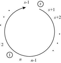
Figure 1: $\Gamma^{n,s}$ (for $n\geq 3$) - the first argument is $s$, the next $s+1$ and so on, increasing up to $n$ and then wrapping over to $1$, whence they go up to $s-1$. The circled numbers come with a minus sign in the argument, and $\Gamma^{2,2}=1$.

Appendix F Details of the component expansion for the superfields $\chi$ and $\widetilde{\chi}$ to order $g$

We present here some details of the calculation of the gluon vertices in the component Lagrangian obtained from our superspace result of section 4.

We start with the inverse transformations (96) expressing $\chi$ and $\widetilde{\chi}$ to order $g$ and substitute the truncated component expansions (97) of $\phi$ and and $\bar{\phi}$. This yields the new superfields expressed in terms of the gauge bosons as

$$\chi_{p} = \!\left\{-\frac{1}{ip_{-}}A_{p}+g\!\!\int_{qr}\!\!\delta(p-q-r)\;\Gamma_{p,q,r}\frac{1}{q_{-}r_{-}}\;A_{q}\,A_{r}+{\mathcal{O}}(g^{2})\right\}{\rm e}^{-\frac{i}{\sqrt{2}}\left(\theta\bar{\theta}\right)ip_{-}}$$

$$- \!\!\!\frac{1}{12}\langle\theta\rangle^{4}\,\left\{ip_{-}\bar{A}_{p}+g\!\!\int_{qr}\!\!\!\!\!\delta(p-q-r)\;\Gamma_{p,q,r}\left(\frac{q_{-}}{r_{-}}\;\bar{A}_{q}\,A_{r}+\frac{r_{-}}{q_{-}}\;A_{q}\,\bar{A}_{r}\right)\!+\!{\mathcal{O}}(g^{2})\right\},$$

$$\widetilde{\chi}_{p}= - \!\!\!\frac{1}{ip_{-}}\bar{A}_{p}\;{\rm e}^{\frac{i}{\sqrt{2}}\left(\theta\bar{\theta}\right)ip_{-}}-g\int_{qr}\!\!\delta(p-q-r)\left(\frac{p_{-}}{q_{-}}\;\Gamma_{-q,r,-p}\frac{1}{q_{-}r_{-}}\;\bar{A}_{q}\,A_{r}\;{\rm e}^{\frac{i}{\sqrt{2}}\left(\theta\bar{\theta}\right)i(q_{-}-r_{-})}\right.$$

$$+\left.\frac{p_{-}}{r_{-}}\;\Gamma_{-r,-p,q}\frac{1}{q_{-}r_{-}}\;A_{q}\,\bar{A}_{r}\;{\rm e}^{\frac{i}{\sqrt{2}}\left(\theta\bar{\theta}\right)i(r_{-}-q_{-})}\right)+{\mathcal{O}}(g^{2})$$

$$- \!\!\!\frac{1}{12}\langle\bar{\theta}\,\rangle^{4}\left\{ip_{-}A_{p}-g\int_{qr}\!\!\delta(p-q-r)\left(\frac{p_{-}}{q_{-}}\,\Gamma_{-q,r,-p}\,\frac{q_{-}}{r_{-}}+\frac{p_{-}}{r_{-}}\,\Gamma_{-r,-p,q}\,\frac{r_{-}}{q_{-}}\right)A_{q}\,A_{r}\right.$$

$$+{\mathcal{O}}(g^{2})\biggr{\}}$$

$$+ \!\!\!\frac{1}{12}\langle\theta\rangle^{4}\left\{g\!\int_{qr}\!\!\delta(p-q-r)\left(\frac{p_{-}}{q_{-}}\,\Gamma_{-q,r,-p}\,\frac{r_{-}}{q_{-}}+\frac{p_{-}}{r_{-}}\,\Gamma_{-r,-p,q}\,\frac{q_{-}}{r_{-}}\right)\bar{A}_{q}\,\bar{A}_{r}+{\mathcal{O}}(g^{2})\right\}$$

$$- \!\!\!\frac{1}{144}\langle\theta\rangle^{4}\langle\bar{\theta}\,\rangle^{4}\left\{g\!\int_{qr}\!\!\delta(p-q-r)\left(\frac{p_{-}}{r_{-}}\,\Gamma_{-r.-p,q}\,q_{-}r_{-}\;\bar{A}_{q}\,A_{r}\right.\right.$$

$$+\left.\frac{p_{-}}{q_{-}}\,\Gamma_{-q,r,-p}\,q_{-}r_{-}\;A_{q}\,\bar{A}_{r}\right)+{\mathcal{O}}(g^{2})\biggr{\}}\;.$$

Substituting the $\Gamma$ coefficients derived in section 3.1, $\Gamma_{+,q,r}=\frac{q_{-}r_{-}}{(q,r)}$, we get

$$\chi_{p} = \!\left\{-\frac{1}{ip_{-}}A_{p}+i\frac{2}{3}g\!\!\int_{qr}\!\!\delta(p-q-r)\;\frac{1}{(q,r)}\;A_{q}\,A_{r}+{\mathcal{O}}(g^{2})\right\}{\rm e}^{-\frac{i}{\sqrt{2}}\left(\theta\bar{\theta}\right)ip_{-}}$$ (157)

$$- \!\!\!\frac{1}{12}\langle\theta\rangle^{4}\left\{ip_{-}\bar{A}_{p}+i\frac{2}{3}g\!\!\int_{qr}\!\!\!\!\!\delta(p-q-r)\!\left(\frac{q_{-}^{2}}{(q,r)}\;\bar{A}_{q}\,A_{r}+\frac{r_{-}^{2}}{(q,r)}\;A_{q}\,\bar{A}_{r}\right)\!\!+{\mathcal{O}}(g^{2})\right\},$$

$$\widetilde{\chi}_{p}= - \!\!\!\frac{1}{ip_{-}}\bar{A}_{p}\;{\rm e}^{\frac{i}{\sqrt{2}}\left(\theta\bar{\theta}\right)ip_{-}}+i\frac{2}{3}g\int_{qr}\delta(p-q-r)\;\left(\frac{p_{-}^{2}}{q_{-}^{2}}\;\frac{1}{(q,r)}\;\bar{A}_{q}\,A_{r}\;{\rm e}^{\frac{i}{\sqrt{2}}\left(\theta\bar{\theta}\right)i(q_{-}-r_{-})}\right.$$ (158)

$$+\left.\frac{p_{-}^{2}}{r_{-}^{2}}\;\frac{1}{(q,r)}\;A_{q}\,\bar{A}_{r}\;{\rm e}^{\frac{i}{\sqrt{2}}\left(\theta\bar{\theta}\right)i(r_{-}-q_{-})}\right)+{\mathcal{O}}(g^{2})$$

$$- \!\!\!\frac{1}{12}\langle\bar{\theta}\,\rangle^{4}\left\{ip_{-}A_{p}+i\frac{4}{3}g\int_{qr}\!\!\delta(p-q-r)\;\frac{p_{-}^{2}}{(q,r)}\;A_{q}\,A_{r}+{\mathcal{O}}(g^{2})\right\}$$

$$- \!\!\!\frac{1}{12}\langle\theta\rangle^{4}\left\{i\frac{2}{3}g\!\int_{qr}\!\!\delta(p-q-r)\;\frac{p_{-}^{2}}{(q,r)}\left(\frac{q_{-}^{2}}{r_{-}^{2}}+\frac{r_{-}^{2}}{q_{-}^{2}}\right)\bar{A}_{q}\,\bar{A}_{r}+{\mathcal{O}}(g^{2})\right\}$$

$$+ \!\!\!\frac{1}{144}\langle\theta\rangle^{4}\langle\bar{\theta}\,\rangle^{4}\!\left\{i\frac{2}{3}g\!\int_{qr}\!\!\!\delta(p-q-r)\!\left(\frac{p_{-}^{2}q_{-}^{2}}{(q,r)}\;\bar{A}_{q}\,A_{r}+\frac{p_{-}^{2}r_{-}^{2}}{(q,r)}\;A_{q}\,\bar{A}_{r}\!\right)\!+\!{\mathcal{O}}(g^{2})\right\}\,.$$

To show that the new Lagrangian in terms of $\chi$ and $\widetilde{\chi}$ reduces to the MHV Lagrangian for pure Yang–Mills derived in [21, 22], we need to rewrite the new superfields in terms of the redefined component fields $B$ and $\widetilde{B}$, which make up the MHV Lagrangian for Yang–Mills. For this purpose we make use of the explicit field redefinitions derived in [23], which we reproduce here

$$A_{p} = B_{p}-g\int_{qr}\delta(p-q-r)\;\frac{p_{-}}{(q,r)}\;B_{q}\,B_{r}+{\mathcal{O}}(g^{2})\,,$$ (159)

$$\bar{A}_{p} = \widetilde{B}_{p}-g\int_{qr}\delta(p-q-r)\;\left(\frac{q_{-}^{2}}{p_{-}}\frac{1}{(q,r)}\;\widetilde{B}_{q}\,B_{r}+\frac{r_{-}^{2}}{p_{-}}\frac{1}{(q,r)}\;B_{q}\widetilde{B}_{r}\right)+{\mathcal{O}}(g^{2})\,.$$ (160)

Substituting these in (157) and (158), we obtain

$$\chi_{p} = \!\left\{-\frac{1}{ip_{-}}B_{p}-\frac{i}{3}g\!\!\int_{qr}\!\!\delta(p-q-r)\;\frac{1}{(q,r)}\;B_{q}\,B_{r}+{\mathcal{O}}(g^{2})\right\}{\rm e}^{-\frac{i}{\sqrt{2}}\left(\theta\bar{\theta}\right)ip_{-}}$$ (161)

$$- \!\!\!\frac{1}{12}\langle\theta\rangle^{4}\,\left\{ip_{-}\widetilde{B}_{p}-\frac{i}{3}g\!\!\int_{qr}\!\!\!\!\!\delta(p-q-r)\!\left(\frac{q_{-}^{2}}{(q,r)}\;\widetilde{B}_{q}\,B_{r}+\frac{r_{-}^{2}}{(q,r)}\;B_{q}\,\widetilde{B}_{r}\right)\!\!+{\mathcal{O}}(g^{2})\right\},$$

$$\widetilde{\chi}_{p} = \left\{-\frac{1}{ip_{-}}\widetilde{B}_{p}-ig\int_{qr}\!\!\delta(p-q-r)\;\left(\frac{q_{-}^{2}}{p_{-}^{2}}\frac{1}{(q,r)}\;\widetilde{B}_{q}\,B_{r}+\frac{r_{-}^{2}}{p_{-}^{2}}\frac{1}{(q,r)}\;B_{q}\,\widetilde{B}_{r}\right)\right.$$ (162)

$$+{\mathcal{O}}(g^{2})\biggr{\}}{\rm e}^{\frac{i}{\sqrt{2}}\left(\theta\bar{\theta}\right)ip_{-}}$$

$$+ \!\!\!i\frac{2}{3}g\int_{qr}\delta(p-q-r)\;\left(\frac{p_{-}^{2}}{q_{-}^{2}}\;\frac{1}{(q,r)}\;\widetilde{B}_{q}\,B_{r}\;{\rm e}^{\frac{i}{\sqrt{2}}\left(\theta\bar{\theta}\right)i(q_{-}-r_{-})}\right.$$

$$+\left.\frac{p_{-}^{2}}{r_{-}^{2}}\;\frac{1}{(q,r)}\;B_{q}\,\widetilde{B}_{r}\;{\rm e}^{\frac{i}{\sqrt{2}}\left(\theta\bar{\theta}\right)i(r_{-}-q_{-})}\right)+{\mathcal{O}}(g^{2})$$

$$- \!\!\!\frac{1}{12}\langle\bar{\theta}\,\rangle^{4}\left\{ip_{-}B_{p}+\frac{i}{3}g\int_{qr}\!\!\delta(p-q-r)\;\frac{p_{-}^{2}}{(q,r)}\;B_{q}\,B_{r}+{\mathcal{O}}(g^{2})\right\}$$

$$- \!\!\!\frac{1}{12}\langle\theta\rangle^{4}\left\{i\frac{2}{3}g\!\int_{qr}\!\!\delta(p-q-r)\;\frac{p_{-}^{2}}{(q,r)}\left(\frac{q_{-}^{2}}{r_{-}^{2}}+\frac{r_{-}^{2}}{q_{-}^{2}}\right)\widetilde{B}_{q}\,\widetilde{B}_{r}+{\mathcal{O}}(g^{2})\right\}$$

$$+ \!\!\!\frac{1}{144}\langle\theta\rangle^{4}\langle\bar{\theta}\,\rangle^{4}\left\{i\frac{2}{3}g\!\int_{qr}\!\!\delta(p-q-r)\;\left(\frac{p_{-}^{2}q_{-}^{2}}{(q,r)}\;\widetilde{B}_{q}\,B_{r}+\frac{p_{-}^{2}r_{-}^{2}}{(q,r)}\;B_{q}\,\widetilde{B}_{r}\right)+{\mathcal{O}}(g^{2})\right\}.$$

Substituting (161) and (162) in the MHV Lagrangian presented in section 4 and computing the Grassmann integrals, we reproduce the MHV Lagrangian for pure Yang–Mills.

References

• [1] J. M. Maldacena, Adv. Theor. Math. Phys. 2 (1998) 231 [arXiv:hep-th/9711200].
• [2] S. S. Gubser, I. R. Klebanov and A. M. Polyakov, Phys. Lett. B 428 (1998) 105 [arXiv:hep-th/9802109].
• [3] E. Witten, Adv. Theor. Math. Phys. 2 (1998) 253 [arXiv:hep-th/9802150].
• [4] A. Kapustin and E. Witten, “Electric-magnetic duality and the geometric Langlands program”, arXiv:hep-th/0604151.
• [5] S. Gukov and E. Witten, “Gauge theory, ramification, and the geometric Langlands program”, arXiv:hep-th/0612073.
• [6] E. Witten, “Geometric Langlands and the Equations of Nahm and Bogomolny”, arXiv:0905.4795 [hep-th].
• [7] N. Beisert et al., “Review of AdS/CFT Integrability, An Overview”, Lett. Math. Phys. vv, pp (2011) [arXiv:1012.3982].
• [8] Z. Bajnok, A. Hegedus, R. A. Janik and T. Lukowski, “Five loop Konishi from AdS/CFT”, Nucl. Phys. B 827 (2010) 426 [arXiv:0906.4062 [hep-th]].
• [9] B. S. DeWitt, “Quantum theory of gravity. III. Applications of the covariant theory”, Phys. Rev. 162 (1967) 1239.
• [10] S. J. Parke and T. R. Taylor, “An Amplitude for $n$ Gluon Scattering”, Phys. Rev. Lett. 56 (1986) 2459.
• [11] F. A. Berends and W. T. Giele, “Recursive Calculations for Processes with n Gluons”, Nucl. Phys. B 306 (1988) 759.
• [12] V. P. Nair, “A Current Algebra For Some Gauge Theory Amplitudes”, Phys. Lett. B 214 (1988) 215.
• [13] M. L. Mangano and S. J. Parke, “Multi-Parton Amplitudes in Gauge Theories”, Phys. Rept. 200 (1991) 301 [arXiv:hep-th/0509223].
• [14] L. J. Dixon, “Calculating scattering amplitudes efficiently”, TASI ’95 Lectures, arXiv:hep-ph/9601359.
Z. Bern, L. J. Dixon and D. A. Kosower, “On-Shell Methods in Perturbative QCD”, Annals Phys. 322 (2007) 1587 [arXiv:0704.2798 [hep-ph]].
• [15] F. Cachazo, P. Svrcek and E. Witten, “MHV vertices and tree amplitudes in gauge theory”, JHEP 0409 (2004) 006 [arXiv:hep-th/0403047].
• [16] E. Witten, “Perturbative gauge theory as a string theory in twistor space”, Commun. Math. Phys. 252 (2004) 189 [arXiv:hep-th/0312171].
• [17] K. Risager, “A direct proof of the CSW rules”, JHEP 0512 (2005) 003 [arXiv:hep-th/0508206].
• [18] R. Britto, F. Cachazo and B. Feng, “New Recursion Relations for Tree Amplitudes of Gluons”, Nucl. Phys. B 715 (2005) 499 [arXiv:hep-th/0412308].
R. Britto, F. Cachazo, B. Feng and E. Witten, “Direct Proof of Tree-Level Recursion Relation in Yang–Mills Theory”, Phys. Rev. Lett. 94 (2005) 181602 [arXiv:hep-th/0501052].
• [19] A. Brandhuber, B. J. Spence and G. Travaglini, “One-loop gauge theory amplitudes in ${\mathcal{N}}=4$ super Yang-Mills from MHV vertices”, Nucl. Phys. B 706 (2005) 150 [arXiv:hep-th/0407214].
• [20] Z. Bern, L. J. Dixon, D. C. Dunbar and D. A. Kosower, “One-Loop n-Point Gauge Theory Amplitudes, Unitarity and Collinear Limits”, Nucl. Phys. B 425 (1994) 217 [arXiv:hep-ph/9403226].
• [21] A. Gorsky and A. Rosly, JHEP 0601 (2006) 101 [arXiv:hep-th/0510111].
• [22] P. Mansfield, “The Lagrangian origin of MHV rules”, JHEP 0603 (2006) 037 [arXiv:hep-th/0511264].
• [23] J. H. Ettle and T. R. Morris, “Structure of the MHV-rules Lagrangian”, JHEP 0608 (2006) 003 [arXiv:hep-th/0605121].
• [24] H. Feng and Y. t. Huang, “MHV Lagrangian for ${\mathcal{N}}=4$ super Yang–Mills”, JHEP 0904 (2009) 047 [arXiv:hep-th/0611164].
• [25] L. F. Alday and J. M. Maldacena, “Gluon scattering amplitudes at strong coupling”, JHEP 0706 (2007) 064 [arXiv:0705.0303 [hep-th]].
• [26] A. Brandhuber, P. Heslop and G. Travaglini, “MHV Amplitudes in ${\mathcal{N}}=4$ Super Yang–Mills and Wilson Loops,” Nucl. Phys. B 794 (2008) 231 [arXiv:0707.1153 [hep-th]].
J. M. Drummond, J. Henn, G. P. Korchemsky and E. Sokatchev, “On planar gluon amplitudes/Wilson loops duality”, Nucl. Phys. B 795 (2008) 52 [arXiv:0709.2368 [hep-th]].
• [27] J. M. Drummond, J. Henn, G. P. Korchemsky and E. Sokatchev, “Dual superconformal symmetry of scattering amplitudes in ${\mathcal{N}}=4$ super-Yang–Mills theory”, Nucl. Phys. B 828 (2010) 317 [arXiv:0807.1095 [hep-th]].
A. Brandhuber, P. Heslop and G. Travaglini, “A note on dual superconformal symmetry of the ${\mathcal{N}}=4$ super Yang-Mills S-matrix”, Phys. Rev. D 78 (2008) 125005 [arXiv:0807.4097 [hep-th]].
• [28] R. Ricci, A. A. Tseytlin and M. Wolf, “On T-Duality and Integrability for Strings on AdS Backgrounds”, JHEP 0712 (2007) 082 [arXiv:0711.0707 [hep-th]].
N. Berkovits and J. Maldacena, “Fermionic T-Duality, Dual Superconformal Symmetry, and the Amplitude/Wilson Loop Connection”, JHEP 0809 (2008) 062 [arXiv:0807.3196 [hep-th]].
N. Beisert, R. Ricci, A. A. Tseytlin and M. Wolf, “Dual Superconformal Symmetry from AdS${}_{5}\times S^{5}$ Superstring Integrability”, Phys. Rev. D 78 (2008) 126004 [arXiv:0807.3228 [hep-th]].
• [29] L. V. Avdeev, O. V. Tarasov and A. A. Vladimirov, Phys. Lett. B 96 (1980) 94.
M. T. Grisaru, M. Rocek and W. Siegel, Phys. Rev. Lett. 45 (1980) 1063.
M. F. Sohnius and P. C. West, Phys. Lett. B 100 (1981) 245.
W. E. Caswell and D. Zanon, Nucl. Phys. B 182 (1981) 125.
P. S. Howe, K. S. Stelle and P. K. Townsend, Nucl. Phys. B 236 (1984) 125.
• [30] S. Mandelstam, Nucl. Phys. B 213 (1983) 149.
• [31] L. Brink, O. Lindgren and B. E. W. Nilsson, “The Ultraviolet Finiteness of the ${\mathcal{N}}=4$ Yang–Mills Theory”, Phys. Lett. B 123 (1983) 323.
• [32] J. M. Drummond, J. M. Henn and J. Plefka, “Yangian symmetry of scattering amplitudes in ${\mathcal{N}}=4$ super Yang–Mills theory”, JHEP 0905 (2009) 046 [arXiv:0902.2987 [hep-th]].
• [33] L. F. Alday, B. Eden, G. P. Korchemsky, J. Maldacena and E. Sokatchev, “From correlation functions to Wilson loops”, arXiv:1007.3243 [hep-th].
• [34] B. Eden, G. P. Korchemsky and E. Sokatchev, “From correlation functions to scattering amplitudes”, arXiv:1007.3246 [hep-th].
B. Eden, G. P. Korchemsky and E. Sokatchev, “More on the duality correlators/amplitudes”, arXiv:1009.2488 [hep-th].
• [35] L. Brink, O. Lindgren and B. E. W. Nilsson, “${\mathcal{N}}=4$ Yang–Mills Theory on the Light Cone”, Nucl. Phys. B 212 (1983) 401.
• [36] M. Bianchi, H. Elvang and D. Z. Freedman, “Generating Tree Amplitudes in ${\mathcal{N}}=4$ SYM and ${\mathcal{N}}=8$ SG,” JHEP 0809 (2008) 063 [arXiv:0805.0757 [hep-th]].
H. Elvang, D. Z. Freedman and M. Kiermaier, “Recursion Relations, Generating Functions, and Unitarity Sums in ${\mathcal{N}}=4$ SYM Theory”, JHEP 0904 (2009) 009 [arXiv:0808.1720 [hep-th]].
H. Elvang, D. Z. Freedman and M. Kiermaier, “Solution to the Ward Identities for Superamplitudes”, JHEP 1010 (2010) 103 [arXiv:0911.3169 [hep-th]].
H. Elvang, D. Z. Freedman and M. Kiermaier, “SUSY Ward identities, Superamplitudes, and Counterterms”, arXiv:1012.3401 [hep-th].
• [37] V. V. Khoze, “Amplitudes in the beta-deformed conformal Yang–Mills”, JHEP 0602 (2006) 040 [arXiv:hep-th/0512194].
• [38] S. Ananth, S. Kovacs and H. Shimada, “Proof of all-order finiteness for planar beta-deformed Yang–Mills”, JHEP 0701 (2007) 046 [arXiv:hep-th/0609149].
S. Ananth, S. Kovacs and H. Shimada, “Proof of ultra-violet finiteness for a planar non-supersymmetric Yang–Mills theory”, Nucl. Phys. B 783 (2007) 227 [arXiv:hep-th/0702020].
• [39] S. Ananth, L. Brink, S. S. Kim and P. Ramond, “Non-linear realization of PSU(2,2$|$4) on the light-cone”, Nucl. Phys. B 722 (2005) 166 [arXiv:hep-th/0505234].