Homogenization in a thin domain with an
oscillatory boundary
Abstract.
In this paper we analyze the behavior of the Laplace operator with Neumann boundary conditions in a thin domain of the type where the function is periodic in of period . Observe that the upper boundary of the thin domain presents a highly oscillatory behavior and, moreover, the height of the thin domain, the amplitude and period of the oscillations are all of the same order, given by the small parameter .
Résumé: Dans cet article, nous analysons le comportement de l’opérateur de Laplace avec conditions aux limites de Neumann dans un domaine fine du type lorsque la fonction est périodique dans la variable de période . On observe que la limite supérieure du domaine fine présente une comportement hautement oscillatoire et, en outre, l’ hauteur du domaine, l’amplitude et la période des oscillations sont tous du même ordre, donné par un petit paramètre .
Keywords: Thin domain, oscillatory boundary, homogenization.
1. Introduction
In this work we study the asymptotic behavior of the solutions of the Neumann problem for the Laplace operator
| (1.1) |
with , is the unit outward normal to and is the outside normal derivative. The domain is a thin domain with a highly oscillating boundary which is given by
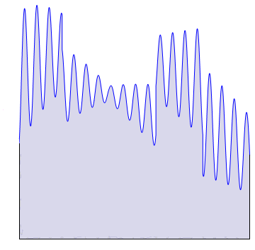
where is a function satisfying for some fixed positive constants , and such that oscillates as the parameter . We may think, for instance, that the function is of the form where are piecewise -functions defined on , is an -periodic smooth function and , see Figure 1. This includes the case where the function is a purely periodic function, for instance, but also includes the case where the function is not periodic and the amplitude is modulated by a function. As a matter of fact, we will be able to treat more general cases, see hypothesis (H) below, but to stay the general ideas in the introduction we may consider the proptotype function .
The existence and uniqueness of solutions for problem (1.1) for each is garanteed by Lax-Milgram Theorem. We are interested here in analyzing the behavior of the solutions as , that is, as the domain gets thinner and thinner although with a high oscillating boundary.
Observe that the domain is thin since and its upper boundary oscillates due to the function , (if and is not a constant function).
Since the domain is thin, “approaching” the line segment , it is reasonable to expect that the family of solutions will converge to a function of just one variable and that this function will satisfy an equation of the same type of (1.1) but in one dimension, say in with some boundary conditions, where is a second order elliptic operator in one dimension. As a matter of fact, if the function is independent of , (say or ), that is, the thin domain does not present any oscillations whatsoever:
the limit equation is given by
| (1.2) |
see for instance [10, 11]. Observe that the geometry of the thin domain enters into the limit equation through the diffusion coefficient.
Moreover, if we consider and if we assume that w- and w- (observe that a.e. and in general it is not true that ), then the limit problem is
see [2]. Observe that this case contains the previous one. If , then and , and we recover equation (1.2).
In this work we are interested in addressing the case , that is , where none of the techniques used to solve the previous ones apply. Observe that this situation is very resonant: the height of the domain, the amplitude of the oscillations at the boundary and the period of the oscillations are of the same order . Moreover we are interested in addressing not only the purely periodic case, that is, the case where the function for some -periodic smooth function but also the general case where the amplitude of the oscillation depend on in a continuous fashion, that is, in our prototype case, the situation where and are not piecewise constant, but piecewise continuous function.
The purely periodic case can be addressed by somehow standard techniques in homogenization theory, as developed in [5, 8, 12]. If where is an -periodic function and if we denote by
then the limit equation is shown to be
| (1.3) |
where
and is the unique solution of
| (1.4) |
where is the lateral boundary, is the upper boundary and is the lower boundary of , that is
We refer to [4] for a complete analysis of the purely periodic case of a nonlinear parabolic problem.
If we want to analyze now the case where the function is given by and the functions , are smooth but not necessarily constant, it is intuitively true that the limiting equation should behave like (1.3) with a diffusion coefficient depending on somehow. Actually if we look at the thin domain in a small neighborhood of a point , we will approximately see a domain with very high oscillations but locally the domain behaves like the thin domain with the function . Therefore, it is expected that if we freeze the coefficients of the limit equation in a fixed point we should recover equation (1.3). Although this intuitive argument will turn out to be true, it does not give us a complete information about the limit equation, specially, the way in which the dependence on is explicitly stated in the limit equation. For instance, it is not clear at this stage whether the limit equation should be or with or maybe where or maybe other. Observe that all these equations coincide if we consider the purely periodic case.
In order to accomplish our goal and obtain the limit equation in the general case, we propose a technique that consists in solving first the piecewise periodic case, that is, the case where the functions and are piecewise constant and then do an approximation argument to obtain the limit equation in the general case. This is a subtle argument since we are approximating first the functions and by piecewise constant functions, say , so that and obtain the limit equation for fixed, passing to the limit as . Then, in this limit equation, which will depend on , we pass to the limit as . But the limit we are interested in is taking first for fixed, so we obtain the domain given by the function , and then we pass to the limit as . But, a priori there is no garantee that these two limits commute. We will actually show that these two limits commute by proving that the solutions of problem (1.1) in two domains and , are close in the norm uniformly in when and are close. This result, which can be regarded as a domain perturbation result but uniformly in , guarantee that the two limits commute and will show that the limit problem is given as above. We remark that this domain perturbation result is not deduced from standard and known results on domain perturbation techniques since we are able to compare the solutions of an elliptic problem in two families of domains which also depend on a parameter and the way this domains depend on is not smooth at all.
We strongly believe that this technique of solving first the piecewise periodic case and then use an approximation argument, uniform in the parameter , can be used in other problems to obtain the appropriate homogenized limit for the non periodic case.
Following this agenda, we solve first the piecewise periodic case, that is, the case where the function and , are piecewise constant. We consider the points and assume that the functions and are constant in each of the interval , say , . We show that the limit equation is of the same form (1.3) in each of the intervals , that is,
| (1.5) |
where
and is the unique solution of (1.4) in the cell where
Moreover, equation (1.5) is suplemented with Neumann boundary conditions at , and with some “matching” condition at the points , , which are continuity of the function and some kind of Kirchoff type conditions, see Section 3 for details. Actually, if we look at the variational formulation of the limit equation, we obtain
| (1.6) |
where and in .
Now we will be able to pass to the limit in this equation as and obtain the limit problem:
| (1.7) |
where
and is the unique solution of (1.4) in the basic cell which depends on the variable and it is given by
Equation (1.7) is the limit equation we were looking for.
Finally, we would like to remark that although we will treat the Neumann boundary condition problem, we may also impose different conditions in the lateral boundaries of the thin domain , while preserving the Neumann type boundary condition in the upper and lower boundary. That is for problem (1.1) we may consider conditions of the Dirichlet type, , or even Robin, in the lateral boundaries , . The limit problem will preserve this boundary condition. That is, in problem (1.7) we will obtain the conditions or at and .
We describe the contents of the paper. In Section 2 we set up the notation, obtain some technical results that will be needed in the proofs and state the main result. In Section 3 we obtain the result for the piecewise periodic case. In Section 4 we show the continuous dependence result on the domain, uniform in , that will be the key argument to obtain the limit problem. In Section 5 we provide a proof of the main result. Finally, we include an Appendix where we analyze the behavior of the basic function solution of (1.4) as we perturb .
Acknowledgments. Part of this work was done while the second author was visiting the Applied Math Department at Complutense University in Madrid. He express his kind gratitude to the Department.
We would also like to thank E. Zuazua, C. Castro, M. Eugenia Pérez, M. Lobo and D. Gómez for the all the discussion and good suggestions on this problem.
2. Basic facts, notation and main result
We consider the one parameter family of functions , where , for some . We will assume the following hipothesis
-
(H)
There exist two positive constants , such that
(2.1) Moreover, the functions are of the type , where the function
(2.2) is -periodic in the second variable, that is, and piecewise with respect to the first variable, that is, there exists a finite number of points such that the function is and such that , and are uniformly bounded in and have limits when we approach and .
One important example of a function satisfying the above conditions is
where the functions , ,.., are piecewise in and the functions ,.., are all and -periodic.
We define the thin domain as
In this work we study the asymptotic behavior of the solutions of the Neumann problem for the Laplace operator
| (2.3) |
with and where is the unit outward normal to and is the outside normal derivative.
From Lax-Milgran Theorem, we have that problem (2.3) has a unique solution for each . We are interested here in analyzing the behavior of the solutions as , that is, as the domain gets thinner and thinner although with a high oscillating boundary.
To study the convergence of (2.3) in the thin oscillating domain , we consider the equivalent linear elliptic problem
| (2.4) |
where satisfies
| (2.5) |
for some independent of and now is the outward unit normal to and is given by
| (2.6) |
Observe that the equivalence between the problems (2.3) and (2.4) is obtained by changing the scale of the domain through the transformation , (see [10] for more details). Moreover, the domain is not “thin” anymore but presents very wild oscillations at the top boundary, although the presence of a high diffusion coefficient in front of the derivative with respect the second variable balance the effect of the wild oscillations.
The domain is related to the ones analyzed in the papers [6, 1, 9] but the fact that in our case we have a very high diffusion in the -direction makes our analysis and results different from these other papers.
We write for the space with the equivalent norm
given by the inner product
where is an arbitrary open set of , which may depend also on .
The variational formulation of (2.4) is find such that
| (2.7) |
Remark that the solutions satisfy an uniform a priori estimate on . In fact, taking in expression (2.7), we obtain
| (2.8) |
Consequently,
| (2.9) |
Hence, it follows from (2.5) that there exists , independent of , such that
| (2.10) |
Observe that the solutions of (2.4) can also be characterized as the minimum of a functional. That is, is the solution of (2.4) if only if
| (2.11) |
where
It follows from (2.7) with that
Hence, due to (2.5) and (2.9) we obtain
| (2.12) |
Important tools for the analysis are appropriate extension operators for functions defined in the sets . We will obtain such operator and we will be able to construct it even for more general domains that the ones like .
Hence, let us consider the following open sets:
where is an open interval, is a piecewise -function satisfying for all and and there exists such that is in the intervals . Let us define
| (2.13) |
and assume for fixed , although in general as .
Also, we denote by
Notice that .
Lemma 2.1.
With the notation above, there exists an extension operator
(where is the set of functions in which are zero in the lateral boundary ) and a constant independent of and such that
| (2.14) |
for all where and is defined in (2.13).
Proof.
Observe first that the set for all . Hence, if we have that , which implies that , we can define the operator:
Observe that this operator is obtained through a “reflection” procedure in the direction along the oscillating boundary. It is straigth forward to check that this operator satisfies (2.14).
If we are in the case where , we will need to extend first the function in the direction of negative , with a finite number of successive reflections. That is, if is defined in then we extend to the set with the reflecting along the line . This produces the function
We can continue producing these reflections inductively as follows
Choosing large enough so that , constructing and applying to the procedure by reflection in the direction along the oscillating boundary, we obtain the extension operator which satisfies (2.14). ∎
Remark 2.2.
1) This operator preserves periodicity in the variable. That is, if the function is periodic in , then the extended function is also periodic in .
2) This result can be applied to the case independent of . In particular, we can apply the extension operator to the basic cell.
Now we are in contidion to state our main result. We consider the general case, that is, the domain is given as
where the function satisfies hypothesis (H). Recall that we denote by and
where the points are given by (H).
Theorem 2.3.
Let be the solution of (2.4) with satisfying for some positive constant independent of . Assume that the function satisfies that , w-.
Then, there exists , such that, if is the extension operator constructed in Lemma 2.1, then
where depends only on the first variable, that is, , and is the unique solution of the Neumann problem
| (2.15) |
for all , where
| (2.16) |
and is the unique solution of problem
| (2.17) |
in the representative cell given by
| (2.18) |
is the lateral boundary, is the upper boundary and is the lower boundary of for all .
3. The piecewise periodic case
In this section we find the limit of the sequence given by the Neumann problem (2.4) as goes to zero for the case where the oscillating boundary is piecewise periodic.
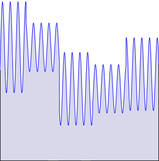
So let us consider that the family of domains satisfies (H) and morever the function is independent of the first variable in each of the domains . That is, there exist so that the function from (2.2) satisfies that for and for all . Moreover, the function is for all , there exists such that for all ; and the domain is given by
| (3.1) |
(see Figure 2). Denote also by the open rectangle and by
Observe that for and we have the extension operator constructed in Lemma 2.1.
We can show,
Theorem 3.1.
Assume that satisfies (2.5) and the function satisfies that , w-. Let be the unique solution of (2.4). Then, there exists such that if is the extension operator constructed in Lemma 2.1, we have
where in and is the unique weak solution of the Neumann problem
| (3.2) |
for all , where and are piecewise constant functions defined as follows: for all where
| (3.3) |
where is the basic cell for , that is
| (3.4) |
and for all where
and the function is the unique solution of
| (3.5) |
Remark 3.2.
If we define , then problem (3.2) is equivalent to the following:
| (3.6) |
for , where , satisfying the following boundary conditions
| (3.7) |
Here, denote the right(left)-hand side limits of at .
Proof.
Let us consider the family of representative cell , , defined by
and let be their characteristic function. We extend each periodically on the variable and denote this extension again by , for .
If we denote by the characteristic function of the set , we easily see that
| (3.8) |
Let us also denote by the rectangle , for .
Let us also consider the following families of isomorphisms given by
| (3.9) |
where
with .
Let us consider the following auxiliary problem given by
| (3.10) |
where is the lateral boundary, is the upper boundary and is the lower boundary of .
Taking the isomorphism (3.9) and the family of extension operators
defined by Lemma 2.1 with independent of and , see Remark 2.2, we define the function
Notice that this function is defined in and it is well defined. For fixed and for for some then there exists a unique such that . Observe that and that .
We introduce now the vector defined by
| (3.11) |
Since and we have that
for and , for .
It follows from definition of that the functions and satisfy
| (3.12) |
where
In fact, by (3.10) we have
on for . Moreover,
Therefore, multiplying (3.12) by a test function with in neighborhood of the set and integrating by parts, we obtain
That is
| (3.13) |
| (3.14) | |||||
Using that we cancel the appropriate terms and obtain
| (3.15) |
On the other hand, we have obtained before the weak formulation of problem (2.4), that is
| (3.16) |
Now we need to pass to the limit in (3.15) and (3.16). In order to accomplish this we need to write both expressions as integrals in the same domain. For this, we will use the extension constructed in Lemma 2.1, the standard extension by zero, that we denote by , and the characteristic function of as follows:
| (3.17) |
| (3.18) |
Observe that in this last equality we have taken and the term including partial derivatives with respect to do not appear.
We want to pass to the limit in the expressions above, (3.17) and (3.18) . In order to accomplish this, we pass to the limit in the different functions that form the integrands.
(a). Limit of .
From (3.8), we have for ,
| (3.19) |
Observe that the limit does not dependent on the variable , although it depends on . Moreover, we can get the area of the open set with the formula
| (3.20) |
Also, from (3.19) we have that
a.e. and for all . So, due to
we can get by Lebesgue’s Dominated Convergence Theorem that
| (3.21) |
where for , .
(b). Limit in the tilde functions
Since is uniformly bounded, we get from (2.8) that there exists independent of such that
| (3.22) |
Then, we can extract a subsequence, still denoted by , and , such that
| (3.23) |
as for some and .
Moreover, since independent of , we have and therefore, the function defined by
| (3.24) |
satisfies that . Hence, via subsequences, we have the existence of a function such that
| (3.25) |
(c). Limit in the extended functions
Using the a priori estimate (2.8), the fact that and using the results from Lemma 2.1 on the extension operator we get that
| (3.26) |
where is a positive constant independent of given by estimate (3.22) and Lemma 2.1. Then, we can extract a subsequence, still denoted by and a function , such that
| (3.27) |
A consequence of the limits (3.27) is that does not depend on the variable . More precisely,
| (3.28) |
In fact, for and for all , we have by (3.27) that
which implies that does not depend on . Morever, since the rectangle for all and we have from (3.27) that and therefore .
Also, we note that . Thus, it follows from (3.21), (3.23) and (3.27) that we have the following relationship between and
| (3.29) |
(d). Limit in .
With the definition of , we have for all ,
and so,
Similarly,
and
Also, we have
for all and
Then, we can conclude
| (3.30) |
and
(e). Limit of
Let be the extension by zero of the vector to the whole . We can obtain by the Average Theorem that
| (3.31) |
where is the characteristic function of .
Now, by the convergences shown in (a)-(e) above, we can pass to the limit in (3.17) and in (3.18). We obtain, for all ,
Observe that . Consequently, we have
| (3.33) |
for all . From (3.18), we get
| (3.34) |
In particular, via iterated integration and (3.34), we get
| (3.35) |
Taking in (3.34), we get
| (3.36) |
Hence, it follows from (3.33) and (3.36) that, for all ,
| (3.37) |
where we have performed an integration by parts to obtain the last integral. Observe that this integration by parts can be performed since and does not depend on in each of the domains . Hence, if we define
and we denote by
and performing an iterated integration in (3.37) we get
which implies that
| (3.38) |
Plugging this last equality in (3.35) we get
| (3.39) |
∎
4. A domain dependence result
In this section we are going to analyze how the solutions of (2.4) depend on the domain and more exactly on the function . As a matter of fact we will show a continuous dependence result with respect to the functions .
More precisely, assume and are piecewise continuous functions satisfying (2.1) and consider the associated oscillating domains and given by
Let and be the solutions of the problem (2.4) in the oscillating domains and respectively with . Then we have the following result:
Theorem 4.1.
There exists a positive real function such that
| (4.1) |
with as uniformly for all
-
•
;
-
•
piecewise functions and with and
-
•
, .
Remark 4.2.
The important part of this result is that the function does not depend on . Only depends on and .
To prove this theorem, we use the fact that and are minimizers of the quadratic forms
| (4.2) |
That is, we have
In order to prove Theorem 4.1 we will need to consider the minimizer of the functionals , , and plug them in the other functional. For this, we need to transform the function into a function defined in and the function into a function defined in . One possibility is to use some kind of extension operator as the one we have constructed in Section 2. But the problem with this approach is that the norm of the extension operators will depend on the derivatives of the function and and therefore it will be very unlikely to prove a results that will depend only on the norm of .
In order to transform the function (resp. ) into a function defined in (resp. ), we construct the following operators:
| (4.3) |
where
and is an arbitrary open set.
We also consider the following norm in
| (4.4) |
and we can easily see that
| (4.5) |
and
| (4.6) |
We have the following preliminary result about the behavior of the solutions near of the oscillating boundary.
Lemma 4.3.
Then exists a positive constant independent of such that
for all .
Proof.
Since , we have . So, we obtain,
where we have used (4.5), (4.6). Moreover,
where we have used that satisfies the variational formulation (2.7) with .
Consequently, it follows from (LABEL:EQ1) that
Hence, we obtain
| (4.8) |
We are in conditions now to proof the main result of this section.
So we will concentrate in the first term of (4.1). Therefore,
But from (4.5) and (4.6) we get
| (4.15) |
Moreover
but from Lemma 4.3,
Also,
Hence, putting all this information together, we get
Therefore
| (4.16) |
5. The General Case
We provide now a proof of the main result, Theorem 2.3.
Proof.
From estimate (2.10) and (2.14) we derive
where is a positive constant independent of . Hence, there exists and a subsequence, still denoted by , such that
| (5.1) |
It follows from (5.1) that on .
We will show that satisfies the Neumann problem (2.15). To do this, we use a discretization argument.
Let us fix a parameter small enough and consider a function with the property that for all and such that the function satisfies hypothesis (H) and is piecewise periodic as described in Section 3. To construct this function, we may proceed as follows. The function is uniformly in each of the domains and it is also periodic in the second variable. In particular, for small enough and for a fixed we have that there exists a small interval with depending only on such that for all and for all . This allows us to select a finite number of points: such that and therefore, defining for all we have that and for all . This construction can be done for all .
In particular, if we rename all the points constructed above by (and observe that ), the function with , and is and -periodic.
We denote by and consider the domains
Since satisfies the hyphoteses of the Lemma 2.1, there exists an extension operator
satisfying the uniform estimate (2.14) with .
Since with , then if we extend this function by 0 outside and denoting the extended function again by and using that , we have that and by hypothesis, we have that w-.
Therefore, it follows from Theorem 3.1 that for each fixed, there exist such that the solutions of (2.4) in satisfy
| (5.2) |
where on is the unique solution of the Neumann problem
| (5.3) |
where and are strictly positive functions, locally constant, given by
| (5.4) |
where
| (5.5) |
The function is the unique solution of (3.5) in the representative cells defined in (3.4) for all .
Now, we pass to the limit in as . To do this, we consider the functions and defined in and the functions and defined in (2.16). We have that and converge to and uniformly in . The uniform convergence of to in it follows from Proposition A.1 proved in the Appendix. The uniform convergence of to follows from the uniform convergence of to as .
Since we have the uniform convergence of and to and respectively, we have by [5, p. 8] or [8, p. 1] the following limit variational formulation: to find such that
| (5.6) |
for all .
To finish the proof, we need to show that in , where is the function obtained in (5.1).
Let us consider the open square which satisfies for all and small enough. Observe that and therefore, to show that it is enough to show that . Hence, adding and substracting the appropriate functions and with the triangular inequality,
| (5.8) |
for all and .
Now, let be a positive small number. From (5.7) and from Theorem 4.1, we can choose a fixed and small such that and uniformly for all . Now, from (5.2) for this particular value of , we can choose small enough such that for . Moreover, from (5.1) we have that there exists such that for all . Hence with applied to (5.8), we get . Since is arbitrarilly small, then . ∎
Appendix A A perturbation result in the basic cell.
In the proof of the main result in Section 5 we have used the convergence of , where in the interval , and , are defined by (5.5) and (2.16), respectively. In order to proof such a convergence we need to analyze how the function , solution of
| (A.1) |
on the representative cell
| (A.2) |
depends on the function .
We will consider the following class of admissible functions
| (A.3) |
and we will denote by and the basic cell (A.2) and the solution of (A.1) for a particular . Observe that for each , we have the extension operator as constructed in Lemma 2.1, which will satisfy with , but independent of , and therefore this constant can be chosen the same for all .
For each , we can consider the basic cell defined by (A.2). Here, we proceed as [2, p. 84] and [10], we begin by making the following transformation on the domain
where . The Jacobian matrix for this transformation is
and observe that its determinant is given by .
Using , we can show that problem (A.1) in is equivalent to
| (A.4) |
where
That is, we have that is the solution of (A.1) in if and only if satisfies equation (A.4) in .
Moreover, if we define
then, is the unique solution of
| (A.5) |
Also, we have that the variational formulation of problem (A.5) is given by the bilinear form
where is given by
with the norm. Hence, we have that is the solution of (A.1) in if and only if
| (A.6) |
satisfies
| (A.7) |
Observe also that the bilinear form associated to problem (A.1) in is given by
and the weak formulation is given by
As a matter of fact, we will be able to show the following:
Proposition A.1.
Let us consider the family of admissible functions for some constant , where is defined in (A.3).
Then, for each there exists such that if with , then
| (A.8) |
Proof.
Obviously (A.9) follows straightforward from (A.8), the relation between and stated in (A.6), the definition of in (A.10) and the fact that and are close in the -metric, and in particular in the uniform norm.
Hence, we need to show (A.8). For this let and be bilinear forms associated to the variational formulation of (A.5) for and respectively. We can get the following estimate
| (A.11) | |||||
Since
we have
Then, due to (A.11), we get
| (A.12) |
where the constant depends on , and and therefore it can be chosen the same constant for all .
Now, since is a coercive bilinear form in (observe that we have imposed the condition in ) then, there will exist a constant such that . But, to simplify, if we denote by and , we will have
But using appropriate trace theorems in , the fact that , so that they are uniformly bounded in (and therefore for a constant depending only on ), then, we easily get that , where we have used that we have a uniform bound of for all , which is easily obtained from the variational formulation (A.7) and the fact that . This shows (A.8) and we conclude the proof of the result. ∎
References
- [1] Y. Amirat, O. Bodart, U. de Maio, A. Gaudiello, “Asymptotic Approximation of the solution of the Laplace equation in a domain with highly oscillating boundary”, SIAM J. Math. Anal. 35, 1598-1616 (2004)
- [2] J. M. Arrieta, Spectral properties of Schrödinger operators under perturbations of the domain, Ph.D. Thesis, Georgia Institute of Technology, (1991)
- [3] J. M. Arrieta and M. C. Pereira, “Elliptic problems in thin domains with highly oscillating boundaries”, Bol. Soc. Esp. Mat. Apl. 51, pp:17-24 (2010).
- [4] J. M. Arrieta, A. N. Carvalho, M. C. Pereira and R. P. da Silva; “Nonlinear parabolic problems in thin domains with a highly oscillatory boundary”, Submitted.
- [5] A. Bensoussan, J. L. Lions and G. Papanicolaou, Asymptotic Analysis for Periodic Structures, North-Holland Publishing Company (1978).
- [6] R. Brizzi, J.P. Chalot, “Boundary homogenization and Neumann boundary problem” Ricerce di Matematica XLVI, 2 (1997) 341-387
- [7] V. Burenkov, P.D. Lamberti, “Spectral Stability of general non-negarive self-adjoint operators with applications to Neumann-type operators”, J. Differential Equations 233 (2007), 345-379
- [8] D. Cioranescu and J. Saint Jean Paulin; Homogenization of Reticulated Structures, Springer Verlag (1980).
- [9] A. Damlamian, K. Pettersson, “Homogenization of oscillating boundaries” , Discrete and Continuous Dynamical Systems 23, (2009), 197-219
- [10] J. K. Hale and G. Raugel, “Reaction-diffusion equation on thin domains”, J. Math. Pures and Appl. (9) 71, no. 1, 33-95 (1992).
- [11] G. Raugel; Dynamics of partial differential equations on thin domains in Dynamical systems (Montecatini Terme, 1994), 208-315, Lecture Notes in Math., 1609, Springer, Berlin, 1995.
- [12] E. Sánchez-Palencia, Non-Homogeneous Media and Vibration Theory, Lecture Notes in Physics 127, Springer Verlag (1980)
- [13] L. Tartar; Problèmmes d’homogénéisation dans les équations aux dérivées partielles, Cours Peccot, Collège de France (1977).
- [14] L. Tartar, “Quelques remarques sur l’homegénéisation”, Function Analysis and Numerical Analysis, Proc. Japan-France Seminar 1976, ed. H. Fujita, Japanese Society for the Promotion of Science, 468-482 (1978).