Computation for Supremal Simulation-Based Controllable and Strong Observable Subautomata

Abstract

Bisimulation relation has been successfully applied to computer science and control theory. In our previous work, simulation-based controllability and simulation-based observability are proposed, under which the existence of bisimilarity supervisor is guaranteed. However, a given specification automaton may not satisfy these conditions, and a natural question is how to compute a maximum permissive sub-specification. This paper aims to answer this question and investigate the computation of the supremal simulation-based controllable and strong observable subautomata with respect to given specifications by the lattice theory. In order to achieve the supremal solution, three monotone operators, namely simulation operator, controllable operator and strong observable operator, are proposed upon the established complete lattice. Then, inequalities based on these operators are formulated, whose solution is the simulation-based controllable and strong observable set. In particular, a sufficient condition is presented to guarantee the existence of the supremal simulation-based controllable and strong observable subautomata. Furthermore, an algorithm is proposed to compute such subautomata.

I INTRODUCTION

Bisimulation relation was introduced in [1] as a behavioral equivalence relationship between two dynamical systems, and since then it has been used widely in the study of discrete event systems (DESs) [2], linear systems [3], probabilistic systems [4], and hybrid systems [5]. Bisimulation provides a stronger equivalence than the extensively studied language equivalence [9]. It is known that the language generated by two bisimilar systems are equivalent, but the systems possessing the same language might not be bisimilar. Moreover, two bisimilar systems have equivalent reachability properties, or more generally, preserve properties specified in terms of temporal logic such as CTL* [12]. Therefore, the bisimilarity control that aims to achieve a bisimulation equivalence between controlled system and specification has attracted lots of attentions these years.

Komenda and Schuppen characterized the language controllability and observability in terms of partial bisimulation by using coalgebra for supervisory control of DESs under partial observation [6]. Tabuada investigated the controller synthesis problem of affine systems for bisimulation equivalence [7] and extended it to various systems including discrete-event systems, nonlinear control systems, behavioral systems, and hybrid systems by means of category theory [8]. In Zhou's work [13] and our previous work [14], the problem addressed is to design a supervisor to execute the control action to achieve the bisimulation relation between supervised system and specification, where plant and specification are generally described as nondeterministic automata. In Zhou's work [13], a small model theorem is established to show that the supervisor exists if and only if it exists over the power set of Cartesian product of system and specification state spaces.

In our previous work [14], a different framework is proposed to characterize the existence of the supervisor. The supervisor exists if and only if the specification is simulation-based controllable under full observation. As for the partial observation case, the specification should be both simulation-based controllable and simulation-based observable to ensure the existence of the supervisor. However, in most situations, a given specification does not satisfy those conditions. Then, a natural question is how to compute a maximum permissive sub-specification. Here, we would like to calculate the supremal simulation-based controllable and strong observable subautomata. Please note that the existing work for the calculation of supremal controllable/normal sublanguages are all based on the language controllability/normality [16], [17]. To our best knowledge, there is no work considering the computation of the supremal subautomata under simulation-based controllability and simulation-based observability, where the specifications are given as automata instead of languages.

This paper aims to answer this question and investigate the computation of the supremal simulation-based controllable and strong observable subautomata with respect to given specifications by the lattice theory. Some preliminary results on the computation of the supremal simulation-based controllable subautomata under full observations were presented in [10]. In this paper, we will calculate the supremal simulation-based controllable and strong observable subautomata for the partial observation case. In order to achieve the supremal solution, three monotone operators, namely simulation operator, controllable operator and strong observable operator, are proposed upon the established complete lattice. Then, inequalities based on these three operators are formulated, whose solution is the simulation-based controllable and strong observable set. In particular, a sufficient condition is presented to guarantee the existence of the supremal simulation-based controllable and strong observable subautomata. Furthermore, an algorithm is proposed to compute such subautomata.

This note is organized as follows. Section 2 gives the preliminary. Section 3 reviews the works that have been done under full observation. Section 4 studies the computation of the supremal simulation-based controllable and strong observable subautomata under partial observation. An illustrative example is provided in Section 5. The note concludes with section 6.

II Preliminary

II-A Discrete Event System

A DES is modeled as an automaton $G=(X,\Sigma,x_{0},\alpha,X_{m})$, where $X$ is the set of states, $\Sigma$ is a finite set of events, $\alpha:X\times\Sigma\rightarrow 2^{X}$ is the transition function, $x_{0}$ is the initial state, $X_{m}\subseteq X$ is the set of marked states. $\Gamma:X\rightarrow 2^{\Sigma}$ is the active function and $\Gamma(x)$ is the active event set at state $x$. Let $\Sigma^{*}$ be the set of all finite strings over $\Sigma$, including the empty string $\epsilon$. Then the transition function $\alpha$ can be extended to $\alpha:X\times\Sigma^{*}\rightarrow 2^{X}$ in the nature way [9]. The language generated by $G$ is defined as $L(G)=\{s\in\Sigma^{*}\mid\alpha(x_{0},s)$ is defined$\}$. The event set can be partition into $\Sigma$ = $\Sigma_{uc}\dot{\cup}\Sigma_{c}$, where $\Sigma_{uc}$ is the set of uncontrollable events and $\Sigma_{c}$ is the controllable event set. It can be also partitioned into $\Sigma$ = $\Sigma_{uo}\dot{\cup}\Sigma_{o}$, where $\Sigma_{uo}$ is the set of unobservable events and $\Sigma_{o}$ is the set of observable events. Given an event string $s\in\Sigma^{*}$, $|s|$ is the length of the string and $s(i)$ is the $i^{th}$ event of this string, where $1\leq i\leq|s|$. When a string of events occurs, the sequence of observable events is filtered by a projection $P$: $\Sigma^{*}\rightarrow\Sigma_{o}^{*}$, which is defined inductively as follows: $P(\epsilon)=\epsilon$, for $\sigma\in\Sigma$ and $s\in\Sigma^{*}$, $P(s\sigma)=P(s)\sigma$ if $\sigma\in\Sigma_{o}$, otherwise, $P(s\sigma)=P(s)$. The accessible operator $Ac$ is used to remove the states which are not accessible from the initial state, and it is defined as below.

Definition 1

Given an automaton $G=(X,\Sigma,x_{0},\alpha,X_{m})$, the accessible operator on G is defined as:

$$Ac(G)=(X_{ac},\Sigma,x_{0},\alpha_{ac},X_{acm}),$$

where $X_{ac}=\{x\in X\mid x\in\alpha_{ac}(x_{0},s)$, where $s\in\Sigma^{*}$ }, $X_{acm}=X_{m}\cap X_{ac}$, $\alpha_{ac}$: $X_{ac}\times\Sigma\rightarrow X_{ac}$ is a transition function, and for any $x\in X_{ac}$ and $e\in\Sigma$, $\alpha_{ac}(x,e)=\{y\in X_{ac}\mid y\in\alpha(x,e)\}$.

Further, the concept of subautomaton is introduced and a subautomaton operator is proposed to construct a subautomaton from a given state set.

Definition 2

Given an automaton $G=(X,\Sigma,x_{0},\alpha,X_{m})$, the subautomaton of $G$ is defined as $G_{1}=(X_{1},\Sigma_{1},x_{0},\alpha,X_{m1})$, where $X_{1}\subseteq X$, $X_{m1}\subseteq X_{m}$, and $\alpha_{1}$ = $\alpha\mid X_{1}\times\Sigma\rightarrow X_{1}$.

The notation $\alpha\mid X_{1}\times\Sigma\rightarrow X_{1}$ means that we are restricting $\alpha$ to the smaller domain of the states $X_{1}$. The subautomaton of $G$ picks its states and marked states from the corresponding sets in $G$.

Definition 3

Given an automaton $R=(Q,\Sigma,q_{0},\delta,Q_{m})$, the subautomata operator is defined as:

$$Rc(Z)=Ac(Q_{rc},\Sigma,q_{0},\delta_{rc},Q_{rcm}),$$

where Z $\subseteq Q\times X$, $Q_{rc}$ = {$q\in Q\mid(q,x)\in Z$}, $Q_{rcm}$ = $Q_{m}\cap Q_{rc}$, and $\delta_{rc}=\delta\mid Q_{rc}\times\Sigma\rightarrow Q_{rc}$.

By this subautomata operator, we can construct a subautomata of the original automata $R$ from a set $Z$, whose elements are the state pairs of $R$ and $G$. In addition, the state set $Q_{rc}$ of this subautomata is a subset of the corresponding state set $Q$ of $R$ and the transition function of this subautomata restricts $\delta$ to a smaller domain of the states $Q_{rc}$.

Then, simulation relation is used to describe the equivalence between automata as follows.

Definition 4

Let $G_{1}=(X_{1},\Sigma,x_{01},\alpha_{1},X_{m1})$ and $G_{2}=(X_{2},\Sigma,x_{02},\alpha_{2},X_{m2})$ be two automata. $G_{1}$ is said to be simulated by $G_{2}$, denoted by $G_{1}\prec_{\phi}G_{2}$, if there is a binary relation $\phi$ $\subseteq$ $X_{1}\times X_{2}$ such that $(x_{01},x_{02})\in\phi$ and for each $(x_{1},x_{2})\in\phi$,

(1) $x_{1}^{{}^{\prime}}\in\alpha_{1}(x_{1},\sigma)$, where $\sigma\in\Sigma\Rightarrow\exists x_{2}^{{}^{\prime}}\in\alpha_{2}(x_{2},\sigma)$ such that $(x_{1}^{{}^{\prime}},x_{2}^{{}^{\prime}})\in\phi$.

(2) $x_{1}\in X_{m1}$, then $x_{2}\in X_{m2}$.

If $G_{1}\prec_{\phi}G_{2}$, $G_{2}\prec_{\phi}G_{1}$, and $\phi$ is symmetric, $\phi$ is a bisimulation relation between $G_{1}$ and $G_{2}$, denoted by $G_{1}\simeq_{\phi}G_{2}$. We sometimes omit the subscript $\phi$ from $\prec_{\phi}$ or $\simeq_{\phi}$ when it is clear from the context. Moreover, the main result of [14] is as below.

Theorem 1

Given a plant $G=(X,\Sigma,\alpha,x_{0},X_{m})$, a specification $R=(Q,\Sigma,\delta,q_{0},Q_{m})$ and a projection $P$, assume that $L(R)$ is language controllable and language observable. Then, there exists a simulation relation $\Phi\subseteq Q\times X$ and a $P$-supervisor $S_{P}$ such that $S_{P}^{\Phi}/G\simeq R$ and $S_{P}^{\Phi}/G$ is $\Sigma_{uc}$-consistent if and only if $R$ is simulation-based controllable and simulation-based observable.

The simulation-based controllability and simulation-based observability are defined as below.

Definition 5

Given a plant $G=(X,\Sigma,x_{0},\alpha,X_{m})$ and a specification $R=(Q,\Sigma,q_{0},\delta,Q_{m})$, $R$ is simulation-based controllable with respect to $G$ and $\Sigma_{uc}$ if it satisfies:

(1) (Simulation Condition) There is a simulation relation $\phi$ such that $R\prec_{\phi}G$.

(2) (Controllable Condition) ($\forall$ $s\in L(R)$)($\forall$ $q$ $\in$ $\delta(q_{0},s)$)($\forall$ $\sigma\in\Sigma_{uc}$)[$s\sigma\in L(G)\Rightarrow\delta(q,\sigma)\neq\emptyset]$.

The set $Q_{1}\times X_{1}\subseteq Q\times X$ is said to be a simulation-based controllable set if $Q_{1}\times X_{1}$ is a simulation relation from $R$ to $G$ and $Rc(Q_{1}\times X_{1})$ satisfies the controllable condition.

Definition 6

Given a plant $G=(X,\Sigma,x_{0},\alpha,X_{m})$ and a specification $R=(Q,\Sigma,q_{0},\delta,Q_{m})$. $R$ is said to be simulation-based observable with respect to $G$, $\Sigma_{c}$ and $P$, if it satisfies:

(1) (Simulation Condition) There is a simulation relation $\phi$ such that $R\prec_{\phi}G$.

(2) (Observable Condition) $\forall s$, $s^{\prime}\in L(R)$ with $P(s)=P(s^{\prime})$ $(\forall q\in\delta(q_{0},s))$ $(\forall\delta\in\Sigma_{c})$ $[s^{\prime}\sigma\in L(R)$ and $s\sigma\in L(G)\Rightarrow\delta(q,\sigma)\neq\emptyset$].

Simulation-based controllability and simulation-based observability implies language controllability and language observability, but the reverse does not hold.

II-B Lattice Theory

Definition 7

Consider a set $X$ and a relation $R\subseteq X\times X$ over $X$. $R$ is reflexive if for each $x\in X$, $(x,x)\in R$; it is antisymmetric if $(x,y)\in R$ and $(y,x)\in R$ implies $x=y$; it is transitive if $(x,y)\in R$ and $(y,z)\in R$ implies that $(x,z)\in R$. The partial order relation, denoted by $\leq$, over $X$ is a reflexive, antisymmetric and transitive relation. The pair $(X,\leq)$ is a poset.

Definition 8

Consider a set $X$ and $Y\subseteq X$. $x\in X$ is said to be the supremal of $Y$, denoted by $supY$ or $\sqcup Y$, if it satisfies : (1) $\forall y\in Y$: $y\leq x$, (2) $[\forall y\in Y:y\leq z]\Rightarrow[x\leq z]$. $x$ is said to be the infimal of $Y$, denoted by $infY$ and $\sqcap Y$, if it satisfies: (1) $\forall y\in Y$: $x\leq y$ (2) $\forall z\in X$ : $[\forall y\in Y:z\leq y]\Rightarrow[z\leq x]$. The poset $(X,\leq)$ is called a lattice if $supY$, $infY\in X$ for any finite $Y$. If $supY,infY\in X$ for arbitrary $Y\subseteq X$, then $(X,\leq)$ is called a complete lattice.

A poset may be a lattice, but it may have a set $Y$ of infinite size for which $infY$ or $supY$ may not exist. However, $infY$ and $supY$ exist for any $Y\subseteq X$ on a complete lattice. Moreover, monotone functions and disjunctive functions are defined over a complete lattice $(X,\leq)$.

Definition 9

A function $f:X\rightarrow X$ is said to be monotone if for any $x,y\in X$ : $[x\leq y]\Rightarrow[f(x)\leq f(y)]$. $f$ is said to be disjunctive if for any $Y\subseteq X:f(\sqcup_{y\in Y}Y)=\sqcup_{y\in Y}f(y)$.

Furthermore, the following lemmas are introduced to obtain the supremal solution of the system of inequalities [11].

Lemma 1

Consider the system of inequalities {$f_{i}(x)\leq g_{i}(x)$}_i≤n over a compete lattice (X, $\leq$). Let Y = {$y\in X\mid\forall i\leq n:f_{i}(y)\leq g_{i}(y)$} be the set of all solutions of the system of inequalities and $Y_{1}$ = {$y\in X\mid h_{1}(y)=y$} be the set of all fixed points of $h_{1}$, where $h_{1}=\sqcap_{i\leq n}f_{i}^{\bot}(g_{i}(y))$ and $f_{i}^{\bot}(g_{i}(y))$ is the supremal solution of $f_{i}(x)\leq g_{i}(x)$. If $f_{i}$ is disjunctive and $g_{i}$ is monotone, then $supY\in Y$, $supY_{1}\in Y_{1}$, and $supY=supY_{1}$.

Lemma 2

Consider the inequalities {$f_{i}(x)\leq g_{i}(x)\}_{i\leq n}$ and $Y=\{y\in X\mid\forall i\leq n:f_{i}(y)\leq g_{i}(y)$}. If $f_{i}$ is disjunctive and $g_{i}$ is monotone, $supY$ can be obtained by iterative computation: $y_{0}=supX$, $\forall k\geq 0,y_{k+1}=h_{1}(y_{k})$ until $y_{m+1}=y_{m}=supY$.

In this note, we focus on the computation of the supremal simulation-based controllable and strong observable subautomaton for the specification, which is not simulation-based controllable and observable.

III Full Observation

In this section, we establish a complete lattice over which the constructed simulation operator, controllable operator and their properties are reviewed [10].

Definition 10

Given a plant $G=(X,\Sigma,x_{0},\alpha,X_{m})$ and a specification $R=(Q,\Sigma,q_{0},\delta,Q_{m})$, the poset is defined as ($2^{Q\times X},\subseteq$).

It can be seen that this power set lattice ($2^{Q\times X},\subseteq$) is built upon the state pairs from $R$ and $G$ and it is a complete lattice [11]. Thus, supremal and infimal defined with respect to a compete lattice are unique.

Remark 1

An alternative poset can be a prelattice $(\mathcal{S},\prec)$, where $\mathcal{S}$:= {$S^{\prime}~{}|~{}(S^{\prime}\prec R)\wedge(S^{\prime}$ is simulation-based controllable and strong observable) } is a set of automata and $\prec$ is a simulation relation. However, the supremal solution with respect to the prelattice $(\mathcal{S},\prec)$ is not unique because this simulation relation over $\mathcal{S}$ is a preorder, which is transitive, reflexive but not anti-symmetric.

Next, we introduce several operators defined over ($2^{Q\times X},\subseteq$).

Definition 11

The simulation operator $F_{s}:2^{Q\times X}\rightarrow 2^{Q\times X}$ defined by $(q,x)\in F_{s}(Z)$, for $Z\subseteq Q\times X$, if the following conditions are satisfied:

1. $(q,x)\in Z$.

2. $q^{{}^{\prime}}\in\delta(q,\sigma)$ $\Rightarrow$ $[\exists x^{{}^{\prime}}\in\alpha(x,\sigma)]$ $[(q^{{}^{\prime}},x^{{}^{\prime}})\in Z]$.

3. $q\in Q_{m}$ $\Rightarrow$ $x\in X_{m}$.

The simulation operator evolves from a similar operator in [15] and it has following properties. Their proofs can be found in [10].

Proposition 1

Given a plant $G=(X,\Sigma,x_{0},\alpha,X_{m})$ and a specification $R=(Q,\Sigma,q_{0},\delta,Q_{m})$, $\phi$ is a simulation relation from $R$ to $G$ if and only if $\phi\subseteq F_{s}(\phi)$ and $(q_{0},x_{0})\in\phi$.

Proposition 2

Given a plant $G=(X,\Sigma,x_{0},\alpha,X_{m})$, a specification $R=(Q,\Sigma,q_{0},\delta,Q_{m})$ and the sets $Z,Z^{\prime}\subseteq Q\times X$, $F_{s}(Z)\subseteq F_{s}(Z^{{}^{\prime}})$ if $Z\subseteq Z^{{}^{\prime}}$.

Theorem 2

Given a plant $G=(X,\Sigma,x_{0},\alpha,X_{m})$ and a specification $R=(Q,\Sigma,q_{0},\delta,Q_{m})$, the supremal simulation relation is the maximal fixed-point $Z$ of the operator $F_{s}$ if $(q_{0},x_{0})\in Z$, where $Z\subseteq Q\times X$. Moreover,

$$F_{s}(Z)=\lim_{i\rightarrow\infty}F_{s}^{i}(Q\times X),$$

where $F_{s}^{0}(Q\times X)=Q\times X$ is an identity function, and for each $i\geq 0$, $F_{s}^{i+1}(Q\times X)=F_{s}(F_{s}^{i}(Q\times X))$.

Before presenting the controllable operator, we introduce the following concepts.

Definition 12

Given an automaton $G_{1}=(X_{1},\Sigma_{1},x_{0},\alpha_{1},X_{1m},\Gamma_{1})$ and a state $x\in X_{1}$, the string set of $x$, denoted by $S_{x}$, is defined as $S_{x}=\{s\in\Sigma^{*}~{}|~{}x\in\alpha_{1}(x_{0},s)\}$. The nondeterministic state set of $x$, denoted by $X_{x}$, is defined as $X_{x}=\{x\in X_{1}~{}|~{}x\in\alpha_{1}(x_{0},s),s\in S_{x}\}$. Further, we define the nondeterministic active event set of the state $x$, denoted by $\Gamma_{n}(x)$, as $\Gamma_{n}(x)=\cup_{x_{1}\in X_{x}}\Gamma_{1}(x_{1})$.

We can obtain all the strings that can reach $x$ from $x_{0}$ through $S_{x}$ and all the states that are reachable from $x_{0}$ with the strings in $S_{x}$ by $X_{x}$. Besides, $\Gamma_{n}(x)$ is a union of the active event set of the states in $X_{x}$. Next, we propose the following notion to guarantee the existence of the supremal simulation-based controllable subautomata.

Definition 13

Given a plant $G$ and a specification $R=(Q,\Sigma,q_{0},\delta,Q_{m})$, $R$ is said to be calculable for the supremal simulation-based controllable subautomaton with respect to $G$ if it satisfies:

$$(\forall q\in Q_{M})(\forall s\in S_{q})(\forall\sigma\in\Sigma_{uc})[s\sigma\in L(G)\Rightarrow\delta(q,\sigma)\neq\emptyset]$$

where $Q_{M}=\{q\in Q~{}|~{}|S_{q}|\geq 2\}$.

Before presenting the controller operator, the simulation-based controllable product is established.

Definition 14

Given a plant $G=(X,\Sigma,x_{0},\alpha,X_{m})$ and a specification $R=(Q,\Sigma,q_{0},\delta,Q_{m})$, the simulation-based controllable product of $R$ and $G$ is an automaton:

$$R\times_{sc}G=Ac(Q\times X\cup\{(q_{v},x_{v})\},\Sigma,q_{0}\times x_{0},\gammaup_{sc},Q_{m}\times X_{m})$$

where

$$\ \gammaup_{sc}((q,x),\sigma)=\left\{{\begin{array}[]{*{20}c}(q_{v},x_{v})&{\sigma\in(\Sigma_{uc}\cap(\Gamma_{n}(x)-\Gamma(q))};\\ (\delta(q,\sigma),\alpha(x,\sigma))&{\sigma\in\Gamma(x)\cap\Gamma(q)};\\ undefined&{\textrm{otherwise}}.\\ \end{array}}\right.$$

According to the definition of simulation-based controllable product, a transition that leads to the new states through event $\sigma$ is allowed if the active event sets of this state pair $(q,x)$ share the event $\sigma$. Besides, there will be a transition to $(q_{v},x_{v})$ if the state $q$, which is reachable from initial state $q_{0}$ of $R$ along $s$, does not include the uncontrollable event $\sigma$, where $\sigma$ is defined at a certain state of $G$ reachable from its initial state $x_{0}$ through $s$. Moreover, the state pairs that are not reachable from $(q_{0},x_{0})$ are removed by the accessible operator. Next, the controllable operator is built upon complete lattice $(2^{Q\times X},\subseteq)$.

Definition 15

Given a plant $G=(X,\Sigma,x_{0},\alpha,X_{m})$, a specification $R=(Q,\Sigma,q_{0},\delta,Q_{m})$ and an automaton $Rc(Z)\times_{sc}G=(X_{scz},\Sigma,q_{0}\times x_{0},\gammaup_{scz},X_{sczm})$ for $Z\subseteq Q\times X$, the controllable operator $F_{c}:2^{Q\times X}\rightarrow 2^{Q\times X}$ defined by $(q,x)\in F_{c}(Z)$ if it satisfies:

$$(q,x)\notin Q_{d}(Z)\times X,Q_{d}(Z)=\cup_{\sigma\in\Sigma_{uc}}Q_{d\sigma}(Z),$$

where for any $\sigma\in\Sigma_{uc}$, $Q_{d\sigma}(Z)$ = {$q_{d\sigma}\in Q\mid(\exists x\in X)$ s.t. $(q_{v},x_{v})\in\gammaup_{scz}((q_{d\sigma},x),\sigma))$ }.

Moreover, this controllable operator satisfies following properties.

Proposition 3

Given a plant $G=(X,\Sigma,x_{0},\alpha,X_{m})$, a specification $R=(Q,\Sigma,q_{0},\delta,Q_{m})$ and a set $Z\subseteq Q\times X$, $Rc(Z)$ satisfies the controllable condition if $Z\subseteq F_{c}(Z)$ and there is $x\in X$ such that $(q_{0},x)\in Z$.

Proof:

Assume that $Rc(Z)$ violates the controllable condition when $Z\subseteq F_{c}(Z)$ and there is $x\in X$ such that $(q_{0},x)\in Z$, where $Z\subseteq Q\times X$, then there exists $s\in L(R)$ and $\sigma\in\Sigma_{uc}$ such that $s\sigma\in L(G)$ and $q\in\delta(q_{0},s)$ with $\delta(q,\sigma)=\emptyset$. As $s\sigma\in L(G)$, there is $x^{{}^{\prime}}\in\alpha(x_{0},s)$ with $\alpha(x^{\prime},\sigma)\neq\emptyset$. Moreover, $(q,x^{\prime})$ belongs to the state set of $Rc(Z)\times_{sc}G$ because it is reachable from $(q_{0},x_{0})$ by the string $s$. Furthermore, we have $\sigma\in\Sigma_{uc}\cap(\Gamma_{n}(x^{\prime})-\Gamma(q))$ as $\delta(q,\sigma)=\emptyset$ and $\alpha(x^{\prime},\sigma)\neq\emptyset$. Thus, $(q_{v},x_{v})\in\gammaup_{sc}((q,x^{\prime}),\sigma)$ in $Rc(Z)\times_{sc}G$ by the definition of the simulation-based controllable product. We obtain $q\in Q_{d}(Z)$, therefore, $(q,x^{\prime})\in Q_{d}(Z)\times X$. On the other hand, we have $(q,x^{\prime})\in F_{c}(Z)$ as $Z\subseteq F_{c}(Z)$. Then, we obtain $(q,x^{\prime})\notin Q_{d}(Z)\times X$ by the definition of the controllable operator. Thus, there is a contradiction. Therefore, $Rc(Z)$ satisfies the controllable condition. ∎

Proposition 4

Given a plant $G=(X,\Sigma,x_{0},\alpha,X_{m})$, a specification $R=(Q,\Sigma,q_{0},\delta,Q_{m})$ and a set $Z\subseteq Q\times X$, $F_{c}(Z)\subseteq F_{c}(Z^{\prime})$ if $Z\subseteq Z^{\prime}$ and $R$ is calculable for the supremal simulation-based controllable subautomaton with respect to $G$.

Proof:

For any $(q,x)\in F_{c}{(Z})$, we have $(q,x)\in Z$ and $(q,x)\notin Q_{d}(Z)\times X$. Then, $(q,x)\in Z^{\prime}$ since $Z\subseteq Z^{\prime}$. Further, $(q,x)\notin Q_{d}(Z^{\prime})\times X$ because of the definition of $Rc(Z^{\prime})\times_{sc}G$ and the calculability of $R$ for the supremal simulation-based controllable subautomaton with respect to $G$. Thus, $(q,x)\in F_{c}(Z^{\prime})$. Therefore, we have $F_{c}(Z)\subseteq F_{c}(Z^{\prime})$. ∎

IV Partial Observation

In this section, we establish a monotone strong observable operator over complete lattice $(2^{Q\times X},\subseteq)$. Combine it with the simulation operator and the controllable operator, the inequalities whose solution is the simulation-based controllable and strong observable set are set up. Then, an algorithm is proposed for the computation of simulation-based controllable and strong observable subautomata.

IV-A Strong Observable Operator

Definition 16

Given a plant $G=(X,\Sigma,x_{0},\alpha,X_{m})$ and a specification $R=(Q,\Sigma,q_{0},\delta,Q_{m})$, the simulation-based observable product of $R$ and $G$ is defined as:

$$R\times_{so}G=Ac(Q\times X,\overline{\Sigma},q_{0}\times x_{0},\gammaup_{so},Q_{m}\times X_{m})$$

where $\overline{\Sigma}=\Sigma\cup\{\epsilon\}$ and for any $(q,x)\in Q\times X$, $(\sigma_{1},\sigma_{2})\in\overline{\Sigma}\times\overline{\Sigma}$,

The transition $\gammaup_{so}((q,x),(\sigma_{1},\sigma_{2}))$

$$=\left\{{\begin{array}[]{*{20}c}(q,\alpha(x,\sigma_{2}))&{P(\sigma_{2})=\epsilon=\sigma_{1}};\\ (\delta(q,\sigma_{1}),x)&{P(\sigma_{1})=\epsilon=\sigma_{2}};\\ (q,x)&{\sigma_{1}=\sigma_{2}=\epsilon};\\ (\delta(q,\sigma_{1}),\alpha(x,\sigma_{2}))&{~{}~{}~{}~{}~{}(P(\sigma_{1})=P(\sigma_{2}))\wedge\!(\sigma_{1}\neq\epsilon)\wedge(\sigma_{2}\neq\epsilon)};\\ undefined&{otherwise}.\\ \end{array}}\right.$$

In particular, the transition can be extended from domain $Q\times X\times\overline{\Sigma}\times\overline{\Sigma}$ to domain $Q\times X\times\Sigma^{*}\times\Sigma^{*}$ in the following recursive manner: $\gammaup_{so}((q,x),(s_{1}\sigma_{1},s_{2}\sigma_{2}))=\gammaup_{so}(\gammaup_{so}(\gammaup_{so}((q,x),(s_{1},s_{2})),(\epsilon,\sigma_{2})),(\sigma_{1},\epsilon))\cup\gammaup_{so}$ $(\gammaup_{so}(\gammaup_{so}((q,x),(s_{1},s_{2})),(\sigma_{1},\epsilon)),(\epsilon,\sigma_{2}))$ $\cup\gammaup_{so}(\gammaup_{so}((q,x),$ $(s_{1},s_{2})),(\sigma_{1},\sigma_{2}))$ if $\sigma_{1},\sigma_{2}\in\Sigma_{uo}$, otherwise, $\gammaup_{so}((q,x),(s_{1}\sigma_{1},s_{2}\sigma_{2}))=\gammaup_{so}(\gammaup_{so}((q,x),(s_{1},s_{2})),(\sigma_{1},\sigma_{2}))$.

The simulation-based observable product $R\times_{so}G$ satisfies the following proposition.

Proposition 5

Given a plant $G=(X,\Sigma,x_{0},\alpha,X_{m})$, a specification $R=(Q,\Sigma,q_{0},\delta,Q_{m})$ and their simulation-based observable product $R\times_{so}G=(X_{so},\overline{\Sigma},q_{0}\times x_{0},\gammaup_{so},X_{som})$, $(q,x)\in\gammaup_{so}((q_{0},x_{0}),(s,s^{\prime}))$ iff there exists $s,s^{\prime}$ with $P(s)=P(s^{\prime})$ such that $q\in\delta(q_{0},s)$ and $x\in\alpha(x_{0},s^{\prime})$.

Proof:

The induction method is adopted to prove this proposition. (Necessity) 1. $|s|=0$, then $s=\epsilon$. (1) $|s^{\prime}|=0$, that is, $s^{\prime}=\epsilon$. Let $(q,x)\in\gammaup_{so}((q_{0},x_{0}),(\epsilon,\epsilon))$. Obviously, we have $q\in\delta(q_{0},\epsilon)$, $x\in\alpha(x_{0},\epsilon)$ and $P(\epsilon)=P(\epsilon)$. (2) Let $|s^{\prime}|=1$ with $s^{\prime}=\sigma_{1}$. For any $(q^{\prime},x^{\prime})\in\gammaup_{so}((q_{0},x_{0}),(\epsilon,\sigma_{1}))$, we have $P(\sigma_{1})=\epsilon$, $q^{\prime}\in\delta(q_{0},\epsilon)$ and $x^{\prime}\in\alpha(x_{0},\sigma_{1})$. (3) Assume that $|s^{\prime}|=n_{2}$, the necessity of this proposition holds. (4) $|s^{\prime}|=n_{2}+1$. For any $(q_{1},x_{1})\in\gammaup_{so}((q_{0},x_{0}),(\epsilon,s^{\prime\prime}\sigma_{2}))$, where $s^{\prime}=s^{\prime\prime}\sigma_{2}$, there exists $(q_{2},x_{2})\in\gammaup_{so}((q_{0},x_{0}),(\epsilon,s^{\prime\prime}))$ with $q_{2}\in\delta(q_{0},\epsilon)$, $x_{2}\in\alpha(x_{0},s^{\prime\prime})$ and $P(s^{\prime\prime})=\epsilon$ s.t. $(q_{1},x_{1})\in\gammaup_{so}((q_{2},x_{2}),(\epsilon,\sigma_{2}))$ since the necessity of this proposition holds when $|\epsilon|=0$ and $|s^{\prime\prime}|=n_{2}$. Then, $P(s^{\prime\prime}\sigma_{2})=\epsilon$, $q_{1}\in\delta(q_{0},\epsilon)$ and $x_{1}\in\alpha(x_{0},s^{\prime})$. 2. Let $|s|=1$ with $s=\sigma_{3}$. (1) $|s^{\prime}|=0$, then $s^{\prime}=\epsilon$. Obviously, the necessity holds. (2) Let $|s^{\prime}|=1$ with $s^{\prime}=\sigma_{4}$. Any $(q_{3},x_{3})\in\gammaup_{so}((q_{0},x_{0}),(\sigma_{3},\sigma_{4}))$ satisfies the following cases. Case $1$: there exists $(q_{4},x_{4})\in\gammaup_{so}((q_{0},x_{0}),(\epsilon,\sigma_{4}))$ with $q_{4}\in\delta(q_{0},\epsilon)$, $x_{4}\in\alpha(x_{0},\sigma_{4})$ and $P(\sigma_{4})=\epsilon$ s.t. $(q_{3},x_{3})\in\gammaup_{so}((q_{4},x_{4}),(\sigma_{3},\epsilon))$, then $P(\sigma_{4})=\epsilon=P(\sigma_{3})$, $q_{3}\in\delta(q_{0},\sigma_{3})$ and $x_{3}\in\alpha(x_{0},\sigma_{4})$. Or case $2$: there exists $(q_{5},x_{5})\in\gammaup_{so}((q_{0},x_{0}),(\sigma_{3},\epsilon))$ with $q_{5}\in\delta(q_{0},\sigma_{3})$, $x_{5}\in\alpha(x_{0},\epsilon)$ and $P(\sigma_{3})=\epsilon$ s.t. $(q_{3},x_{3})\in\gammaup_{so}((q_{5},x_{5}),(\epsilon,\sigma_{4}))$, then $P(\sigma_{3})=\epsilon=P(\sigma_{4})$, $q_{3}\in\delta(q_{0},\sigma_{3})$ and $x_{3}\in\alpha(x_{0},\sigma_{4})$. Or case $3$: there exists $(q_{3},x_{3})\in\gammaup_{so}((q_{0},x_{0}),(\sigma_{3},\sigma_{4}))$ then $P(\sigma_{4})=P(\sigma_{3})$, $\sigma_{3}\neq\epsilon$, $\sigma_{4}\neq\epsilon$, $q_{3}\in\delta(q_{0},\sigma_{3})$ and $x_{3}\in\alpha(x_{0},\sigma_{4})$. (3) Assume that $|s^{\prime}|=n_{2}$, the necessity of this proposition holds when $|s|=1$. (4) $|s^{\prime}|=n_{2}+1$. For any $(q_{6},x_{6})\in\gammaup_{so}((q_{0},x_{0}),(\sigma_{3},s^{\prime})$, where $s^{\prime}=s^{\prime}(1)\cdots s^{\prime}(i)s^{\prime}(i+1)\cdots s^{\prime}(|s^{\prime}|-1)s^{\prime}(|s^{\prime}|))$, we have following cases. Case 1: there exists $(q_{7},x_{7})\in\gammaup_{so}((q_{0},x_{0}),(\sigma_{3},s^{\prime}(1)\cdots s^{\prime}(i)s^{\prime}(i+1)\cdots s^{\prime}(|s^{\prime}|-1)))$ with $q_{7}\in\delta(q_{0},\sigma_{3})$, $x_{7}\in\alpha(x_{0},s^{\prime}(1)\cdots s^{\prime}(i)s^{\prime}(i+1)\cdots s^{\prime}(|s^{\prime}|-1))$ and $P(s^{\prime}(1)\cdots s^{\prime}(|s^{\prime}|-1))=P(\sigma_{3})$ s.t. $(q_{6},x_{6})\in\gammaup_{so}((q_{7},x_{7}),(\epsilon,s^{\prime}(|s^{\prime}|)))$ since $|\sigma_{3}|=1$ and $|s^{\prime}(1)\cdots s^{\prime}(i)s^{\prime}(i+1)\cdots s^{\prime}(|s^{\prime}|-1)|=n_{2}$. Then, $P(\sigma_{3})=P(s^{\prime})$, $q_{6}\in\delta(q_{0},\sigma_{3})$ and $x_{6}\in\alpha(x_{0},s^{\prime})$. Or case 2: there exists $(q_{8},x_{8})\in\gammaup_{so}((q_{0},x_{0}),(\epsilon,s^{\prime}))$ with $q_{8}\in\delta(q_{0},\epsilon)$, $x_{8}\in\alpha(x_{0},s^{\prime})$ and $P(s^{\prime})=\epsilon$ s.t. $(q_{6},x_{6})\in\gammaup_{so}((q_{8},x_{8}),(\sigma_{3},\epsilon))$ since it is similar to 1.(4) when $|\epsilon|=0$ and $|s^{\prime}|=n_{2}+1$. Then, $P(\sigma_{3})=\epsilon=P(s^{\prime})$, $q_{6}\in\delta(q_{0},\sigma_{3})$ and $x_{6}\in\alpha(x_{0},s^{\prime})$. Or case 3: there exists $(q_{9},x_{9})\in\gammaup_{so}((q_{0},x_{0}),(\epsilon,s^{\prime}(1)\cdots s^{\prime}(i)s^{\prime}(i+1)\cdots s^{\prime}(|s^{\prime}|-1))$ with $q_{9}\in\delta(q_{0},\epsilon)$, $x_{9}\in\alpha(x_{0},s^{\prime}(1)\cdots s^{\prime}(i)s^{\prime}(i+1)\cdots s^{\prime}(|s^{\prime}|-1))$ and $P(s^{\prime}(1)\cdots s^{\prime}(|s^{\prime}|-1))=\epsilon$ s.t. $(q_{6},x_{6})\in\gammaup_{so}((q_{9},x_{9}),(\sigma_{3},s^{\prime}(|s^{\prime}|))$ since it satisfies the case 1.(3) when $|\epsilon|=0$ and $|s^{\prime}(1)\cdots s^{\prime}(i)s^{\prime}(i+1)\cdots s^{\prime}(|s^{\prime}|-1)|=n_{2}$. Then, $P(\sigma_{3})=P(s^{\prime})$, $q_{6}\in\delta(q_{0},\sigma_{3})$ and $x_{6}\in\alpha(x_{0},s^{\prime})$. 3. Assume that $|s|=n_{1}$, $|s^{\prime}|=n_{2}$, the necessity of this proposition holds. (4) Let $|s|=n_{1}+1$ and $|s^{\prime}|=n_{2}$. For any $(q_{10},x_{10})\in\gammaup_{so}((q_{0},x_{0}),(s,s^{\prime})$, it satisfies the following cases. Case 1: there exists $(q_{11},x_{11})\in\gammaup_{so}((q_{0},x_{0}),(s(1)\cdots s(i)s(i+1)\cdots s(|s|-1),s^{\prime}(1)\cdots s^{\prime}(i)s^{\prime}(i+1)\cdots s^{\prime}(|s^{\prime}|-1)))$ with $q_{11}\in\delta(q_{0},s(1)\cdots s(i)s(i+1)\cdots s(|s|-1))$, $x_{11}\in\alpha(x_{0},s^{\prime}(1)\cdots s^{\prime}(i)s^{\prime}(i+1)\cdots s^{\prime}(|s^{\prime}|-1))$ and $P(s^{\prime}(1)\cdots s^{\prime}(|s^{\prime}|-1))=P(s(1)\cdots s(|s|-1))$ s.t. $(q_{10},x_{10})\in\gammaup_{so}((q_{11},x_{11}),(s(|s|),s^{\prime}(|s^{\prime}|)))$ since the necessity of this proposition holds when $|s(1)\cdots s(i)s(i+1)\cdots s(|s|-1)|=n_{1}$ and $|s^{\prime}(1)\cdots s^{\prime}(i)s^{\prime}(i+1)\cdots s^{\prime}(|s^{\prime}|-1)|=n_{2}-1$. Then, $P(s)=P(s^{\prime})$, $q_{10}\in\delta(q_{0},s)$ and $x_{10}\in\alpha(x_{0},s^{\prime})$. Or case 2: there exists $(q_{12},x_{12})\in\gammaup_{so}((q_{0},x_{0}),(s(1)\cdots s(i)s(i+1)\cdots s(|s|-1),s^{\prime}))$ with $q_{12}\in\delta(q_{0},s(1)\cdots s(i)s(i+1)\cdots s(|s|-1))$, $x_{12}\in\alpha(x_{0},s^{\prime})$ and $P(s^{\prime})=P(s(1)\cdots s(|s|-1))$ s.t. $(q_{10},x_{10})\in\gammaup_{so}((q_{12},x_{12}),(s(|s|),\epsilon))$ since it satisfies 3 when $|s(1)\cdots s(i)s(i+1)\cdots s(|s|-1)|=n_{1}$ and $|s^{\prime}(1)\cdots s^{\prime}(i)s^{\prime}(i+1)\cdots s^{\prime}(|s^{\prime}|-1)|=n_{2}$. Then, $P(s)=P(s^{\prime})$, $q_{10}\in\delta(q_{0},s)$ and $x_{10}\in\alpha(x_{0},s^{\prime})$. Or case 3: there exists $(q_{13},x_{13})\in\gammaup_{so}((q_{0},x_{0}),(s,s^{\prime}(1)\cdots s^{\prime}(i)s^{\prime}(i+1)\cdots s^{\prime}(|s^{\prime}|-1)))$ s.t. $(q_{10},x_{10})\in\gammaup_{so}((q_{13},x_{13}),(\epsilon,s^{\prime}(|s^{\prime}|)))$. Similarly, we obtain $P(s)=P(s^{\prime})$, $q_{10}\in\delta(q_{0},s)$ and $x_{10}\in\alpha(x_{0},s^{\prime})$. (Sufficiency) 1. $|s|=0$, then $s=\epsilon$. Let $q\in\delta(q_{0},\epsilon)$. (1) $|s^{\prime}|=0$ and $s^{\prime}=\epsilon$. For any $x\in\alpha(x_{0},\epsilon)$, it is obvious that $(q,x)\in\gammaup_{so}((q_{0},x_{0}),(\epsilon,\epsilon))$. (2) $|s^{\prime}|=1$. Let $s^{\prime}=\sigma_{1}$ with $P(\sigma_{1})=\epsilon$. For any $x^{\prime}\in\alpha(x_{0},\sigma_{1})$, we have $(q,x^{\prime})\in\gammaup_{so}((q_{0},x_{0}),(\epsilon,\sigma_{1}))$. (3) Assume that the sufficiency of this proposition holds when $|s|=0$ and $|s^{\prime}|=n_{2}$. (4) $|s^{\prime}|=n_{2}+1$. For any $x^{\prime\prime}\in\alpha(x_{0},s^{\prime})$ with $\epsilon=P(\epsilon)=P(s^{\prime})=P(s^{\prime}(1)\cdots s^{\prime}(i)\cdots s^{\prime}(|s^{\prime}|-1)\sigma_{2})=P(s^{\prime}(1)\cdots s^{\prime}(i)\cdots s^{\prime}(|s^{\prime}|-1))\sigma_{2}$, we obtain $P(\sigma_{2})=\epsilon$. Because the sufficiency of this proposition holds when $|s|=0$ and $|s^{\prime}(1)\cdots s^{\prime}(i)\cdots s^{\prime}(|s^{\prime}|-1)|=n_{2}$ from above assumption, there exists $x_{1}\in\alpha(x_{0},s^{\prime}(1)\cdots s^{\prime}(i)\cdots s^{\prime}(|s^{\prime}|-1))$ with $x^{\prime\prime}\in\alpha(x_{1},\sigma_{2})$ s.t. $(q,x_{1})\in\gammaup_{so}((q_{0},x_{0}),(\epsilon,s^{\prime}(1)\cdots s^{\prime}(i)\cdots s^{\prime}(|s^{\prime}|-1)))$, then $(q,x^{\prime\prime})\in\gammaup_{so}((q_{0},x_{0}),(\epsilon,s^{\prime}(1)\cdots s^{\prime}(i)\cdots s^{\prime}(|s^{\prime}|-1))\sigma_{2}))$. 2. $|s|=1$. Let $s=\sigma_{3}$ and $q_{1}\in\delta(q_{0},\sigma_{3})$. (1) $|s^{\prime}|=0$ and $s^{\prime}=\epsilon$. For any $x^{\prime\prime\prime}\in\alpha(x_{0},\epsilon)$ with $P(\sigma_{3})=\epsilon=P(\epsilon)$, we have $(q_{1},x^{\prime\prime\prime})\in\gammaup_{so}((q_{0},x_{0}),(\sigma_{3},\epsilon))$. (2) $|s^{\prime}|=1$. Let $s^{\prime}=\sigma_{4}$ with $P(\sigma_{3})=P(\sigma_{4})$, $\sigma_{3}\neq\epsilon$ and $\sigma_{4}\neq\epsilon$. Then, for any $x_{1}\in\alpha(x_{0},\sigma_{4})$, we have $(q,x_{1})\in\gammaup_{so}((q_{0},x_{0}),(\sigma_{3},\sigma_{4}))$. (3) Assume that the sufficiency of this proposition holds when $|s|=1$ and $|s^{\prime}|=n_{2}$. (4) $|s^{\prime}|=n_{2}+1$. Let $x_{2}\in\alpha(x_{0},s^{\prime})=\alpha(x_{0},s^{\prime}(1)\cdots s^{\prime}(i)\cdots s^{\prime}(|s^{\prime}|-1)\sigma_{4})$ with $P(\sigma_{3})=P(s^{\prime})=P(s^{\prime}(1)\cdots s^{\prime}(i)\cdots s^{\prime}(|s^{\prime}|-1)\sigma_{4})$. If $P(\sigma_{3})=\epsilon$, then $P(s^{\prime}(1)\cdots s^{\prime}(i)\cdots s^{\prime}(|s^{\prime}|-1))=P(\sigma_{4})=\epsilon=P(\sigma_{3})$. There exists $x_{3}\in\alpha(x_{0},s^{\prime}(1)\cdots s^{\prime}(i)\cdots s^{\prime}(|s^{\prime}|-1))$ with $x_{2}\in\alpha(x_{3},\sigma_{4})$ s.t. $(q_{1},x_{3})\in\gammaup_{so}((q_{0},x_{0}),(\sigma_{3},s^{\prime}(1)\cdots s^{\prime}(i)\cdots s^{\prime}(|s^{\prime}|-1)))$ as the sufficiency of this proposition holds when $|\sigma_{3}|=1$ and $|s^{\prime}(1)\cdots s^{\prime}(i)\cdots s^{\prime}(|s^{\prime}|-1)|=n_{2}$. Moreover, $(q_{1},x_{2})\in\gammaup_{so}((q_{1},x_{3}),(\epsilon,\sigma_{4}))$. Then, $(q_{1},x_{2})\in\gammaup_{so}((q_{0},x_{0}),(\sigma_{3},s^{\prime}))$. If $P(\sigma_{3})=\sigma_{3}\neq\epsilon$, we have $P(\sigma_{3})=P(s^{\prime}(1)\cdots s^{\prime}(i)\cdots s^{\prime}(|s^{\prime}|-1)\sigma_{4})$. Then, there are two cases. Case 1: If $P(\sigma_{4})=P(\sigma_{3})=\sigma_{3}$, we obtain $P(s^{\prime}(1)\cdots s^{\prime}(i)\cdots s^{\prime}(|s^{\prime}|-1))=\epsilon$. Obviously, the sufficiency of the proposition holds. Case 2: If $P(\sigma_{4})=\epsilon$, there exists $i\in N^{+}$ with $1\leq i\leq|s^{\prime}|-1$ s.t. $P(s^{\prime}(i))=\sigma_{3}$ and $P(s^{\prime}(1)s^{\prime}(2)\cdots s^{\prime}(i-1))=\epsilon$. Futher, $P(s^{\prime}(i+1)\cdots s^{\prime}(|s^{\prime}|-1)\sigma_{4})=\epsilon$ if $1\leq i<|s^{\prime}|-1$; $P(\sigma_{4})=\epsilon$ if $i=|s^{\prime}|-1$. Thus, there is $x_{4}\in\alpha(x_{0},s^{\prime}(1)\cdots s^{\prime}(i-1))$ with $x_{5}\in\alpha(x_{4},\sigma_{3})$ s.t. $(q_{0},x_{4})\in\gammaup_{so}((q_{0},x_{0}),(\epsilon,s^{\prime}(1)\cdots s^{\prime}(i-1)))$ as $1\leq|s^{\prime}(1)\cdots s^{\prime}(i-1)|<n_{2}$. Then, $(q_{1},x_{5})\in\gammaup_{so}((q_{0},x_{4}),(\sigma_{3},s^{\prime}(i)))$ because of $P(s^{\prime}(i))=\sigma_{3}$. Therefore, we have $(q_{1},x_{2})\in\gammaup_{so}((q_{0},x_{0}),(\sigma_{3},s^{\prime}))$ by the definition of the simulation-based observable product. 3. Assume that $|s|=n_{1}$, $|s^{\prime}|=n_{2}$, the sufficiency of this proposition holds. (4) $|s|=n_{1}+1$ and $|s^{\prime}|=n_{2}$. Let $q_{2}\in\delta(q_{0},s)=\delta(q_{0},s(1)\cdots s(i)\cdots s(|s|-1)\sigma_{5})$, $x_{6}\in\alpha(x_{0},s^{\prime})=\alpha(x_{0},s^{\prime}(1)\cdots s^{\prime}(i)\cdots s^{\prime}(|s^{\prime}|-1)\sigma_{6})$ and $P(s)=P(s^{\prime})$. If $P(\sigma_{5})=\epsilon$, then $P(s(1)\cdots s(i)\cdots s(|s|-1))=P(s^{\prime})$ with $|s(1)\cdots s(i)\cdots s(|s|-1)|=n_{1}$ and $s^{\prime}=n_{2}$. Thus, there exists $q_{3}\in\delta(q_{0},s(1)\cdots s(i)\cdots s(|s|-1))$ with $q_{2}\in\delta(q_{3},\sigma_{5})$ s.t. $(q_{3},x_{6})\in\gammaup_{so}((q_{0},x_{0}),(s(1)\cdots s(i)\cdots s(|s|-1),s^{\prime}))$. Therefore, $(q_{2},x_{6})\in\gammaup_{so}((q_{3},x_{6}),(\sigma_{5},\epsilon))$. Then, $(q_{2},x_{6})\in\gammaup_{so}((q_{0},x_{0}),(s,s^{\prime}))$. If $P(\sigma_{5})=\sigma_{5}\neq\epsilon$, we have $P(s(1)\cdots s(i)\cdots s(|s|-1))\sigma_{5})=P(s(1)\cdots s(i)\cdots s(|s|-1))\sigma_{5}=P(s^{\prime}(1)\cdots s^{\prime}(i)\cdots s^{\prime}(|s^{\prime}|-1)\sigma_{6})$. Then, we have two cases. Case 1: If $P(\sigma_{6})=P(\sigma_{5})$, we obtain $P(s^{\prime}(1)\cdots s^{\prime}(i)\cdots s^{\prime}(|s^{\prime}|-1))=P(s(1)\cdots s(i)\cdots s(|s|-1))$. There is $x_{7}\in\alpha(x_{0},s^{\prime}(1)\cdots s^{\prime}(i-1))$ with $x_{6}\in\alpha(x_{7},\sigma_{6})$ and $q_{3}^{\prime}\in\delta(q_{0},s(1)\cdots s(i)\cdots s(|s|-1))$ with $q_{2}\in\delta(q_{3}^{\prime},\sigma_{5})$ s.t. $(q_{3},x_{7})\in\gammaup_{so}((q_{0},x_{0}),(s(1)\cdots s(i)\cdots s(|s|-1),s^{\prime}(1)\cdots s^{\prime}(i-1)))$ because the sufficiency of the proposition holds when $|s(1)\cdots s(|s|-1)|=n_{1}$ and $|s^{\prime}(1)\cdots s^{\prime}(|s^{\prime}|-1)|=n_{2}-1$. Then, $(q_{2},x_{6})\in\gammaup_{so}((q_{3}^{\prime},x_{7}),(\sigma_{5},\sigma_{6}))$. Therefore, $(q_{2},x_{6})\in\gammaup_{so}((q_{0},x_{0}),(s,s^{\prime}))$ by the definition of the simulation-based observable product. Case 2: If $P(\sigma_{6})=\epsilon$. There exists $i$ with $1\leq i\leq|s^{\prime}|-1$ s.t. $P(s^{\prime}(i))=\sigma_{5}$ with $P(s(1)s(2)\cdots s(|s|-1))=P(s^{\prime}(1)s^{\prime}(2)\cdots s^{\prime}(i-1))$. Moreover, $P(s^{\prime}(i+1)\cdots s^{\prime}(|s^{\prime}|-1)\sigma_{6})=\epsilon$ if $1\leq i<|s^{\prime}|-1$ and $P(\sigma_{6})=\epsilon$ if $i=|s^{\prime}|-1$. Thus, there is $x_{8}\in\alpha(x_{0},s^{\prime}(1)\cdots s^{\prime}(i-1))$ with $x_{9}\in\alpha(x_{8},\sigma_{5})$ s.t. $(q_{3},x_{8})\in\gammaup_{so}((q_{0},x_{0}),(s(1)s(2)\cdots s(|s|-1),s^{\prime}(1)\cdots s^{\prime}(i-1)))$ as $|s(1)s(2)\cdots s(|s|-1)|=n_{1}$ and $1\leq|s^{\prime}(1)\cdots s^{\prime}(i-1)|<n_{2}$ satisfying the assumption 3. Then, $(q_{2},x_{6})\in\gammaup_{so}((q_{0},x_{0}),(s,s^{\prime}))$ because of the definition of the simulation-based observable product. ∎

Based on the simulation-based observable product, the following concepts are introduced.

Definition 17

Given a simulation-based observable product $R\times_{so}G=(X_{so},\overline{\Sigma},q_{0}\times x_{0},\gammaup_{so},X_{som})$ and $s_{1}\in L(R)$, the equivalent projection string set of $s_{1}$ with respect to the plant $G$ is defined as $S_{s_{1}}=\{s_{2}\in\Sigma^{*}~{}|~{}\exists~{}(q,x)\in X_{so}$ s.t. $(q,x)\in\gammaup_{so}((q_{0},x_{0}),(s_{1},s_{2}))\}$.

It can be seen that all the strings of plant $G$ that have the same projection as the string $s_{1}$ of specification are included in $S_{s_{1}}$. In order to guarantee the existence of the supremal simulation-based strong observable subautomata, we propose the following concept.

Definition 18

Given a plant $G$ and a specification $R=(Q,\Sigma,q_{0},\delta,Q_{m})$, $R$ is said to be calculable for the supremal simulation-based strong observable subautomaton with respect to $G$ if it satisfies:

$$(\forall q\in Q_{M})(\forall s\in S_{q})(\forall s^{\prime}\in S_{s})(\forall\sigma\in\Sigma_{c})[s^{\prime}\sigma\in L(G)\Rightarrow\delta(q,\sigma)\neq\emptyset]$$

where $Q_{M}=\{q\in Q~{}|~{}|S_{q}|\geq 2\}$.

The specification $R$ is said to be calculable for simulation-based controllable and strong observable subautomaton with respect to $G$ if it is calculable for both supremal simulation-based controllable subautomaton and supremal simulation-based strong observable subautomaton.

Because the simulation-based observability is not closed under state union, the supremal simulation-based observable subautomaton does not exist. Here, we introduce the simulation-based strong observability which implies simulation-based observability and it is also closed under state union under certain conditions.

Definition 19

Given a plant $G=(X,\Sigma,x_{0},\alpha,X_{m})$, a specification $R=(Q,\Sigma,q_{0},\delta,Q_{m})$ and their simulation-based observable product $R\times_{so}G=(X_{so},\overline{\Sigma},q_{0}\times x_{0},\gammaup_{so},X_{som})$, $R$ is said to be simulation-based strong observable with respect to $G$, $\Sigma_{c}$ and $P$ if it satisfies:

(1) (Simulation Condition) There is a simulation relation $\phi$ such that $R\prec_{\phi}G$.

(2) (Strong Observable Condition) $[(s=\epsilon)(\forall s^{\prime}\in S_{\epsilon})\Rightarrow s^{\prime}\in L(R)]$ and $(\forall s_{1}\in L(R)\backslash\{\epsilon\})$$(\forall s_{2}\in S_{s_{1}})$ $(\forall q\in\delta(q_{0},s_{2}))$$(\forall\sigma\in\Sigma_{c})$ [$s_{1}\sigma,s_{2}\sigma\in L(G)\Rightarrow\delta(q,\sigma)\neq\emptyset]$.

The $Q_{1}\times X_{1}\subseteq Q\times X$ is said to be a simulation-based strong observable set if $Q_{1}\times X_{1}$ is a simulation relation from $R$ to $G$ and $Rc(Q_{1}\times X_{1})$ satisfies the strong observable condition. Furthermore, the set $Q_{1}\times X_{1}$ is a simulation-based controllable and strong observable set if it is a simulation-based controllable set and also a simulation-based strong observable set.

The relationship between simulation-based strong observability and simulation-based observability as below.

Proposition 6

Given a plant $G=(X,\Sigma,x_{0},\alpha,X_{m})$ and a specification $R=(Q,\Sigma,q_{0},\delta,Q_{m})$, $R$ is simulation-based observable with respect to $G$, $\Sigma_{c}$ and $P$ if $R$ is simulation-based strong observable with respect to $G$, $\Sigma_{c}$ and $P$.

Proof:

Because $R$ is simulation-based strong observable with respect to $G$, $\Sigma_{c}$ and $P$, we have that $R$ is simulated by $G$. Assume that $R$ satisfies the strong observable condition but not the observable condition, then there exists $s,s^{\prime}\in L(R)$ with $P(s)=P(s^{\prime})$ s.t. there is $q\in\delta(q_{0},s)$ with $\delta(q,\sigma)=\emptyset$ if $s\sigma\in L(G)$ and $s^{\prime}\sigma\in L(R)$, where $\sigma\in\Sigma_{c}$. Let $s=\epsilon$, we have the following cases. (1) $s^{\prime}=\epsilon$. Since $\epsilon\sigma\in L(R)$, $\delta(q,\sigma)\neq\emptyset$. (2) $s^{\prime}\neq\epsilon$ with $P(s^{\prime})=\epsilon$. We have $s^{\prime}\in L(R)$ and $\epsilon\in S_{s^{\prime}}$. Moreover, $\epsilon\sigma\in L(G)$ and $s^{\prime}\sigma\in L(G)$ because $R\prec G$ implies $L(R)\subseteq L(G)$. Thus, $\delta(q,\sigma)\neq\emptyset$ according to the strong observable condition. Let $s\in L(R)\backslash\{\epsilon\}$, we have $s\in S_{s}$. In addition, $s\sigma\in L(G)$. Thus, $\delta(q,\sigma)\neq\emptyset$ because $R$ satisfies the strong observable condition. Therefore, all the cases contradict the assumption. As a result, $R$ satisfies the observable condition. Hence, $R$ is simulation-based observable with respect to $G$, $\Sigma_{c}$ and $P$. ∎

Based on the simulation-based strong observability, we propose the following notion.

Definition 20

Let $G=(X,\Sigma,x_{0},\alpha,X_{m})$ be a plant, $R=(Q,\Sigma,q_{0},\delta,Q_{m})$ be a specification, $R\times_{so}G=(X_{so},\overline{\Sigma},q_{0}\times x_{0},\gammaup_{so},X_{som})$ be their simulation-based observable product and $Rc(Z)=(Q_{rcz},\Sigma,q_{0},\delta_{rcz},Q_{rczm})$ be a subautomaton for $Z\subseteq Q\times X$ . For any $s_{1}\in L(Rc(Z))$, $s_{2}\in S_{s_{1}}$ and $\sigma\in\Sigma_{c}$, the state failure set of $s_{1}$ for the strong observability, denoted by $Q_{ds_{1}}^{\prime}(Z)$, is defined as:

$$Q_{ds_{1}}^{\prime}(Z)=\left\{{\begin{array}[]{*{20}c}\{q\in Q~{}|~{}q\in\delta_{rcz}(q_{0},s_{1})\wedge(s_{2}\notin L(Rc(Z)))\}&{s_{1}=\epsilon};\\ \{q\in Q~{}|~{}q\in\delta_{rcz}(q_{0},s_{2})\wedge(\delta_{rcz}(q,\sigma)=\emptyset)\wedge(s_{1}\sigma,s_{2}\sigma\in L(G))\}&{s_{1}\neq\epsilon}.\\ \end{array}}\right.$$

Then, we construct the strong observable operator based on the complete lattice $(2^{Q\times X},\subseteq)$.

Definition 21

Given a plant $G=(X,\Sigma,x_{0},\alpha,X_{m})$, a specification $R=(Q,\Sigma,q_{0},\delta,Q_{m})$ and a subautomaton $Rc(Z)=(Q_{rcz},\Sigma,q_{0},\delta_{rcz},Q_{rczm})$ for $Z\subseteq Q\times X$, the strong observable operator $F_{so}:2^{Q\times X}\rightarrow 2^{Q\times X}$ defined by $(q,x)\in F_{so}(Z)$ if it satisfies:

$$(q,x)\notin Q_{d}^{\prime}(Z)\times X,Q_{d}^{\prime}(Z)=\cup_{s_{1}\in L(Rc(Z))}Q_{ds_{1}}^{\prime}(Z).$$

The strong observable operator satisfies following propositions.

Proposition 7

Given a plant $G=(X,\Sigma,x_{0},\alpha,X_{m})$, a specification $R=(Q,\Sigma,q_{0},\delta,Q_{m})$ and a set $Z\subseteq Q\times X$, $Rc(Z)$ satisfies the strong observable condition if $Z\subseteq F_{so}(Z)$ and there exists $x\in X$ such that $(q_{0},x)\in Z$.

Proof:

Let $Rc(Z)=(Q_{rcz},\Sigma,q_{0},\delta_{rcz},Q_{rczm})$ be a subautomaton for $Z$. Assume that $Rc(Z)$ violates the strong observable condition when $Z\subseteq F_{so}(Z)$ and $(q_{0},x)\in Z$, where $x\in X$, then there exists $s_{1}\in L(Rc(Z))\backslash\{\epsilon\},s_{2}\in S_{s_{1}},\sigma\in\Sigma_{c}$ with $s_{1}\sigma,s_{2}\sigma\in L(G)$ such that $(q,x)\in Z$ with $q\in\delta_{rcz}(q_{0},s_{2})$ and $\delta_{rcz}(q,\sigma)=\emptyset$. Thus, $q\in Q_{ds_{1}}^{\prime}(Z)$. Then, $(q,x)\in Q_{d}^{\prime}(Z)\times X$. Since $Z\subseteq F_{so}(Z)$, we have $(q,x)\in F_{so}(Z)$. By the definition of the strong observable operator $F_{so}(Z)$, $(q,x)\notin Q_{d}^{\prime}(Z)\times X$, which introduces a contradiction. Then, $Rc(Z)$ satisfies the strong observable condition. ∎

Proposition 8

Given a plant $G=(X,\Sigma,x_{0},\alpha,X_{m})$, a specification $R=(Q,\Sigma,q_{0},\delta,Q_{m})$ and the sets $Z,Z^{\prime}\subseteq Q\times X$, $F_{so}(Z)\subseteq F_{so}(Z^{\prime})$ if $Z\subseteq Z^{\prime}$ and $R$ is calculable for the supremal simulation-based strong observable subautomaton with respect to $G$.

Proof:

Let $Rc(Z)=(Q_{rcz},\Sigma,q_{0},\delta_{rcz},Q_{rczm})$ be a subautomaton for $Z$ and $Rc(Z^{\prime})=(Q_{rcz^{\prime}},\Sigma,q_{0},\delta_{rcz^{\prime}}$,
$Q_{rcz^{\prime}m})$ be a subautomaton for $Z^{\prime}$. For any $(q,x)\in Z$ and $(q,x)\in F_{so}(Z)$, we have $(q,x)\notin Q_{d}^{\prime}(Z)\times X$. If $q=q_{0}$, then $s^{\prime}\in L(Rc(Z))$ for any $s^{\prime}\in S_{\epsilon}$. Thus, we obtain $s^{\prime}\in L(Rc(Z^{\prime}))$ because of $L(Rc(Z))\subseteq L(Rc(Z^{\prime}))$. Hence, $q\notin Q_{d\epsilon}^{\prime}(Z)$. Since $(q,x)\in F_{so}(Z)$, we also have $q\in\delta_{rcz}(q_{0},s_{2})$ with $\delta_{rcz}(q,\sigma)\neq\emptyset$ for any $s_{1}\in L(Rc(Z))\backslash\{\epsilon\}$ such that $s_{1}\sigma\in L(G)$ and any $s_{2}\in L(Rc(Z))$ such that $s_{2}\sigma\in L(G)$ and $s_{2}\in S_{s_{1}}$. Moreover, $(q,x)\in Z^{\prime}$ as $Z\subseteq Z^{\prime}$. Assume that there exists $s_{3}\in L(Rc(Z^{\prime}))\backslash\{\epsilon\}$, $s_{4}\in S_{s_{3}}$ and $\sigma\in\Sigma_{c}$ with $s_{3}\sigma\in L(G)$ and $s_{4}\sigma\in L(G)$ such that $q\in\delta_{rcz^{\prime}}(q_{0},s_{4})$ and $\delta_{rcz^{\prime}}(q,\sigma)=\emptyset$. If $s_{3}\in L(Rc(Z))$, we have the following cases: (1) $s_{4}\in L(Rc(Z))$. Obviously, $\delta_{rcz^{\prime}}(q,\sigma)\neq\emptyset$. (2) $s_{4}\notin L(Rc(Z))$, then $\delta_{rcz^{\prime}}(q,\sigma)\neq\emptyset$ since $R$ is calculable for supremal simulation-based strong observable subautomaton with respect to $G$. On the other side, there are two cases if $s_{3}\notin L(Rc(Z))$. (1)$s_{4}\in L(Rc(Z))$. Because $s_{4}\in P^{-1}[P(s_{4})]$ and $s_{4}\sigma\in L(G)$, we obtain $\delta_{rcz}(q,\sigma)\neq\emptyset$. Then, $\delta_{rcz^{\prime}}(q,\sigma)\neq\emptyset$. (2) $s_{4}\notin L(Rc(Z))$. Because $R$ is calculable for the supremal simulation-based strong observable subautomaton with respect to $G$, we have $\delta_{rcz^{\prime}}(q,\sigma)\neq\emptyset$. Thus, we get $\delta_{rcz^{\prime}}(q,\sigma)\neq\emptyset$ from all above cases, which contradicts the assumption that $\delta_{rcz^{\prime}}(q,\sigma)=\emptyset$. Therefore, $q\notin Q_{ds_{3}}^{\prime}(Z^{\prime})$. Hence, $(q,x)\notin Q_{d}^{\prime}(Z^{\prime})\times X$. Similarly, we can prove that $(q,x)\in F_{so}(Z^{\prime})$ when $q\neq q_{0}$. As a result, $F_{so}(Z)\subseteq F_{so}(Z^{\prime})$. ∎

From definition of $F_{so}(Z)$, we have $F_{so}(Z)\subseteq Z$. Then, the supremal state set $Z$ satisfying $Z\subseteq F_{so}(Z)$ is a fixed point of $F_{so}$ from lattice theory. As $F_{so}$ is monotone by Proposition 8, the maximal fixed point of $F_{so}$ can be obtained by iterating $F_{so}$, and it will be discussed in next subsection.

IV-B Supremal Simulation-based Strong Observable Subautomata

A sufficient condition is proposed to guarantee the existence of the supremal simulation-based strong observable set. Further, an algorithm is presented to such subautomaton.

Proposition 9

Let $G=(X,\Sigma,x_{0},\alpha,X_{m})$ be a plant, $R=(Q,\Sigma,q_{0},\delta,Q_{m})$ be a specification, $Y$ = { $Q_{1}\times X_{1}\subseteq{Q\times X}\mid(F(Q_{1}\times X_{1})\subseteq F_{s}(Q_{1}\times X_{1}))\wedge(F(Q_{1}\times X_{1})\subseteq F_{so}(Q_{1}\times X_{1}))$ } and $Y_{2}=\{Q_{1}\times X_{1}\in 2^{Q\times X}\mid h_{2}(Q_{1}\times X_{1})=Q_{1}\times X_{1}\}$ be a set of fixed points of $h_{2}$. For any $Q_{1}\times X_{1}\in 2^{Q\times X}$ and identify function $F(Q_{1}\times X_{1})=Q_{1}\times X_{1}$, the function $h_{2}:2^{Q\times X}\rightarrow 2^{Q\times X}$ is defined as:

$$h_{2}\!(Q_{1}\!\times\!X_{1}) = sup\!\{Q_{2}\!\times\!X_{2}\!\in\!2^{Q\times X}\!:\!F(Q_{2}\times X_{2})\!\subseteq\!F_{s}(Q_{1}\times X_{1})\}\!\cap\!sup\!\{\!Q_{3}\!\times\!X_{3}\!\in\!2^{Q\times X}\!:\!F(Q_{3}\!\times\!X_{3})\!\subseteq\!F_{so}(Q_{1}\!\times\!X_{1})\}$$

Then, any $Q_{1}\times X_{1}\in Y$ is a simulation-based strong observable set and $supY=supY_{2}$ if $(q_{0},x_{0})\in Q_{1}\times X_{1}$ and $R$ is calculable for the supremal simulation-based strong observable subautomaton with respect to $G$.

Proof:

As $(q_{0},x_{0})\in Q_{1}\times X_{1}$ and $Q_{1}\times X_{1}\subseteq F_{s}(Q_{1}\times X_{1})$, we obtain that $Q_{1}\times X_{1}$ is a simulation relation from $R$ to $G$ by Proposition 1. Moreover, $Rc(Q_{1}\times X_{1})$ satisfies the strong observable condition by Proposition 7 because $(Q_{1}\times X_{1})\subseteq F_{so}(Q_{1}\times X_{1})$. Hence, $Q_{1}\times X_{1}$ is a simulation-based strong observable set. From lattice theory, ($2^{Q\times X}$, $\subseteq$) is a compete lattice over which we definite the simulation operator $F_{s}$ and the strong observable operator $F_{so}$ which are monotone by Proposition 2 and Proposition 8. The identity function $F(Q_{2}\times X_{2})$ = $Q_{2}\times X_{2}$ and $F(Q_{3}\times X_{3})$ = $Q_{3}\times X_{3}$ are disjunctive. Hence, $supY=supY_{2}$ by Lemma 1. ∎

Algorithm 1: Given a plant $G=(X,\Sigma,x_{0},\alpha,X_{m})$ and a specification $R=(Q,\Sigma,q_{0},\delta,Q_{m})$, the algorithm for computing the supremal simulation-based strong observable subautomaton with respect to $G$, $\Sigma_{c}$, and $P$ is as follows:

Step 1. Check whether $R$ is calculable for the supremal simulation-based strong observable with respect to $G$. If not, the supremal simulation-based strong observable subautomaton does not exist, otherwise, go to step 2.

Step 2. Let $y_{0}=Q\times X$, $\forall l\geq 0$, $y_{l+1}=h_{2}(y_{l})$ until $y_{l+1}=y_{l}$.

Step 3. If $(q_{0},x_{0})\notin y_{l}$, the supremal simulation-based strong observable subautomaton does not exist, otherwise, if $(q_{0},x_{0})$ $\in$ $y_{l}$, $Rc(y_{l})$ is the supremal simulation-based strong observable subautomaton with respect to $G$, $\Sigma_{c}$, and $P$.

Remark 2

Since $G$ and $R$ are nondeterministic, their number of transitions are $O(|X|^{2}\times|\Sigma|)$ and $O(|Q|^{2}\times|\Sigma|)$ respectively. So the complexity of the simulation-based observable product is $O(|Q|^{2}\times|X|^{2}\times|\Sigma+1|^{2})$. Then, the complexity of checking the calculability of specification $R$ for the supremal simulation-based strong observable subautomaton with respect to $G$ is $O(|X|^{2}\times|\Sigma|+|Q|^{2}\times|X|^{2}\times(|\Sigma|+1)^{2})$. Further, the complexity of the simulation operator is $O(|Q|^{2}\times|X|^{2}\times|\Sigma|)$ and the most iterative times is $|X|\times|Q|$, the complexity of Algorithm 1 is $O(|Q|^{3}\times|X|^{3}\times(|\Sigma|+1)^{2})$.

Theorem 3

Algorithm 1 is correct.

Proof:

We have $y_{l}=supY$ by Lemma 2 and Proposition 9. Further, $y_{l}$ is a simulation-based strong observable set if $(q_{0},x_{0})\in y_{l}$ and $R$ is calculable for the supremal simulation-based strong observable subautomaton w.r.t $G$ by Proposition 9. Therefore, $y_{l}$ is the supremal simulation-based strong observable set. Base on it, we build the subautomton $Rc(y_{l})$. Therefore, $Rc(y_{l})$ is the supremal simulation-based strong observable subautomaton w.r.t. $G$, $\Sigma_{c}$, and $P$. ∎

IV-C Supremal Simulation-based Controllable and Strong Observable Subautomata

Further, we propose a sufficient condition to guarantee the existence of the supremal simulation-based controllable and strong observable set and an algorithm to calculate such subautomaton.

Proposition 10

Let $G=(X,\Sigma,x_{0},\alpha,X_{m})$ be a plant, $R=(Q,\Sigma,q_{0},\delta,Q_{m})$ be a specification, $Y$ = { $Q_{1}\times X_{1}\subseteq{Q\times X}\mid(F(Q_{1}\times X_{1})\subseteq F_{s}(Q_{1}\times X_{1}))\wedge(F(Q_{1}\times X_{1})\subseteq F_{c}(Q_{1}\times X_{1}))\wedge(F(Q_{1}\times X_{1})\subseteq F_{so}(Q_{1}\times X_{1}))$ } and $Y_{3}=\{Q_{1}\times X_{1}\in 2^{Q\times X}\mid h_{3}(Q_{1}\times X_{1})=Q_{1}\times X_{1}\}$ is a set of fixed points of $h_{3}$. For any $Q_{1}\times X_{1}\in 2^{Q\times X}$ and identify function $F(Q_{1}\times X_{1})=Q_{1}\times X_{1}$, the function $h_{3}:2^{Q\times X}\rightarrow 2^{Q\times X}$ is defined as:

$$h_{3}(Q_{1}\!\times\!X_{1}) = sup\{Q_{2}\times X_{2}\in 2^{Q\times X}:F(Q_{2}\times X_{2})\subseteq F_{s}(Q_{1}\times X_{1})\}\cap sup\{Q_{3}\times X_{3}\in 2^{Q\times X}:F(Q_{3}\times X_{3})\subseteq$$

$$F_{c}(Q_{1}\times X_{1})\}\cap sup\{Q_{4}\times X_{4}\in 2^{Q\times X}:F(Q_{4}\times X_{4})\subseteq F_{so}(Q_{1}\times X_{1})\}\$$

Then, any $Q_{1}\times X_{1}\in Y$ is a simulation-based controllable and strong observable set and $supY=supY_{3}$ if $(q_{0},x_{0})\in Q_{1}\times X_{1}$ and $R$ is calculable for supremal simulation-based controllable and strong observable subautomaton with respect to $G$.

Algorithm 2: Given a plant $G=(X,\Sigma,x_{0},\alpha,X_{m})$ and a specification $R=(Q,\Sigma,q_{0},\delta,Q_{m})$, the algorithm for computing the supremal simulation-based controllable and strong observable subautomaton is as follows:

Step 1. Check whether $R$ is calculable for the supremal simulation-based controllable and strong observable subautomaton with respect to $G$. If not, the supremal simulation-based controllable and strong observable subautomaton does not exist, otherwise, go to step 2.

Step 2. Let $y_{0}=Q\times X$, $\forall n\geq 0$, $y_{n+1}=h_{3}(y_{n})$ until $y_{n+1}=y_{n}$.

Step 3. If $(q_{0},x_{0})\notin y_{n}$, the supremal simulation-based controllable and strong observable subautomaton does not exist, otherwise, $Rc(y_{n})$ is the supremal simulation-based controllable and strong observable subautomaton if $(q_{0},x_{0})\in y_{n}$.

Remark 3

The complexity of checking calculability of specification $R$ for the supremal simulation-based controllable subautomaton is $O(|X|^{2}\times|\Sigma|+|Q|^{2}\times|\Sigma|)$. Further, the complexity of the Algorithm 1 and the simulation-based controllable product are $O(|Q|^{3}\times|X|^{3}\times(|\Sigma|+1)^{2})$ and $O(|Q|^{2}\times|X|^{2}\times|\Sigma|)$ respectively, the complexity of Algorithm 2 is $O(|Q|^{3}\times|X|^{3}\times(|\Sigma|+1)^{2})$.

Theorem 4

Algorithm 2 is correct.

The proofs for Propositions 10 and Theorem 4 are similar to Proposition 9 and Theorem 3.

Remark 4

Since simulation-based strong observability implies simulation-based observability, the supremal simulation-based controllable and strong observable subautomaton is simulation-based controllable and observable. Further, its language is controllable and observable because simulation-based controllability and observability implies language controllability and observability [14].

Further, this supremal controllable and strong observable subautomaton satisfies the following property.

Proposition 11

Given a specification $R=(Q,\Sigma,q_{0},\delta,Q_{m})$ and a plant $G=(X,\Sigma,x_{0},\alpha,X_{m})$ such that $R\prec_{\phi}G$, the subautomaton $R^{\prime\prime}=(Q^{\prime\prime},\Sigma,q_{0},\delta,Q_{m}^{\prime\prime})$ obtained by Algorithm 2 is a supremal element of automata set $\mathcal{S}$:= {$S^{\prime}~{}|$ ($S^{\prime}$ $\prec R$) $\wedge$ ($S^{\prime}$  is  simulation-based controllable and strong observable) } based on the prelattice $(\mathcal{S},\prec)$.

Proof:

Let $R^{\prime}=(Q^{\prime},\Sigma,q_{0}^{\prime},\delta^{\prime},Q_{m}^{\prime})$ be an automaton satisfies that $R^{\prime}\prec_{\phi_{1}}R$ and $R^{\prime}$ is simulation-based controllable. We need to prove that there exists a simulation relation $\phi_{2}$ between $R^{\prime}$ and $R^{\prime\prime}$ such that $R^{\prime}\prec_{\phi_{2}}R^{\prime\prime}$ when $R\prec_{\phi}G$. Because $R^{\prime}\prec_{\phi_{1}}R$, there is $q_{1}\in\delta(q_{0},s_{1})$ such that $(q_{1}^{\prime},q_{1})\in\phi_{1}$ for any $q_{1}^{\prime}\in\delta^{\prime}(q_{0}^{\prime},s_{1})$. Assume that $q_{1}\in Q-Q^{\prime\prime}$, there are two cases according to Algorithm 2: (1)($s_{1}\sigma\in L(G))\wedge(\sigma\in\Sigma_{uc}$)$\wedge(\sigma\notin\Gamma(q_{1}))$. Then $\sigma\notin\Gamma^{\prime}(q_{1}^{\prime})$ because $(q_{1}^{\prime},q_{1})\in\phi_{1}$ with $\Gamma^{\prime}(q_{1}^{\prime})\subseteq\Gamma(q_{1})$. Thus, $R^{\prime}$ is not simulation-based controllable w.r.t. $G$ and $\Sigma_{c}$, which introduces a contradiction. (2) For any $s^{\prime}$ such that $q_{1}\in\delta(q_{0},s^{\prime})$, we have any $q_{2}\in\delta(q_{0},s_{2})$ such that $q_{1}\in\delta(q_{2},s_{3})$ with $s^{\prime}=s_{2}s_{3}$ and $q_{2}$ violates the controllable condition. Then, we have $s_{1}=s_{2}s_{3}$ and $\sigma_{1}\notin\Gamma(q_{2})$, where $\sigma_{1}\in\Sigma_{uc}$ and $s_{2}\sigma_{1}\in L(G)$. Thus, there is $q_{2}^{\prime}\in\delta(q_{0}^{\prime},s_{2})$ such that $q_{1}^{\prime}\in\delta(q_{2}^{\prime},s_{3})$ and $(q_{2}^{\prime},q_{2})\in\phi_{1}$. Then $\sigma_{1}\notin\Gamma^{\prime}(q_{2}^{\prime})$, which implies that $R^{\prime}$ does not satisfy the controllable condition. Hence, we obtain a contradiction. Therefore, the assumption does not hold. That is, $q_{1}\in Q^{\prime\prime}$. Thus, $R^{\prime}\prec R^{\prime\prime}$. Similarly, we can prove that $R^{\prime}\prec R^{\prime\prime}$ if $R^{\prime}\prec_{\phi_{1}}R$ and $R^{\prime}$ is simulation-based strong observable. As a result, $R^{\prime\prime}$ is a supremal element of $\mathcal{S}$. ∎

Remark 5

The assumption requiring that $R\prec_{\phi}G$, can be satisfied at the most cases because the descried specification should not be out of the range of the behavior of the plant. This is similar to the precondition $L(R)\subseteq L(G)$ in Ramadge-Wonham's framework.

V EXAMPLE

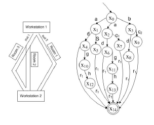
Figure 1: Manufacturing System (Left) and Plant (Right)

Consider a manufacturing system that consists of two workstations, three rooms and a robot as shown in Fig. 1 (Left). Initially, the robot is in workstation 1. By choosing rail 1 (event $a$), this robot nondeterministically goes to room 2 and room 3 and by choosing rail 2 (event $b$), it can go to room 1. If the robot is in room 2 and it hears the alarm (event $s$), it can go to the workstation 2 (event $r_{1}$). Or it can take a video (event $d$) when it is in room 2 and after that it has two choices : to go to workstation 2 (event $r_{1}$) or to receive the message from the host computer (event $g$). After the message has been received, the robot can active an energy-saving mode (event $h$) and then go to workstation 2 (event $r_{1}$). If the robot is in room 3, its behavior is similar to what it does in room 2 except that it can pick up a box from room 3 (event $c_{1}$) and then go to workstation 2 (event $r_{1}$). If it is in room 1, it also has two choices: to pick up a box from room 1 (event $c_{2}$) then go to workstation 2 (event $r_{1}$) or to take a video (event $d$) and after then go to workstation 2 (event $r_{1}$). In this model, we assume that the event $s$ describing that the robot hears the alarm is uncontrollable, the event $g$ describing that the robot receives a message from the host computer is uncontrollable and unobservable and all the rest events are controllable and observable.

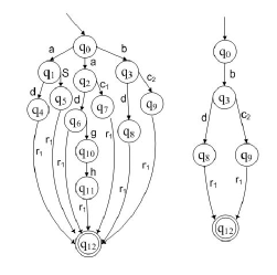
Figure 2: Specification (Left) and Supremal Simulation-Based Controllable and Strong Observable Subautomata (Right)

The automata model $G$ of the robot in manufacturing system is shown in Fig. 1 (Right). The specification $R$ is in Fig. 2 (Left) to restrict the behavior of $G$, which requires that the robot can go to the workstation 2 after hearing the alarm or go to workstation 2 after taking the video if it is in room 2. It can be seen that $L(G)=L(R)$. Thus, if we use language equivalence as a notion of behavioral equivalence, there is no need to control. However, as mentioned above, $G$ can exhibit some undesired behaviors, which motivates us to design a supervisor $S$ such that the controlled system $S/G$ is bisimilar to $R$. In [14], such a supervisor $S$ exists if and only if $R$ is simulation-based controllable and observable under partial observation. However, $R$ in this example is not simulation-based controllable and observable. In this paper, we want to calculate the supremal simulation-based controllable and strong observable subautomaton of $R$. By Algorithm 2, we obtain that $R$ is calculable for such kind of subautomaton. Next, we have $q_{2},q_{4}\in Q_{d}(Q\times X)$, $q_{1}\in Q_{d}^{\prime}(Q\times X)$ and $y_{1}=h_{3}(Q\times X)=\{(q_{0},x_{0}),(q_{3},x_{3}),\{q_{5},q_{7},q_{8},q_{9},q_{11}\}\times\{x_{4},x_{5},x_{6},x_{7},x_{8},x_{9},x_{12},x_{13}\},(q_{6},x_{4}),(q_{6},x_{6}),(q_{10},x_{10}),(q_{10},x_{11}),(q_{12},x_{14})\}$ in the first iteration. Further, $y_{2}=h_{3}(y_{1})=y_{1}$ and $(q_{0},x_{0})\in y_{2}$. Hence, the supremal simulation-based controllable and strong observable subautomata is achieved in Fig. 2 (Right).

VI CONCLUSIONS

By resorting to lattice theory, we proposed a computational approach to solve the supremal simulation-based controllable and strong observable subautomata, where both plant and specification are modeled as nondeterministic automata. The obtained solution provides a sufficient condition of the existence of the supremal simulation-based controllable and strong observable subautomta and an explicit algorithm to calculate such subautomta. Further, an example is generated to illustrate the proposed techniques.

References

• [1] R. Milner, Communication and Concurrency. Prentice Hall, New York, 1989.
• [2] J. Fernandez, ``An implementation of an efficient algorithem for bisimulation equivalence," Sci. Comput. Programming, vol. 13, pp. 219-236, 1990.
• [3] P. Tabuada and G. J. Pappas, ``Linear temporal logic control of discrete-time linear systems," IEEE Transactions on Automatic Control, vol. 51, pp. 1862-1877, December 2006.
• [4] V. Danos, J. Desharnais, F. Laviolette, ``Bisimulation and concongruence for probabilistic systems," Inform. Comput. Programming , vol. 204, pp. 503-523, 2006.
• [5] E. Haghverdi, P. Tabuada, and G. J. Pappas, ``Bisimulation relation for dynamical, control, and hybrid systems," Theoret. Comp. Sci., vol. 342, pp. 229-261, 2005.
• [6] J. Komenda and J. H. van Schuppen, ``Control of discrete-event systems with partial observations using coalgebra and coinduction," Discrete Event Dynamical Systems: Theory and Applications, vol. 15, pp. 257-315, 2005.
• [7] P. Tabuada and G. J. Pappas, ``Bisimilar control affine systems," Systems $\&$ Control Letters, vol. 52, pp. 49-58, 2004.
• [8] P. Tabuada, ``Controller synthesis for bisimulation equivalence," Systems $\&$ Control Letters, vol. 57, pp. 443-452, 2008.
• [9] C. G. Cassandtras and S. Lafortune, Introduction to Discrete Event Systems. Boston, MA: Kluwer, 1999.
• [10] Y. Sun, H. Lin, F. Liu, Ben M. Chen, ``Computation for Supremal Simulation-Based Controllable Subautomata," In Proceedings of 8th IEEE International Conference on Control and Automation, pp. 1450-1455, Xiamen, China, June 9-11, 2010.
• [11] R. Kumar and V. K. Garg, Modeling and Control of Logical Discrete Event Systems. Kluwer Academic Publishers, Boston, MA, 1995.
• [12] E. A. Emerson, `` Temporal and Modal Logic", In J. van leeuwen, editor, Handboook of Theoretical Computer Science: Formal Models and Semantics, North-Holland Pub. Co./MIT Press, volume B, pp. 995-1072.
• [13] C. Zhou, R. Kumar, and S. Jiang, ``Control of Nondeterministic Discrete Event Systems for Bisimulation Equivalence," IEEE Transactions on Automatic Control, vol. 51, pp. 754-765, 2006.
• [14] F. Liu, D. Qiu, and H. Lin, ``Bisimilarity control of nondeterministic discrete event systems," submitted for publication, 2010.
• [15] Paulo Tabuada, Verification and Control of Hybrid Systems, Springer, 2009.
• [16] R. Kumar and V. K. Garg, ``Extremal Solutions of Inequations over Lattices with Applications to Supervisory Control," Theoretical Computer Science, vol. 148, pp. 67-92, November 1995.
• [17] R. D. Brandt, V. K. Garg, R. Kumar, F. Lin, S. I. Marcus, and W. M. Wonham, ``Formulas for Calculating Supremal Controllable and Normal Sublanguages," Systems and Control Letters, vol. 15, pp. 111-117, August 1990.