Temperature-dependent spin resonance energy in iron pnictides and multiband $s\pm$ Eliashberg theory

Abstract

The phenomenology of iron-pnictides superconductors can be explained in the framework of a three bands s$\pm$ wave Eliashberg theory with only two free parameters plus a feedback effect i.e. the effect of the condensate on the antiferromagnetic spin fluctuactions responsible of the superconductivity in these compounds. I have examined the experimental data of four materials: $\mathrm{LaFeAsO_{1-x}F_{x}}$, $\mathrm{SmFeAsO_{1-x}F_{x}}$, $\mathrm{Ba_{1-x}K_{x}Fe_{2}As_{2}}$, and $\mathrm{Ba(Fe_{x}Co_{1-x})_{2}As_{2}}$ and I have found that it is possible to reproduce the experimental critical temperature and gap values in a moderate strong-coupling regime: $\lambda_{tot}\approx 1.7-2.0$.

The new class of Fe-based compounds Kamihara_La ; Ren_Sm ; Wang_Gd just as the cuprates Chubukov and the heavy fermions HF have all some similar caracteristics. For example the high values of rate $2\Delta/T_{c}$ or the presence of the pseudogap Chubukov ; HFAR ; Gonnelli_La . For all three class of material it is proposed the superconductivity to be mediated by antiferromagnetic spin fluctuactions Chubukov ; HFTH ; Mazin_PhysC_SI . The most obvious difference is that almost all the iron compounds present a multiband behavior while in HTCS and in heavy fermions this was detected only in some particular cases. The multi-band nature of Fe-based superconductors may give rise to a multi-gap scenario Tes that is indeed emerging from many different experimental data with evidence for rather high gap ratios, $\approx 2-3$ PhysC_Fe . In this regard neither a three-band BCS model Mazin_PhysC_SI ; Benfatto ; Kuchinskii nor a four-band Eliashberg model Ema with small values of the coupling constants and large boson energies are adequate: the former can only account for the gap ratio and $T_{c}$ but not for the exact experimental gap values and the latter provides a calculated critical temperature larger than the experimental one. The high experimental value of the larger gap suggests that high values of the coupling constants might be necessary to explain the experimental data within a three-band model Umma1 ; Umma2 : one has therefore to employ the Eliashberg theory for strong coupling superconductors Umma1 ; Umma2 . In my early works Umma1 ; Umma2 I found that a three-band Eliashberg model allows to reproduce various experimental data, this suggests that these compounds can represent a case of dominant negative interband-channel superconductivity ($s\pm$ wave symmetry) with small typical boson energies ($\approx 10$ meV) but too high values of the electron-boson coupling constants ($1.9\leq\lambda_{tot}\leq 5.9$). The way for solve this problem is suggested by experimental measurement of Inosov and coworkers Inosov : they find that the temperature evolution of the spin resonance energy follows the superconducting energy gap and this should indicate a feedback effect Chubukov ; FBB ; FB of the condensate on the spin fluctuactions. I assume that this is the starting point of my argumentation. The procedure is as follows: first of all I choose the experimental low temperature spin resonance as representative boson energy and I fix the two remaining free parameters to reproduce the exact experimental gap values. then, with the same parameters, I calculate the critical temperature $T^{*}_{c}$. I find always $T^{*}_{c}\gg T^{exp}_{c}$ where $T^{exp}_{c}$ is the experimental critical temperature. In the successive step I use the same input parameters utilized before except for the electron-boson spectral functions that have an energy peak with the same temperature dependence of the superconductive gap. Of course at $T=T^{*}_{c}$ the energy peak is equal to zero while at $T=0$ K the new spectral functions are equal to old ones. In this way, taking into account the feedback effect of the condensate Chubukov ; FBB ; FB on the antiferromagnetic spin fluctuactions I could explain the experimental data (the gap values and the critical temperature) in a model which has only two free parameters in a moderate strong coupling regime ($\lambda_{tot}\approx 1.7-2$).

I choose four representative cases (three hole type and one electron type): $\mathrm{LaFeAsO_{1-x}F_{x}}$, $\mathrm{SmFeAsO_{1-x}F_{x}}$, $\mathrm{Ba_{1-x}K_{x}Fe_{2}As_{2}}$, and $\mathrm{Ba(Fe_{x}Co_{1-x})_{2}As_{2}}$. The electronic structure of the compounds hole type can be approximately described by a three-band model Mazin_PhysC_SI with two hole bands (indicated in the following as bands 1 and 2) and one equivalent electron band (3) Umma1 ; Umma2 while for one electron type with one hole band (indicated in the following as band 1) and two equivalent electron bands (2 and 3) Tortello2010 . In the hole type case the $s$-wave order parameters of the hole bands $\Delta_{1}$ and $\Delta_{2}$ have opposite sign compared to electron band one, $\Delta_{3}$ Mazin_spm while, in the electron type case, $\Delta_{1}$ has opposite sign compared to two electron bands ones, $\Delta_{2}$ and $\Delta_{3}$ Tortello2010 . In such systems, intraband coupling could be provided by phonons (ph), and interband coupling by antiferromagnetic spin fluctuations (sf) Mazin_spm . I summarize the experimental data relative to the four considered cases:

1) the compound $\mathrm{LaFeAsO_{0.9}F_{0.1}}$ (LaFeAsOF)with $T^{A}_{c}=28.6$ K where point-contact spectroscopy measurements gave $\Delta_{1}(0)\approx 8.0$ meV and $\Delta_{2}(0)\approx 2.8$ meV Gonnelli_La ;

2) $\mathrm{Ba_{0.6}K_{0.4}Fe_{2}As_{2}}$ (BaKFeAs) with $T_{c}=37$ K where ARPES measurements gave $\Delta_{1}(0)=12.1\pm 1.5$ meV, $\Delta_{2}(0)=5.2\pm 1.0$ meV and $\Delta_{3}(0)=12.8\pm 1.4$ meV Ding_ARPES_BaKFeAs ;

3) the compound $\mathrm{SmFeAsO_{0.8}F_{0.2}}$ (SmFeAsOF) with $T^{A}_{c}=52$ ($T^{bulk}_{c}=53$ K) K where, according to point-contact spectroscopy measurements, $\Delta_{1}(0)=18\pm 3$ meV and $\Delta_{2}(0)=6.2\pm 0.5$ meV Daghero_Sm ;

4) the compound $\mathrm{Ba(Fe_{x}Co_{1-x})_{2}As_{2}}$ (BaFeCoAs) with $T^{A}_{c}=22.6$ K ($T^{bulk}_{c}=24.5$ K) where, according to point-contact spectroscopy measurements, $\Delta_{1}(0)=4.1\pm 0.4$ meV and $\Delta_{2}(0)=9.2\pm 1.0$ meV Tortello2010 .

$T^{A}_{c}$ is the critical temperature obtained by Andreev reflection measurements and $T^{bulk}_{c}$ is the critical temperature extracted by transport measurements. Note that only in the case of ARPES the gaps are associated to the relevant band since point-contact spectroscopy measurements generally gives only two gaps, the larger one has been arbitrarily indicated as $\Delta_{1}$ supposing that $\Delta_{1}\sim|\Delta_{3}|$.

	$\lambda_{tot}$	$\lambda^{old}_{tot}$	$\lambda_{12/21}$	$\lambda_{13/31}$	$\lambda_{23/32}$	$\Omega_{0}$ (meV)
	1.87		0.76/0.85	1.21/5.44	0.00/0.00	9.04
BaFeCoAs	2.83	1.93	0.91/1.02	2.08/9.35	0.00/0.00	9.04
	1.75		0.00/0.00	2.11/1.91	0.40/0.21	11.44
LaFeAsOF	2.38	2.53	0.00/0.00	2.93/2.66	0.46/0.24	11.44
	2.04		0.00/0.00	2.27/2.27	0.56/0.28	14.80
BaKFeAs	2.84	3.87	0.00/0.00	3.21/3.21	0.67/0.34	14.80
	1.72		0.00/0.00	1.55/3.88	0.42/0.84	20.80
SmFeAsOF	2.39	5.90	0.00/0.00	2.23/5.58	0.49/0.98	20.80

Table 1: The values of $\Omega_{0}$ and $\lambda_{ij}$, that allow reproducing the experimental gap values, are shown. $\lambda_{tot}$ is compared with $\lambda^{old}_{tot}$ that is the value determined in the previous works Umma1 ; Umma2 ; Tortello2010 . In the first arrows the sf spectral functions used have usual shape while in the second ones have Lorentzian shape.

	$\Delta_{1}(meV)$	$\Delta_{2}(meV)$	$\Delta_{3}(meV)$	$T_{c}(K)$	$T^{*}_{c}(K)$
	6.63	-4.07	-9.18	26.07	33.00
BaFeCoAs	7.02	-4.12	-9.18	23.73	28.95
	8.01	2.82	-7.75	29.37	37.22
LaFeAsOF	8.01	2.77	-7.71	26.86	31.81
	12.04	5.20	-12.00	43.66	55.26
BaKFeAs	12.04	5.24	-11.91	38.33	46.18
	14.86	6.15	-18.11	58.53	74.13
SmFeAsOF	15.51	6.15	-18.00	52.80	63.82

Table 2: The calculated values of the gaps and of the two critical temperature with and without feedback effect. In the first arrows the sf spectral functions used have usual shape while in the second ones have Lorentzian shape.

To obtain the gaps and the critical temperature within the s$\pm$ wave, three-band Eliashberg equations Eliashberg one has to solve six coupled equations for the gaps $\Delta_{i}(i\omega_{n})$ and the renormalization functions $Z_{i}(i\omega_{n})$, where $i$ is a band index (that ranges between $1$ and $3$) and $\omega_{n}$ are the Matsubara frequencies. If one neglects for simplicity the effect of magnetic and non-magnetic impurities, the imaginary-axis equations Umma1 ; Umma2 are:

$$\omega_{n}Z_{i}(i\omega_{n})=\omega_{n}+\pi T\sum_{m,j}\Lambda^{Z}_{ij}(i\omega_{n},i\omega_{m})N^{Z}_{j}(i\omega_{m})$$ (1)

$$Z_{i}(i\omega_{n})\Delta_{i}(i\omega_{n}) = \pi T\sum_{m,j}[\Lambda^{\Delta}_{ij}(i\omega_{n},i\omega_{m})$$

$$-\mu^{*}_{ij}(\omega_{c})]\Theta(\omega_{c}-|\omega_{m}|)N^{\Delta}_{j}(i\omega_{m})\vspace{5mm}$$

where $\Lambda^{Z}_{ij}(i\omega_{n},i\omega_{m})=\Lambda^{ph}_{ij}(i\omega_{n},i\omega_{m})+\Lambda^{sf}_{ij}(i\omega_{n},i\omega_{m})$, $\Lambda^{\Delta}_{ij}(i\omega_{n},i\omega_{m})=\Lambda^{ph}_{ij}(i\omega_{n},i\omega_{m})-\Lambda^{sf}_{ij}(i\omega_{n},i\omega_{m})$. $\Theta$ is the Heaviside function and $\omega_{c}$ is a cutoff energy. In particular, $\Lambda^{ph,sf}_{ij}(i\omega_{n},i\omega_{m})=2\int_{0}^{+\infty}d\Omega\Omega\alpha^{2}_{ij}F^{ph,sf}(\Omega)/[(\omega_{n}-\omega_{m})^{2}+\Omega^{2}]$. $\mu^{*}_{ij}(\omega_{\rm c})$ are the elements of the $3\times 3$ Coulomb pseudopotential matrix. Finally, $N^{\Delta}_{j}(i\omega_{m})=\Delta_{j}(i\omega_{m})/{\sqrt{\omega^{2}_{m}+\Delta^{2}_{j}(i\omega_{m})}}$ and $N^{Z}_{j}(i\omega_{m})=\omega_{m}/{\sqrt{\omega^{2}_{m}+\Delta^{2}_{j}(i\omega_{m})}}$. The electron-boson coupling constants are defined as $\lambda^{ph,sf}_{ij}=2\int_{0}^{+\infty}d\Omega\frac{\alpha^{2}_{ij}F^{ph,sf}(\Omega)}{\Omega}$.

The solution of eqs. 1 and Temperature-dependent spin resonance energy in iron pnictides and multiband $s\pm$ Eliashberg theory requires a huge number of input parameters (18 functions and 9 constants); however, some of these parameters are related one to another, some can be extracted from experiments and some can be fixed by suitable approximations. As shown in Ref. Mazin_spm , in the case of pnictides we can assume that: i) the total electron-phonon coupling constant is small Boeri2 ; ii) phonons mainly provide intraband coupling; iii) spin fluctuations mainly provide interband coupling. To account for these assumptions in the simplest way, I will take: $\lambda^{ph}_{ii}=\lambda^{ph}_{ij}=0.$ (upper limit of the phonon coupling Boeri2 $\approx 0.35$), $\lambda^{sf}_{ii}=0$ (only interband sf coupling) and $\mu^{*}_{ii}(\omega_{\rm c})=\mu^{*}_{ij}(\omega_{\rm c})=0$ Umma1 . Within these approximations, the electron-boson coupling-constant matrix $\lambda_{ij}$ becomes: Mazin_PhysC_SI ; Umma1 ; Tortello2010 :

$$\vspace{2mm}\lambda_{ij}=\left(\begin{array}[]{ccc}0&\lambda_{12}&\lambda_{13}\\ \lambda_{21}=\lambda_{12}\nu_{12}&0&\lambda_{23}\\ \lambda_{31}=\lambda_{13}\nu_{13}&\lambda_{32}=\lambda_{23}\nu_{23}&0\\ \end{array}\right)$$ (3)

where $\nu_{ij}=N_{i}(0)/N_{j}(0)$ and $N_{i}(0)$ is the normal density of states at the Fermi level for the $i$-th band. In the hole case it is $\lambda_{21}=\lambda_{12}=0$ while in the electron case $\lambda_{23}=\lambda_{32}=0$. In the numerical simulations I used the standard form for the antiferromagnetic spin fluctuaction dolghi : $\alpha^{2}_{ij}F^{sp}(\Omega)=B_{ij}\Omega\cdot\Omega_{ij}\cdot\Theta(\Omega_{max}-\Omega)/(\Omega^{2}+\Omega^{2}_{ij})$ where $B_{ij}$ are the normalization constants necessary to obtain the proper values of $\lambda_{ij}$ while $\Omega_{ij}$ are the peak energies. In all the calculations I always set $\Omega_{ij}=\Omega_{0}$. The maximum sf energy is $\Omega_{max}=10\Omega_{0}$, the cut-off energy is $\omega_{c}=30\Omega_{0}$ and the maximum quasiparticle energy is $\omega_{max}=40\Omega_{0}$. As typical sf energy $\Omega_{0}$ I use the spin resonance energy that have been measured and I assume correct for all compounds examined the relation $\Omega_{0}=(2/5)T_{c}$ available in literature Paglione . Bandstructure calculations provide information about the factors $\nu_{ij}$ that enter in the definition of $\lambda_{ij}$ (eq. 3). In the case of $\mathrm{LaFeAsO_{0.9}F_{0.1}}$ I know that $\nu_{13}=0.91$ and $\nu_{23}=0.53$ Mazin4 , in $\mathrm{Ba_{0.6}K_{0.4}Fe_{2}As_{2}}$ $\nu_{13}=1$ and $\nu_{23}=2$ Mazin_PhysC_SI , in $\mathrm{SmFeAsO_{0.8}F_{0.2}}$ $\nu_{13}=0.4$ and $\nu_{23}=0.5$ Mazin4 and in $\mathrm{Ba(Fe_{x}Co_{1-x})_{2}As_{2}}$ $\nu_{12}=1.12$ and $\nu_{13}=4.50$ Mazin4 .

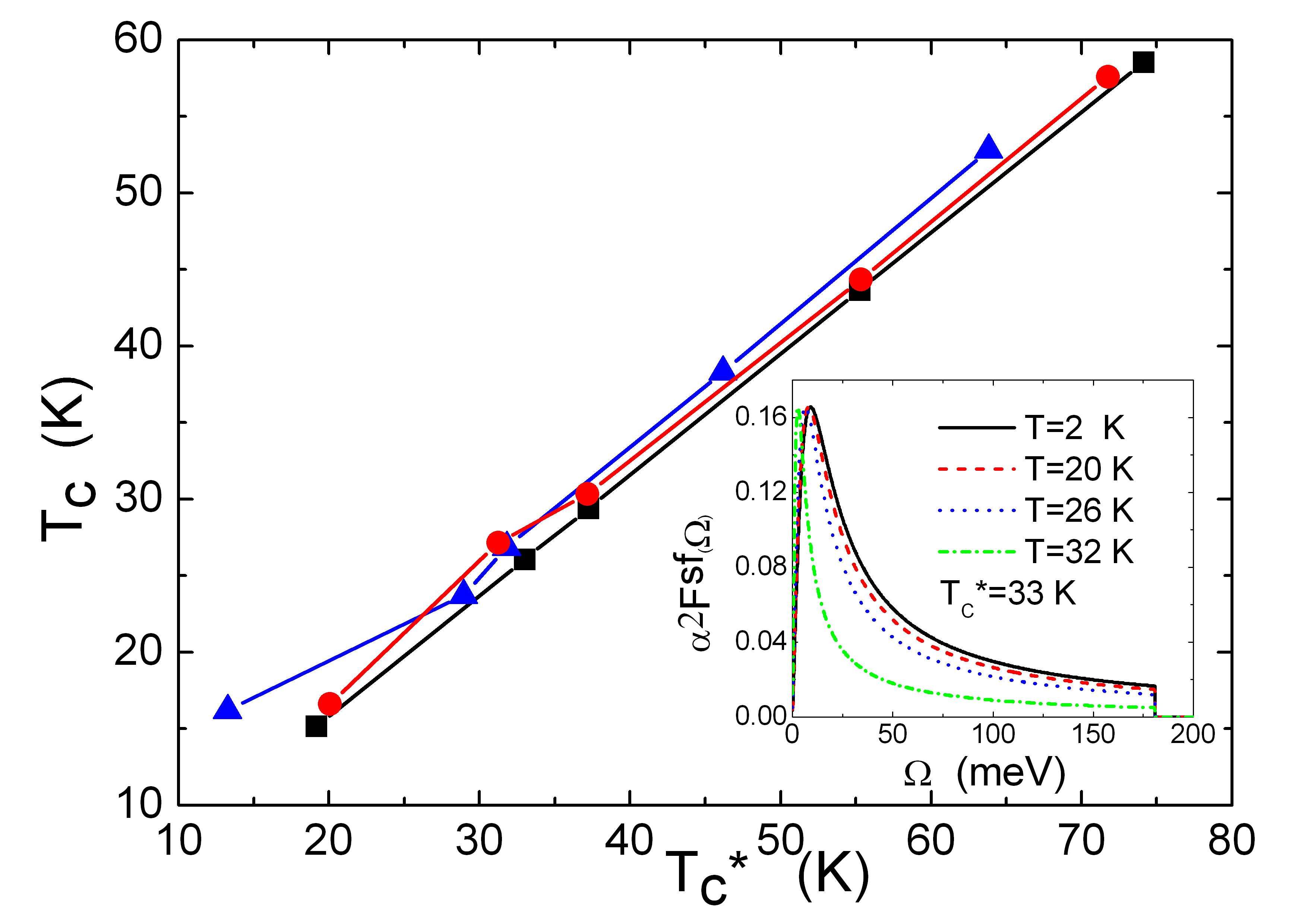
Figure 1: (Color online) The calculated critical temperature $T_{c}$ with feedback effect versus standard critical temperature $T^{*}_{c}$ in three different situations: only interband sf coupling with standard spectral functions (black squares), interband sf coupling with standard spectral functions and small intraband ph coupling (red circles) and only interband sf coupling with Lorentz spectral functions (dark blue triangles). In the bottom right insert the sf spectral function, for the $\mathrm{Ba(Fe_{x}Co_{1-x})_{2}As_{2}}$, at different temperatures ($T<T_{c}^{*}$) with the feedback effect.

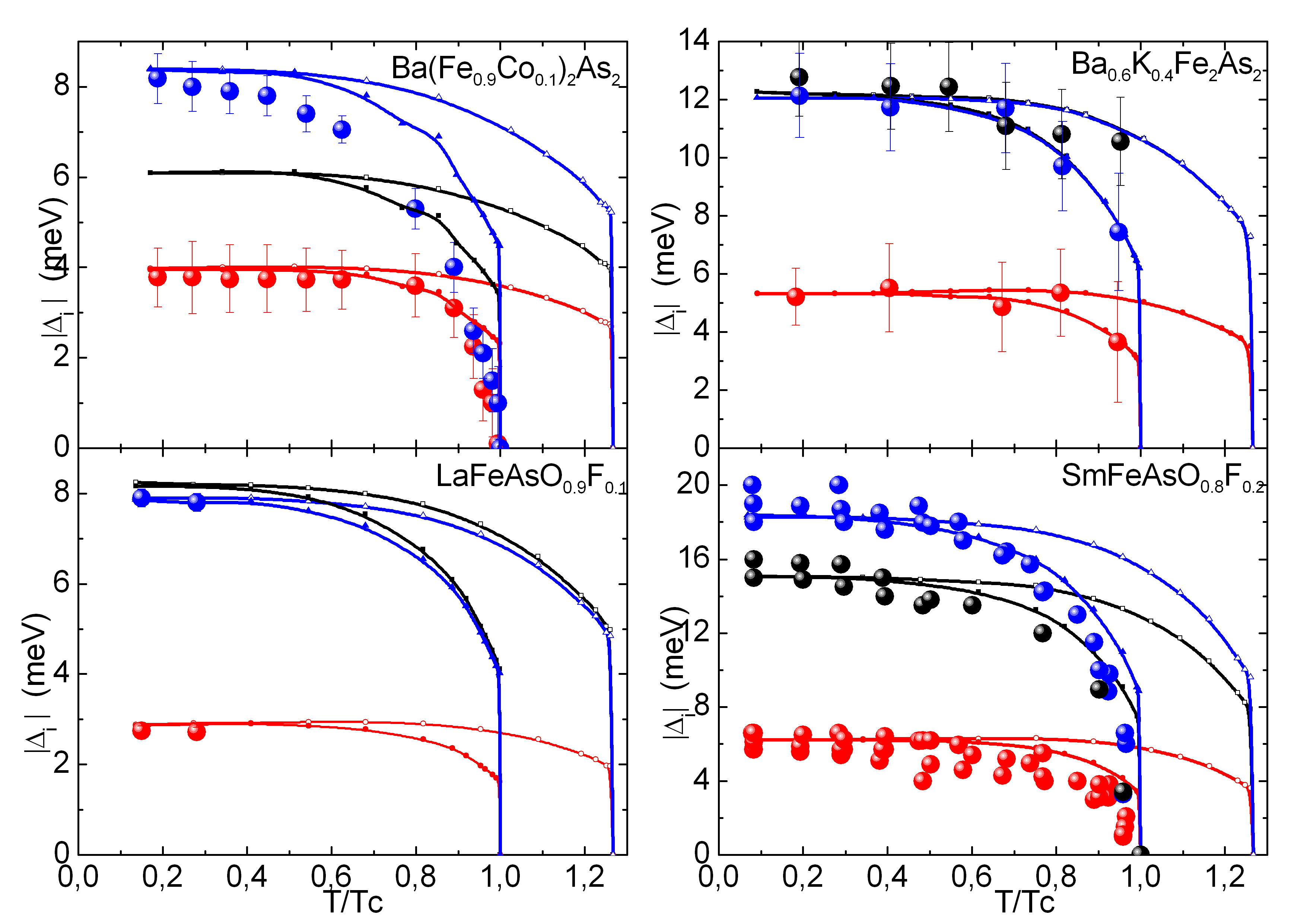
Figure 2: (Color online) The calculated temperature dependence of $|\Delta_{i}|$ from the solution of real axis Eliashberg equations in the standard case (open symbol) and when the feedback effect is present (solid symbol): $|\Delta_{1}|$ black squares, $|\Delta_{2}|$ red circles and $|\Delta_{3}|$ dark blue triangles. The experimental data Gonnelli_La ; Ding_ARPES_BaKFeAs ; Daghero_Sm ; Tortello2010 are shown as big solid circles.

I initially solve the imaginary-axis Eliashberg equations (eqs. 1 and Temperature-dependent spin resonance energy in iron pnictides and multiband $s\pm$ Eliashberg theory) to calculate the low-temperature value of the gaps (which are actually obtained by analytical continuation to the real axis by using the technique of the Padé approximants) and so I fix the two free parameters of the model: $\lambda_{13}$ and $\lambda_{23}$ ($\lambda_{12}$). By properly selecting the values of $\lambda_{13}$ and $\lambda_{23}$ ($\lambda_{12}$) it is relatively easy to obtain the experimental values of the gaps with reasonable values of $\lambda_{tot}=\frac{\sum_{ij}N_{i}(0)\lambda_{ij}}{\sum_{ij}N_{i}(0)}$ (between 1.72 and 2.04). However, in all the materials examined, the high $2\Delta_{1,3}/k_{B}T_{c}$ ratio (of the order of 8-9) makes it possible to reproduce also the values of the large gap(s) only if the calculated critical temperature $T^{*}_{c}$ is considerably higher than the experimental one. For solving this problem also present in the HTCS, I assume that exist a effect of feedback Chubukov ; FBB ; FB of the condensate and, in a phenomenological way, I introduce in the Eliashberg equation a temperature dependence of the representative boson energy $\Omega_{0}(T)=\Omega_{0}tanh(1.76\sqrt{T^{*}_{c}/T-1})$ that reproduces both the approximate gap temperature dependence in the strong coupling case FB and the experimental spin resonance one Inosov . The primary effect of this assumption is lowering the critical temperature leaving unchanged the gap values at $T<<T^{*}_{c}$ because the critical temperature is roughly proportional to electron boson coupling constant and to representative boson energy $\Omega_{0}(T)$ of the material: in this case $\Omega_{0}(T)$ decreases and so $T_{c}$. For a completely consistent procedure it should used $\Omega_{0}(T)=\Omega_{0}\eta(T)$ where $\eta(T)$ is the temperature dependence part of the superfluid density $\rho(T)=\rho(0)\eta(T)$ and $\rho(0)$ is the superfluid density at $T=0$ K. $\eta(T)$ is a function of $\Delta_{i}(i\omega_{n})$ and so, in this way, the numerical solution of Eliashberg equations become remarkably more complex and time consuming. I am conscious that the temperature dependence of $\Omega_{0}(T)$ is added ad hoc and it is not obtained self-consistent but this is an attempt in order to determine if the chosen path can lead to interesting results. What is important is that this mechanism of feedback can justify the experimental values for the gaps, their dependence on temperature and the critical temperature with a model that has only two free parameters. Moreover, the parameters determined are reasonable and $\lambda_{tot}$ is very similar for all four materials examined and in agreement with the values proposed by other authors dolghi . I solve the Eliashberg equations in three different situations: 1) only sf interband coupling is present and the sf spectral functions have usual shape; 2) sf interband coupling with a small ph intraband contribution are present and sf spectral functions have usual shape; 3) only sf interband coupling is present and the sf spectral functions have Lorentz shape. In the first case the coupling constant $\lambda_{tot}$ is in the range 1.72-2.04. The results are almost independent from $\Omega_{max}$ because, for example in the case of $BaFeCoAs$, multiplying $\Omega_{max}$ by a factor two, I obtain the same values of the gaps and $T_{c}$ with $\lambda_{tot}=1.68$ i.e. with a reduction of 0.18 which is very small. The agreement with the experimental critical temperature is good. It is noticeable the small variation of the total coupling in the four compounds considered. In the second case there is also a intraband phonon contribution, equal in any band and in any compound for simplicity, with $\lambda^{ph}_{ii}=0.35$ and $\Omega^{ph}_{0}=18$ meV that are the upper limits for the ph coupling constants and the representative ph energies Boeri2 . The ph spectral functions have Lorentzian shape Umma1 with the peaks at the same energy: $\Omega_{ij}=\Omega^{ph}_{0}$and with half width always equal to 2 meV ( $\omega_{c}=12\Omega^{ph}_{0}$). $\lambda_{tot}$ and $T_{c}$ are practically the same as the previous case. This last fact indicate that the effect of intraband phonon contribution is negligible. In the third case (Lorentz shape of sf spectral functions) the agreement with the experimental critical temperatures is very good in all compounds but the total coupling is more large ($2.38\leq\lambda_{tot}\leq 2.84$). In Fig. 1 it is possible to see the linear relation between $T_{c}$ and $T^{*}_{c}$ in all three examined cases. In table 1 are shown the inputs parameters of the Eliashberg equations in the first and third case examined for the four compounds. In table 2 are shown the calculated values of the gaps and the critical temperatures $T_{c}$ and $T^{*}_{c}$ obtained by numerical solution of Eliashberg equations. Once the values of the low-temperature gaps were obtained, I calculated their temperature dependence by directly solving the three-band Eliashberg equations in the real-axis formulation instead of using the analytical continuation to the real axis of the imaginary-axis solution. Of course, the results of the two procedures are virtually identical at low temperature. In all cases, their behavior is rather unusual and completely different from the BCS one, since the gaps slightly decrease with increasing temperature until they suddenly drop close to $T_{c}$. This arises from a complex non-linear dependence of the $\Delta$ vs. $T$ curves on $\lambda_{ij}$ and is possible only in a strong-coupling regime UmmaT . Curiously in all four compounds the rate $T^{*}_{c}/T_{c}$ is $1.27$. As it is shown in Fig. 2 the calculated temperature dependencies of $|\Delta_{i}|$ are compared with the experimental data and the agreement is very good (in the case of $\mathrm{Ba(Fe_{x}Co_{1-x})_{2}As_{2}}$ I compare the temperature dependence of the gaps with these particular experimental valuesTortello2010 : $\Delta_{1}=3.8$ meV and $\Delta_{2}=8.2$ meV and I find $\lambda_{12}=0.77$, $\lambda_{13}=1.05$ and $T_{c}=23.43$ K). In conclusion, I have shown that a simple Eliashberg three-band model, with antiferromagnetic spin fluctuactions-electrons coupling, in moderate strong-coupling regime with only two free parameters and a feedback effect can reproduce, in a quantitative way, the experimental critical temperature and the amplitude of the energy gaps.

I thank R.S. Gonnelli, E. Cappelluti, Lara Benfatto and Sara Galasso for the useful and clarifying discussions.

References

- (1) Y. Kamihara et al., J. Am. Chem. Soc. 130, 3296-3297 (2008).
- (2) Ren Zhi-An et al., Chin. Phys. Lett.25, 2215 (2008).
- (3) Cao Wanget al., Europhys. Lett. 83, 67006 (2008).
- (4) A.V. Chubukov, D. Pines, and J. Schmalian, A Spin Fluctuation Model for d-Wave Superconductivity; D. Manske, I. Eremin, and K.H. Bennemann, Electronic Theory for Superconductivity in high- Cuprates and , K.H. Bennemann and J.B. Ketterson Editors, Volume II. Superconductivity: Novel Superconductors, Springer-Verlag Berlin Heidelberg (2008).
- (5) P. Thalmeier et al., Superconductivity in Heavy Fermion Compounds, A. Narlikar (Ed.) Frontiers in Superconducting Materials, Springer Verlag, Berlin, (2005).
- (6) W.K. Park and L.H. Greene, J. Phys.: Condens. Matter 21 103203 (2009).
- (7) R.S. Gonnelli et al., Phys. Rev. B 79, 184526 (2009).
- (8) J. Chang, I. Eremin, P. Thalmeier, P. Fulde, Phys. Rev. B 75, 024503 (2007); I. Eremin, G. Zwicknagl, P. Thalmeier, P. Fulde, Phys. Rev. Lett. 101, 187001 (2008).
- (9) I.I. Mazin and J. Schmalian, Physica C 469, 614 (2009).
- (10) V. Cvetkovic and Z. Tesanovic, Europhys. Lett. 85, 37002, (2009);
- (11) Physica C 469, (2009), Special Issue on Pnictides.
- (12) L. Benfatto, M. Capone, S. Caprara, C. Castellani, C. DiCastro, Phys. Rev. B 78, 140502(R) (2008).
- (13) E. Z. Kuchinskii, M. V. Sadovskii, JETP Letters, 89, 156 (2009).
- (14) L. Benfatto, E. Cappelluti and C. Castellani, Phys. Rev. B 80, 214522 (2009).
- (15) G.A. Ummarino, M. Tortello, D. Daghero, R.S. Gonnelli, Phys. Rev. B 80, 172503 (2009).
- (16) G.A. Ummarino, M. Tortello, D. Daghero, R.S. Gonnelli, to be published in J. Supercond. Nov. Magn.
- (17) D.S. Inosov et al., Nature Physics 6, 178 (2010).
- (18) Ar. Abanov, A. V. Chubukov, and J. Schmalian, Journal of Electron Spectroscopy and Related Phenomena 117-118, 129 (2001).
- (19) A. Akbari, I. Eremin, P. Thalmeier, and P. Fulde, Phys. Rev. B 80, 100504 (2009) M.M. Korshunov and I. Eremin, Phys. Rev. B 78, 140509 (2008); T.A. Maier and D.J. Scalapino, Phys. Rev. B 78, 020514 (2008).
- (20) I.I. Mazin, D.J. Singh, M.D. Johannes, M.H. Du, Phys. Rev. Lett. 101, 057003 (2008).
- (21) P. Popovich et al., Phys. Rev. Lett,105, 027003 (2010).
- (22) G.M. Eliashberg, Sov. Phys. JETP 11, 696 (1960).
- (23) L. Boeri, M. Calandra, I.I. Mazin, O.V. Dolgov, F. Mauri, Phys. Rev. B 82, 020506 (2010).
- (24) H. Ding et al., Europhys. Lett. 83, 47001 (2008).
- (25) D. Daghero et al., Phys. Rev. B 80, 060502(R) (2009); R.S. Gonnelli et al., Physica C 469, 512 (2009).
- (26) M. Tortello et al., Phys. Rev. Lett,105, 237002 (2010).
- (27) J. Paglione and R.L. Greene, Nature Physics 6, 645 (2010).
- (28) I.I. Mazin, private communication.
- (29) G.A.Ummarino and R.S. Gonnelli, Physica C 328, 189 (1999).