Approximating travelling waves by equilibria of non local equations

Abstract

We consider an evolution equation of parabolic type in $\mathbb{R}$ having a travelling wave solution. We perform an appropriate change of variables which transforms the equation into a non local evolution one having a travelling wave solution with zero speed of propagation with exactly the same profile as the original one. We analyze the relation of the new equation with the original one in the entire real line. We also analyze the behavior of the non local problem in a bounded interval with appropriate boundary conditions and show that it has a unique stationary solution which is asymptotically stable for large enough intervals and that converges to the travelling wave as the interval approaches the entire real line. This procedure allows to compute simultaneously the travelling wave profile and its propagation speed avoiding moving meshes, as we illustrate with several numerical examples.

1 Introduction

We address the problem of the analysis and effective computation of travelling wave solutions emerging from parabolic semilinear equations on the real line:

$$\left\{\begin{array}[]{l}u_{t}(x,t)=\displaystyle u_{xx}(x,t)+f(u(x,t)),\qquad-\infty<x<+\infty,\quad t>0,\\[5.0pt] u(x,0)=u_{0}(x).\end{array}\right.$$ (1)

We assume that $f\in C^{1}$ with $f(0)=f(1)=0$, so that $u=0$ and $u=1$ are stationary solutions of (1). Under these assumptions, if the initial data $u_{0}$ is piecewise continuous and $0\leq u_{0}\leq 1$, there exists a unique bounded classical solution $u(x,t)$ defined for all $t>0$ and, due to the maximum principle, $0\leq u(x,t)\leq 1$ for all $x,t$.

A travelling wave is a solution of the type $u(x,t)=\Phi(x-ct)$ where the function $\Phi$ is the profile of the travelling wave and $c$ is the speed of propagation of the wave. For instance, if $c>0$ (resp. $c<0$) the solution will consist of the profile $x\to\Phi(x)$ travelling in space to the right (resp. left) with speed $|c|$. Proofs of the existence of this kind of solutions can be found in [1, 13, 19] among others.

The asymptotic profile $\Phi$, when it exists, will have finite limits at $\pm\infty$, either $\Phi(-\infty)=0$, $\Phi(\infty)=1$ or $\Phi(-\infty)=1$, $\Phi(\infty)=0$. In the first case $\Phi$ will be a solution to

$$\left\{\begin{array}[]{l}\Phi^{\prime\prime}(\xi)+c\Phi^{\prime}(\xi)+f(\Phi(\xi))=0,\qquad-\infty<\xi<+\infty,\\[5.0pt] 0\leq\Phi\leq 1,\qquad\Phi(-\infty)=0,\ \Phi(+\infty)=1,\qquad\Phi^{\prime}>0,\end{array}\right.$$ (2)

that is called a $[0,1]$-wave front. The monotonicity condition on the profile $\Phi$ is not a restriction but rather an intrinsic property of the travelling wave profiles, as it is shown in [13, Lemma 2.1.].

Note also that, by simply making the change of coordinates $\xi\to-\xi$, to every pair $(\Phi,c)$ with $\Phi$ a monotone increasing $[0,1]$-wave front corresponds a monotone decreasing $[1,0]$-wave front with propagation speed $-c$. Thus, all what follows applies to monotone decreasing solutions as well.

These profiles are well known to have the property of attracting, as $t\to\infty$, the dynamics of a significant class of solutions of the Cauchy problem (1), see for instance Theorem 1 below (from [13]). In [13] it is proven that if $f$ is of bistable type satisfying

$$\left\{\begin{array}[]{l}f(0)=f(1)=0,\\ f^{\prime}(0)<0,f^{\prime}(1)<0,\\ \exists\alpha\in(0,1),\hbox{ s.t }f(u)<0,\quad\mbox{for }\ u\in(0,\alpha),\quad f(u)>0,\quad\mbox{for }\ u\in(\alpha,1).\end{array}\right.$$ (3)

then, for a certain set of initial data $u_{0}$, the solution $u(x,t)$ of (1) evolves into a travelling wave $\Phi(x-x_{0}-ct)$, for a certain $x_{0}\in\mathbb{R}$ depending on the initial datum $u_{0}$, i.e.,

$$|u(x,t)-\Phi(x-x_{0}-ct)|\to 0,\qquad\mbox{as }\ t\to\infty.$$ (4)

Further, the convergence in (4) is shown to be uniform in $x$ and exponentially fast in $t$.

From the numerical point of view, one of the main difficulties in the approximation of these asymptotic solutions $\Phi$ and their propagation speed $c$ is the need of setting a finite computational domain. While the solution $u$ evolves into $\Phi$, it also moves left or right at velocity $c$ and it eventually leaves the chosen finite computational domain. A natural approach is then to perform the change of variables $u(x,t)=v(x-ct,t)$, so that the resulting initial value problem for $v$ converges to a stationary solution, i.e, $v_{t}\to 0$ as $t\to\infty$. However, in general, the value of $c$ is not known a priori.

The issue of having a priori characterizations of the velocity of propagation $c$ then plays an important role from a computational viewpoint. It has been addressed in a number of articles. For instance, in [28] explicit mini-max representations for the speed of propagation $c$ are provided. Unfortunately, the expressions in [28] are difficult to handle in practice for the effective computation of $c$ and $\Phi$.

In the present paper, we follow and further develop the approach introduced in [5], where a new unknown $\gamma(t)$ is added to the problem, to perform the change of variables

$$u(x,t)=v(x-\gamma(t),t).$$ (5)

Then, $v$ satisfies the equation

$$v_{t}(x,t)=v_{xx}(x,t)+\gamma^{\prime}(t)v_{x}(x,t)+f(v).$$

Our goal is to determine $\gamma=\gamma(t)$ a priori so as to ensure that, as time evolves, it converges to the asymptotic speed $c$ of the travelling wave. Of course, in order to compensate for the additional unknown $\gamma$, one has to add a so called “phase condition”, that is, an additional equation linking $v$ and $\lambda:=\gamma^{\prime}$. Two different possibilities were proposed in [5]. One of them consists on minimizing the $L^{2}$-distance of the solution $v$ to a given template function $\hat{v}(x)$, which must satisfy $\hat{v}-\Phi\in H^{1}(\mathbb{R})$. This approach leads to a Partial Differential Algebraic Equation of the form

$$\left\{\begin{array}[]{l}v_{t}=\displaystyle v_{xx}+\lambda v_{x}+f(v),\quad-\infty<x<\infty,\quad t>0,\\[10.00002pt] 0=\langle\hat{v}^{\prime},v-\hat{v}\rangle,\\[10.00002pt] v(x,0)=u_{0}(x),\end{array}\right.$$ (6)

where $\langle\cdot,\cdot\rangle$ denotes the inner product in $L^{2}(\mathbb{R})$. This system is locally (in time) equivalent to the original one (1), provided that the implicit function theorem can be applied to the equation

$$\Phi(\gamma,t):=\langle\hat{v}^{\prime},u(\cdot+\gamma(t))-\hat{v}\rangle=0,$$

to obtain $\gamma(t)$ and $v(x,t)=u(x+\gamma(t),t)$, once $u$ is given, see [5, Theorem 2.9]. The approximation properties of (6) and its numerical discretizations have been studied in detail in [25, 26, 27]. This approach is useful as long as a suitable template mapping $\hat{v}$, close enough to $\Phi$, is available and the initial data $u_{0}$ belongs to $\Phi+H^{1}(\mathbb{R})$, too. From the computational point of view, the semidiscretization in space of (6) leads to a Partial Differential Algebraic Equation of index 2. This means that it is necessary to differentiate twice the algebraic constraint in order to eliminate it and get the underlying Partial Differential Equation, see for instance [17, Chap. VII].

A more global approach, also proposed in [5], is obtained by minimizing $\|v_{t}\|_{2}$. This yields the augmented system

$$\left\{\begin{array}[]{l}v_{t}=\displaystyle v_{xx}+\lambda v_{x}+f(v),\quad-\infty<x<\infty,\quad t>0,\\[10.00002pt] 0=\lambda\langle v_{x},v_{x}\rangle+\langle f(v),v_{x}\rangle,\\[10.00002pt] v(x,0)=u_{0}(x),\end{array}\right.$$ (7)

which is a Partial Differential Algebraic Equation of index 1. Assuming that the products above are well defined and $\|v_{x}(\cdot,t)\|_{2}\neq 0$, $t>0$, the phase condition

$$0=\lambda\langle v_{x},v_{x}\rangle+\langle f(v),v_{x}\rangle$$

yields directly

$$\gamma(t)=-\int_{0}^{t}\frac{\langle f(u(\cdot,s)),u_{x}(\cdot,s)\rangle}{\langle u_{x}(\cdot,s),u_{x}(\cdot,s)\rangle}\,ds=-\int_{0}^{t}\frac{\langle f(v(\cdot,s)),v_{x}(\cdot,s)\rangle}{\langle v_{x}(\cdot,s),v_{x}(\cdot,s)\rangle}\,ds,$$ (8)

and one gets the following nonlocal semilinear equation

$$\left\{\begin{array}[]{l}v_{t}=\displaystyle v_{xx}-\frac{\langle f(v),v_{x}\rangle}{\langle v_{x},v_{x}\rangle}\,v_{x}+f(v),\quad-\infty<x<\infty,\quad t>0,\\[10.00002pt] v(x,0)=u_{0}(x).\end{array}\right.$$ (9)

Definition (8) is in fact quite natural if we notice that, after multiplicating by $\Phi^{\prime}$ in (2) and integrating along the real line, we obtain

$$c=-\frac{\langle f(\Phi),\Phi^{\prime}\rangle}{\langle\Phi^{\prime},\Phi^{\prime}\rangle}.$$ (10)

Thus, the equation for $\Phi$ can be written in the form

$$\Phi^{\prime\prime}-\frac{\langle f(\Phi),\Phi^{\prime}\rangle}{\langle\Phi^{\prime},\Phi^{\prime}\rangle}\Phi^{\prime}+f(\Phi)=0.$$ (11)

Equation (9) is a time evolving version of (11). It is natural to expect that, as $t\to\infty$, system (9) will yield both the speed of propagation and the profile of the travelling wave.

We notice that (10) is equivalent to

$$c=-\frac{F(1)}{\langle\Phi^{\prime},\Phi^{\prime}\rangle},$$ (12)

with

$$F(u)=-\int_{0}^{u}f(s)\,ds.$$ (13)

This observation leads in a natural way, to the following alternative definition of $\gamma(t)$ in (5)

$$\gamma(t)=-\int_{0}^{t}\frac{F(1)}{\langle v_{x}(\cdot,s),v_{x}(\cdot,s)\rangle}\,ds,$$ (14)

which yields the nonlocal semilinear problem

$$\left\{\begin{array}[]{l}v_{t}=\displaystyle v_{xx}-\frac{F(1)}{\langle v_{x},v_{x}\rangle}\,v_{x}+f(v),\quad-\infty<x<\infty,\quad t>0,\\[10.00002pt] v(x,0)=u_{0}(x).\end{array}\right.$$ (15)

We will show that (15) enjoys in fact similar properties to those of (9) and, to our knowledge, it has never been used in practice to approximate travelling waves and their propagation speed.

In [5], the use of (8) or, in other words, (9) or (15), is regarded to be particularly useful near relative equilibria and good numerical results are reported. Moreover, observe that analyzing these two equations requires less a priori knowledge of the asymptotic state than analyzing (6) (no template function in $\Phi+H^{1}(\mathbb{R})$ is required), and it allows to consider more general initial data. Moreover, equation (9) is simpler to approximate numerically than (6). However, to our knowledge, no rigorous asymptotic analysis of the modified equation (9), (15) seems to be available. In fact, in later works by the authors [6, 26, 27], where the effects of discretizations are also taken into account, this kind of phase condition is not analyzed, focusing only on the extended system (6).

In this work, we set necessary conditions for the well-posedness of these two new initial value problems (9), (15) and analyze the relation between these two problems and the original one (1). We will prove that both problems (9), (15) have the one parameter family of travelling waves with $c=0$ speed of propagation $\Phi(x-a)$, $a\in\mathbb{R}$, (“standing wave”) with the same profile $\Phi$ of the original equation (1). Moreover, under appropriate assumptions on the initial data $u_{0}$, we prove that $\gamma^{\prime}(t)\to c$, as $t\to\infty$ (and we recover the speed of propagation of the travelling wave of the original problem), and the solutions of (9), (15) converge exponentially fast to one of these standing waves.

Once the modified problems (9), (15) are understood and shown to converge to an equilibrium state with the same profile $\Phi$ as the travelling wave for (1), the problem of its numerical approximation arises naturally, but can be addressed quite more easily because, now, one does not need to address the issue of moving the frames as time evolves. To this end it is necessary to truncate the spatial domain and add some reasonable artificial boundary conditions. This motivates the analysis of problems (9), (15) in a bounded spatial interval $(a,b)$ with certain “artificial” boundary conditions. We have chosen non homogeneous boundary conditions of Dirichlet type which emulate the behavior of the travelling wave in the complete real line, that is,

$$\left\{\begin{array}[]{l}\displaystyle v_{t}=v_{xx}-\frac{F(1)}{\|v_{x}(\cdot)\|_{L^{2}(a,b)}^{2}}v_{x}+f(v),\qquad x\in(a,b),\quad t>0,\\[10.00002pt] v(a,t)=0;\ v(b,t)=1,\qquad t>0,\\ v(x,0)=u_{0}(x),\qquad x\in[a,b].\end{array}\right.$$ (16)

Observe that when restricting both equations (9), (15) to a bounded interval and impossing $v(a)=0$, $v(b)=1$ we obtain in both cases the very same equation, which is the one given above in (16).

We analyze equation (16) and show that with the nonlinearity $f$ satisfying (3) we have a unique stationary state $\Phi_{(a,b)}$ with $0\leq\Phi_{(a,b)}\leq 1$. Moreover, this stationary state, when normalized so that $\Phi_{(a,b)}(0)=1/2$, will converge to the profile of the travelling wave of equation (9), (15) as $(a,b)\to(-\infty,+\infty)$ (see the details in Section 4.3). We also analyze the stability properties of this stationary state. In order to accomplish this, we will need to analyze the spectral properties of the linearization of (16) around the stationary state, which means to analyze the spectra of the “nonlocal operator”

$$\begin{array}[]{l}\displaystyle Lw=w_{xx}-\frac{F(1)}{\|\Phi^{\prime}_{(a,b)}\|_{L^{2}(a,b)}}w_{x}+f^{\prime}(\Phi_{(a,b)}(x))w\\ \displaystyle\qquad\qquad\qquad\qquad-\frac{2F(1)}{\|\Phi^{\prime}_{(a,b)}\|_{L^{2}(a,b)}^{2}}\Phi^{\prime}_{(a,b)}\int_{a}^{b}w^{\prime}(x)\Phi^{\prime}_{(a,b)}(x)dx.\end{array}$$

This task is not a simple one. There are in the literature several works which analyze the spectra of operators of the type above, see [9, 10, 11, 14, 15], but none of them are conclusive enough to characterize it completely in our case.

Nevertheless, we will be able to show that $\sigma(L)\subset\{z\in\mathbb{C},{\rm Re}\,(z)<-\kappa(a,b)\}$ for certain $\kappa(a,b)>0$ when the length of the interval is large enough (that is, for $b-a\to+\infty$). We will obtain this result via a perturbative argument, viewing the operator $L_{(a,b)}$ as a perturbation of the operator on $(a,b)=\mathbb{R}$, that is

$$\begin{array}[]{l}\displaystyle Lw=w_{xx}-\frac{F(1)}{\|\Phi^{\prime}\|_{L^{2}(\mathbb{R})}}w_{x}+f^{\prime}(\Phi(x))w\\ \displaystyle\qquad\qquad\qquad\qquad-\frac{2F(1)}{\|\Phi^{\prime}\|_{L^{2}(\mathbb{R})}^{2}}\Phi^{\prime}\int_{\mathbb{R}}w^{\prime}(x)\Phi^{\prime}(x)dx,\end{array}$$

for which the spectra is easier to characterize, since $\Phi^{\prime}$ is the eigenfunction associated to the eigenvalue $0$ or the operator $L_{\infty}$.

We will conclude in this way the asymptotic stability of the stationary solution $\Phi_{(a,b)}$ for large enough intervals $(a,b)$.

The analysis in the present work is performed for non-homogeneous Dirichlet boundary conditions. This choice is justified since, somehow, it imitates the behavior of the travelling wave for large enough intervals. Nevertheless, other boundary conditions may be suitable to approximate the travelling wave although the dynamics of system (16) with these other boundary conditions may differ from from the case treated in this paper. As a matter of fact an analysis of the differences and similarities for different boundary conditions will be important and will be carried out in a future work.

Let us notice that the idea of performing a change of coordinates so that the front of the asymptotic profile $\Phi$ remains eventually fixed in space appears also in [24], where a different change of variables is considered. This alternative change of variables is based on the fact that it also holds

$$c=-\int_{-\infty}^{\infty}f(\Phi(\xi))\,d\xi.$$ (17)

Formula (17) is readily obtained after integration along the real line in (2) and leads to the change of coordinates $u(x,t)=v(x-\tilde{\gamma}(t))$ with

$$\tilde{\gamma}(t)=-\int_{0}^{t}\int_{-\infty}^{\infty}f(u(x,s))\,dx\,ds.$$

The convergence of the solutions of the resulting equation to an equilibrium is not proved in [24]. In this paper, we do not study this particular change of variables although we expect that by adjusting the techniques we develop here we will be able to obtain similar results. As a mattter of fact, we regard the analysis included in this paper as a general technique that, with the appropriate adjusments to the different possible changes of variables which make the velocity of propagation implicit in the equation, will yield in an effective way both, the speed of propagation and the profile of the travelling wave.

The paper is organized as follows. Sections 2 and 3 are devoted to the deduction and analysis of the problem in the whole real line. In Section 2 besides recalling the result on existence of travelling waves from [13], we also obtain several important estimates of the solutions of the original problem (1) when the initial condition $u_{0}$ satisfies $u_{0}\in L^{\infty}(\mathbb{R})$ and $\partial_{x}u_{0}\in L^{p}(\mathbb{R})$, $1\leq p<\infty$.

The change of variables that leads to the modified problema (9), (15) is considered in Section 3, where we establish a fundamental relation between these new problems and the original one (1). The estimates obtained in Section 2 are used in a crucial way in this section. We show the asymptotic stability, with asymptotic phase, of the family of travelling wave solutions of the nonlocal problems (9), (15), see Theorem 7.

The next two sections, Section 4 and Section 5 are devoted to the nonlocal problem in a bounded interval. In Section 4 we obtain the existence and uniqueness of an stationary solution of problem (16) and show that the stationary solution converges to the profile of the travelling wave solution in the entire real line. In order to accomplish this, we will need to perform a careful analysis of the behavior of the associated local problems in a bounded domain, see Subsection 4.1, and then to relate the results obtained for the local and nonlocal problem, see Subsection 4.2. The convergence of the stationary states to the travelling wave is obtained in Subsection 4.3. In Section 5 we show the asymptotic stability of the stationary state of the non local problem in a bounded interval. We analyze first the properties of the spectra of the linearized non local equation in a bounded interval, see Subsection 5.1, and in the complete real line, see Subsection 5.2. In Subsection 5.3 we obtain the asymptotic stability of the stationary states for large enough intervals. This is obtained through a spectral perturbation argument.

Finally in Section 6 we include several mumerical examples which illustrate the efficiency of the methods developed in this article to capture the asymptotic travelling wave profile and its velocity of propagation.

Ackowledgements. We would like to thank Erik Van Vleck, Pedro Freitas, Wolf-Jürgen Beyn and Nicholas Alikakos for the different discussions we had with them and for pointing out several important aspects of the subject of this paper.

2 Estimates for the original problem (1)

We start reviewing some of the results in [13] and [19] on the existence and behavior of travelling wave solutions of (1).

The following theorem of [13] ensures the existence and uniqueness of an asymptotic travelling front for the original problem (1) under quite general assumptions on the initial data $u_{0}$.

Theorem 1.

Let $f\in C^{1}[0,1]$ satisfying (3). Then there exists a unique (except for translations) monotone travelling front with range $[0,1]$, i.e., there exists a unique $c^{*}$ and a unique (except for translations) monotone solution $\Phi$ of (2).

Suppose that $u_{0}$ is piecewise continuous, $0\leq u_{0}(x)\leq 1$ for all $x\in\mathbb{R}$, and

$$\liminf_{x\to+\infty}u_{0}(x)>\alpha,\qquad\limsup_{x\to-\infty}u_{0}(x)<\alpha.$$ (18)

Then there exist $x_{0}\in\mathbb{R}$, $K,\omega>0$, such that the solution $u$ to (1) satisfies

$$|u(x,t)-\Phi(x-c^{*}t-x_{0})|<Ke^{-\omega t},\qquad x\in\mathbb{R},\quad t>0.$$ (19)

Furthermore, $c^{*}\geq 0\ (resp.\leq 0)$ when $F(1)=-\int_{0}^{1}f(s)\,ds\geq 0\ (resp.\leq 0)$.

Summary of the Proof of Theorem 1 in [13]. For $c^{*}$ in the statement of Theorem 1, set

$$w(x,t)=u(x+c^{*}t,t),$$ (20)

which fulfils

$$\left\{\begin{array}[]{l}w_{t}(x,t)=\displaystyle w_{xx}(x,t)+c^{*}w_{x}(x,t)+f(w(x,t)),\quad-\infty<x<\infty,\ t>0,\\[5.0pt] w(x,0)=u_{0}(x).\end{array}\right.$$ (21)

The proof is then based on the construction of a Liapunov functional for equation (21). The main tools are a priori estimates and comparison principles for parabolic equations [16, Theorem 4 of Chapter 7 and Theorem 5 of Chapter 3]. The following two Lemmas are important intermediate steps in this construction and will be used in Section 3.

Lemma 2.

Under the assumptions of Theorem 1, there exist constants $x_{1}$, $x_{2}$, $q_{0}$ and $\mu$, with $q_{0},\mu>0$, such that

$$\Phi(x-x_{1})-q_{0}e^{-\mu t}\leq w(x,t)\leq\Phi(x-x_{2})+q_{0}e^{-\mu t}.$$ (22)

The following lemma provides asymptotic estimates for the derivatives of $w$.

Lemma 3.

Under the assumptions of Theorem 1, there exist positive constants $\sigma,\mu$ and $C$ with $\sigma>|c^{*}|/2$, such that

$$|1-w(x,t)|,\ |w_{x}(x,t)|,\ |w_{xx}(x,t)|,\ |w_{t}(x,t)|$$

$$\hskip 120.00018pt<\,C(e^{-(c^{*}/2+\sigma)x}+e^{-\mu t}),\quad x>0,\ t>0;$$ (23)

$$|w(x,t)|,\ |w_{x}(x,t)|,\ |w_{xx}(x,t)|,\ |w_{t}(x,t)|$$

$$\hskip 120.00018pt<\,C(e^{(\sigma-c^{*}/2)x}+e^{-\mu t}),\quad x<0,\ t>0.$$ (24)

Remark 1.

Although the result stated in Theorem 1 is very general in terms of the initial data in (1), its proof yields little hint about the exponent $\omega$ in the exponential estimate (19). In this sense the study accomplished in [19] is clearer. Following a different approach, the convergence result (19) is also proven in [19], although for a less general class of initial data. Once an equilibrium $\Phi$ for (21) is shown to exist, the uniform convergence of $w$ to a shift of $\Phi$ is obtained by analyzing the linearization about $\Phi$ of the equation in (21). More precisely, the spectrum of the operator

$$Lw:=w^{\prime\prime}+c^{*}w^{\prime}+f^{\prime}(\Phi)w,\qquad\infty<x<\infty.$$ (25)

is considered. By [19, Theorem A.2 of Chapter 5], the essential spectrum of $L$ lies in ${\rm Re}\,z\leq-\beta$ with

$$\beta=\min\{-f^{\prime}(0),-f^{\prime}(1)\}>0.$$ (26)

The rest of $\sigma(L)$, i.e., the set of isolated eigenvalues of $L$ of finite multiplicity, is also shown to be negative but the eigenvalue 0, which turns out to be simple. This, by [19, Exercise 6 of Section 5.1], yields the exponential rate of convergence in (19). The rate of convergence can be taken as any $\omega<\omega_{0}$ where

$$\omega_{0}=\min\{\beta,\gamma\},$$ (27)

where $-\gamma<0$ is the spectral abscissa, i. e. the largest real part of any non zero eigenvalue of $L$. In fact, this analysis of $\sigma(L)$ yields the asymptotic stability with asymptotic phase of the family of equilibria

$$\{\Phi(\cdot-x_{0}):x_{0}\in\mathbb{R}\}$$

of (21).

We finally notice that from the proof of Lemma 2 accomplished in [13] it follows that the constant $\mu$ in Lemma 2 and Lemma 3 can be chosen as close to $\beta$ as we wish. This implies that we can choose any $\mu$ satisfying

$$\mu<\omega_{0}.$$ (28)

The above bound will be used in Section 3.

We next show an existence and uniqueness result for the original Cauchy problem (1) in the spaces

$$\dot{W}^{1,p}(\mathbb{R})=\{u\in W^{1,p}_{loc}(\mathbb{R}):\partial_{x}u\in L^{p}(\mathbb{R})\},$$ (29)

for $1\leq p\leq\infty$. This result is slightly more general than what we strictly need to ensure the well-posedness of (9).

Proposition 4.

Let $f\in C^{1}(\mathbb{R},\mathbb{R})$ satisfying $f(0)=f(1)=0$. Let $1\leq p\leq\infty$ and $u_{0}\in L^{\infty}(\mathbb{R})\bigcap\dot{W}^{1,p}(\mathbb{R})$ with $0\leq u_{0}\leq 1$ a.e. $x\in\mathbb{R}$. Then,

(i) there exists a unique mild solution $u\in L^{\infty}([0,\infty)\times\mathbb{R})\bigcap C((0,\infty);\dot{W}^{1,p}(\mathbb{R}))$ of the Cauchy problem (1). Moreover, this solution satisfies $0\leq u\leq 1$, is a classical solution for $t>0$ and has the following regularity $u\in C(0,\infty,C^{1,\eta}(\mathbb{R}))$, for all $\eta<1$.

(ii) In case $p=1$ and when the function $f$ satisfies (3) and the initial condition $u_{0}$ satisfies (18), then there exists $C>0$ such that $\|u_{x}(\cdot,t)\|_{1}\leq C$, for all $t>0$.

(iii) In case $p=2$ and when the function $f$ satisfies (3) and the initial condition $u_{0}$ satisfies (18), then there exists a $\beta>0$ such that $\|u_{x}(\cdot,t)\|_{2}\geq\beta$ for all $t>0$.

Proof. $(i)$ For initial data $u_{0}\in L^{\infty}(\mathbb{R})$ the existence and uniqueness of mild solutions in $L^{\infty}((0,\infty),L^{\infty}(\mathbb{R}))$ holds by the variation of constants formula below and standard fixed point arguments,

$$u(t)=G(\cdot,t)*u_{0}+\int_{0}^{t}G(t-s)*f(u(\cdot,s))\,ds,\qquad t>0,$$ (30)

where $G=G(x,t)=(4\pi t)^{-1/2}\exp(-|x|^{2}/4t)$ is the heat kernel and $*$ denotes the convolution in the space variable. Then, by the regularization properties of the heat kernel, this solution belongs to $C((0,\infty),W^{s,\infty}(\mathbb{R}))$, for all $s<2$, see [19]. The embedding $W^{s,\infty}(\mathbb{R})\hookrightarrow C^{1,\eta}(\mathbb{R})$ for $\eta<s-1$ implies the regularity result.

On the other hand let us consider the initial value problem

$$\left\{\begin{array}[]{l}q_{t}=q_{xx}+f^{\prime}(u(x,t))q,\qquad-\infty<x<\infty,\quad t>0,\\[5.0pt] q(x,0)=\partial_{x}u_{0}(x)\in L^{p}(\mathbb{R}).\end{array}\right.$$ (31)

formally solved by the space derivative $u_{x}$ of $u$. Since $q(x,0)\in L^{p}(\mathbb{R})$, we have a unique solution $q\in C([0,\infty),L^{p}(\mathbb{R}))$ of (31). In fact, $q$ is given by (30) with $f^{\prime}(u(\cdot,s))q(\cdot,s)$ instead of $f(u(\cdot,s))$. The well-known $L^{p}\to L^{q}$ estimates for the heat equation in $\mathbb{R}^{N}$, namely

$$\|G(\cdot,t)*\varphi\|_{q}\leq Ct^{-\frac{N}{2}\big{(}\frac{1}{p}-\frac{1}{q}\big{)}}\|\varphi\|_{p},\qquad 1\leq p<q\leq\infty,$$ (32)

imply that also $q\in C(0,\infty,L^{\infty}(\mathbb{R}))$. But then it is

$$q(x,t)=u_{x}(x,t)=G(\cdot,t)*\partial_{x}u_{0}+\int_{0}^{t}G(t-s)*(f^{\prime}(u(\cdot,s))u_{x}(\cdot,s))\,ds,\qquad t>0,$$ (33)

by the uniqueness of solutions of (31) in $C(0,\infty,L^{\infty}(\mathbb{R}))$.

Since $f(0)=0$ and $f(1)=0$, both functions $u\equiv 0$ and $u\equiv 1$ are strong solutions of (1). Using standard comparison arguments, we have that if $0\leq u_{0}\leq 1$ then any possible solution starting at $u_{0}$ will lie between this two constants functions.

$(ii)$ From (19) and i) we have that the solution $u$ to (1) approaches a travelling wave solution and $u_{x}(\cdot,t)\in L^{1}(\mathbb{R})$ for every $t$. We next show the uniform boundedness in time of $\|u_{x}(\cdot,t)\|_{1}$. This is equivalent to bound $\|w_{x}(\cdot,t)\|_{1}$, for $w$ in (20). To this end, we consider $h=w_{x}$, which satisfies the equation

$$h_{t}=h_{xx}+c^{*}h_{x}+f^{\prime}(w)h,\qquad-\infty<x<\infty.$$ (34)

Applying that $f^{\prime}$ is continuous, that both $w,\Phi\in[0,1]$, and (19), we can estimate

$$|f^{\prime}(w(x,t))-f^{\prime}(\Phi(x-x_{0}))|\leq C|w(x,t)-\Phi(x-x_{0})|\leq Ke^{-\omega t},\qquad x\in\mathbb{R},\quad t>0.$$

This, together with the hypotheses $f^{\prime}(0),f^{\prime}(1)<0$, imply the existence of $L>0$ and $t_{0}>0$ large enough, and $\beta>0$, so that

$$f^{\prime}(w(x,t))\leq f^{\prime}(\Phi(x-x_{0}))+Ke^{-\omega t}\leq-\beta<0,\quad\mbox{ for }|x|\geq L,\quad t\geq t_{0}.$$

Multiplying formally in (34) by the sign of $h$, $\,{\rm sgn}\,(h)$, and integrating in $\{x\in\mathbb{R}:|x|\geq L\}$ gives, for every $t\geq t_{0}$,

$$\frac{d}{dt}\int_{|x|\geq L}|h(x,t)|\,dx=\int_{|x|\geq L}(h_{xx}\,{\rm sgn}\,(h)+c^{*}|h|_{x})\,dx+\int_{|x|\geq L}f^{\prime}(w(x,t))|h(x,t)|\,dx.$$

This yields, by Kato’s inequality (see [20]) and applying estimates in Lemma 3 to $h=w_{x}$ and $h_{x}=w_{xx}$,

$$\frac{d}{dt}\int_{|x|\geq L}|h(x,t)|\,dx$$

$$\leq\,\int_{|x|\geq L}|h|_{xx}\,dx+|c^{*}|(\limsup_{M\to\pm\infty}|h(M,t)|+|h(\pm L,t)|)-\beta\int_{|x|\geq L}|h(x,t)|\,dx$$

$$\leq\,\limsup_{M\to\pm\infty}(|h_{x}(M,t)|+|h_{x}(\pm L,t)|)+\tilde{C}-\beta\int_{|x|\geq L}|h(x,t)|\,dx$$

$$\leq\,-\beta\int_{|x|\geq L}|h(x,t)|\,dx+C,\qquad t\geq t_{0},$$

where the constant $C$ is independent of $t$ and $L$. Thus, setting

$$g(t)=\int_{|x|\geq L}|h(x,t)|\,dx,$$

multiplying the above inequality by $e^{\beta t}$ and integrating from $t_{0}$ to $t$, we obtain

$$g(t)\leq e^{-\beta(t-t_{0})}g(t_{0})+\frac{C}{\beta}(1-e^{-\beta(t-t_{0})})\leq A,\qquad t\geq t_{0}.$$

Finally, we apply again Lemma 3 to estimate

$$\int_{\mathbb{R}}|h(x,t)|\,dx\leq A+\int_{|x|<L}|h(x,t)|\,dx\leq A+2L\sup_{x\in[-L,L]}|h(x,t)|\leq C,\quad\mbox{for all}\ t\geq t_{0}.$$

For $t\in(0,t_{0}]$ we can bound directly $\|u_{x}(\cdot,t)\|_{1}$ in (33) and apply Gronwall’s inequality.

The above argument can be formalized by multiplying in (34) by $h|h|^{p-2}$ with $p>1$. In this way we can get an estimate for $\|h\|_{p}$ which turns out to be independent of $p$ and then take the limit as $p\to 1$. Another possibility is to consider a Lipschitz regularization of $\,{\rm sgn}\,(h)$.

$(iii)$ From (19) we have that the solution approaches a travelling wave solution and therefore, $\liminf_{t\to+\infty}\|u_{x}(t,\cdot)\|_{2}>0$, which implies that there exists a $T_{1}$ and $\beta_{1}$ with $\|u_{x}(\cdot,t)\|_{2}\geq\beta_{1}$ for all $t\geq T_{1}$.

On the other hand, if there exists some time $0<T<T_{1}$ such that $\|u_{x}(\cdot,T)\|_{2}=0$ then $u(\cdot,T)$ is a constant function and therefore $u(\cdot,t)$ is a constant function for all $t\geq T$. To see this we just use the uniqueness of solutions and the fact that if the initial condition is a constant function, then the solution is a constant function in space for all forward times. Hence, $\|u_{x}(\cdot,t)\|_{2}>0$ for all $t\in[0,T_{1}]$ and since this is a compact interval and the function $t\to\|u_{x}(\cdot,t)\|_{2}$ is continuous, then there exists a $\beta_{2}>0$ such that $\|u_{x}(\cdot,t)\|_{2}\geq\beta_{2}$ for all $t\in[0,T_{1}]$. This shows the last part of the proposition.

Remark 2.

Assuming further that $f^{\prime}$ is Lipschitz continuous, it is possible to prove i) of Proposition 4 by using standard fixed point arguments in the space $L^{\infty}(\mathbb{R})\cap\dot{W}^{1,p}(\mathbb{R})$.

Remark 3.

Under the assumptions of Theorem 1 and $\partial_{x}u_{0}\in L^{1}(\mathbb{R})\bigcap L^{2}(\mathbb{R})$, the solution $u$ of (1) approaches a solution $\Phi$ of (2), as $t\to\infty$, and, by Proposition 4, $\Phi$ must fulfil besides the added integrability condition $\Phi^{\prime}\in L^{1}(\mathbb{R})\bigcap L^{2}(\mathbb{R})$. We show below that this is consistent with the following properties of such a travelling front $\Phi$:

• $\Phi^{\prime}\in L^{1}(\mathbb{R})$. This is a direct consequence of the fact that $\Phi^{\prime}>0$, so that $|\Phi^{\prime}|=\Phi^{\prime}$, and $\Phi(\pm\infty)<\infty$.

• $\Phi^{\prime}\in L^{2}(\mathbb{R})$. To see this, we multiply in (2) by $\Phi^{\prime}$ and integrate along $\mathbb{R}$, obtaining

  $$c^{*}\int_{\mathbb{R}}(\Phi^{\prime}(\xi))^{2}\,d\xi=-\int_{\mathbb{R}}\Phi^{\prime\prime}(\xi)\Phi^{\prime}(\xi)\,d\xi-\int_{\mathbb{R}}f(\Phi(\xi))\Phi^{\prime}(\xi)\,d\xi$$

  $$\hskip 10.00002pt=\,-\frac{1}{2}\int_{\mathbb{R}}\frac{d}{d\xi}(\Phi^{\prime})^{2}(\xi)\,d\xi-\int_{\mathbb{R}}\frac{d}{d\xi}F(\Phi(\xi))\,d\xi$$

  $$\hskip 10.00002pt=\,F(\Phi(\infty))-F(\Phi(-\infty))=F(1)<\infty,$$

  where $F$ is defined in (13) and we used that, necessarily, $\Phi^{\prime}(\pm\infty)=0$ (see [13]).

• We also notice that $\Phi^{\prime\prime}\in L^{2}(\mathbb{R})$, too. This follows again from (2), now after multiplication by $\Phi^{\prime\prime}$, which leads to

  $$\int_{-\infty}^{+\infty}(\Phi^{\prime\prime})^{2}(\xi)\,d\xi=-\int_{-\infty}^{+\infty}\Big{(}\frac{c^{*}}{2}\frac{d}{d\xi}(\Phi^{\prime})^{2}+f(\Phi)\Phi^{\prime\prime}\Big{)}\,d\xi$$

  $$\hskip 10.00002pt=\,\int_{-\infty}^{+\infty}f^{\prime}(\Phi)(\Phi^{\prime})^{2}\,d\xi<\infty,$$

  since, by hypothesis, $f\in C^{1}$, $\Phi$ is bounded and we have shown that $\Phi^{\prime}\in L^{2}(\mathbb{R})$.

3 The nonlocal problem in the entire real line

We now turn to the non local Cauchy problems (9) and (15).

The following result shows how the well-posedness of equation (9) depends on the properties of the solution $u$ to the original problem (1).

Proposition 5.

Assume that the initial data $u_{0}$ in (1) is piecewise continuous and $0\leq u_{0}\leq 1$. Let $u$ be the unique classical solution to (1). Assume further that

• $u_{x}(\cdot,t)\in L^{1}(\mathbb{R})\bigcap L^{2}(\mathbb{R})$, for every $t\geq 0$.

• there exists $\beta>0$ such that $\|u_{x}(\cdot,t)\|_{2}\geq\beta$ for all $t\geq 0$.

Then

$$v(x,t):=u(x+\gamma_{u}(t),t),\qquad x\in\mathbb{R},\quad t>0$$ (35)

with

$$\gamma_{u}(t):=-\int_{0}^{t}\frac{\langle f(u(\cdot,s)),u_{x}(\cdot,s)\rangle}{\langle u_{x}(\cdot,s),u_{x}(\cdot,s)\rangle}\,ds,\qquad t>0$$ (36)

is well defined and is a classical solution of (9).

Proof.

Due to assumption $(ii)$, $u(\cdot,t)$ is not constant in space for all $t>0$ and

$$\lambda_{u}(t):=-\frac{\langle f(u(\cdot,t)),u_{x}(\cdot,t)\rangle}{\langle u_{x}(\cdot,t),u_{x}(\cdot,t)\rangle}.$$ (37)

defines a bounded and continuous mapping of $t$. The integral in the scalar product of the numerator in (37) is convergent, since $u\in L^{\infty}(\mathbb{R})$, then $f(u)\in L^{\infty}(\mathbb{R})$, and, by hypothesis $(i)$, $u_{x}\in L^{1}(\mathbb{R})$. By hypotheses $(i)$ and $(ii)$, the scalar product in the denominator in (37) is also finite and strictly positive. The continuity follows from the fact that $u$ is a classical solution. Thus, $\gamma_{u}$ in (36) is well defined and so is $v$ in (35).

From the invariance with respect to translations of the integral in the whole real line, we easily get that for every $t\geq 0$ fixed, $\langle f(v(\cdot,t)),v_{x}(\cdot,t)\rangle=\langle f(u(\cdot,t)),u_{x}(\cdot,t)\rangle$. In a similar way, $\|v_{x}(\cdot,t)\|_{2}^{2}=\|u_{x}(\cdot,t)\|_{2}^{2}$. Thus, $\lambda_{u}(t)=\lambda_{v}(t)$, $\gamma_{u}(t)=\gamma_{v}(t)$,

$$v(x,t)=u(x+\gamma_{v}(t),t),$$ (38)

and clearly $v$ fulfils (9). ∎

The analysis of (15) follows the same steps as the analysis of (9) and is, in fact, simpler. Thus, we only state here the corresponding result for (15).

Proposition 6.

Assume that the initial data $u_{0}$ in (1) is piecewise continuous and $0\leq u_{0}\leq 1$. Let $u$ be the unique classical solution to (1). Assume further that

• $u_{x}(\cdot,t)\in L^{2}(\mathbb{R})$, for every $t\geq 0$.

• There exists $\beta>0$ such that $\|u_{x}(\cdot,t)\|_{2}\geq\beta$ for all $t\geq 0$.

Then,

$$v(x,t):=u(x+\gamma_{u}(t),t),\qquad x\in\mathbb{R},\quad t>0$$ (39)

with

$$\gamma_{u}(t):=-\int_{0}^{t}\frac{F(1)}{\langle u_{x}(\cdot,s),u_{x}(\cdot,s)\rangle}\,ds,\qquad t>0,$$ (40)

and $F$ in (13) is well defined and is a classical solution of (15).

Propositions 5 and 6 imply that the study of the well-posedness of (9) and (15), respectively, can be reduced to a further study of the original Cauchy problem (1). In fact, all we need is to ensure that the solution $u$ of (1) fulfils assumptions $(i)$ and $(ii)$ of Proposition 5 or Proposition 6. As summarized below, this is provided by Proposition 4.

We are now in the position to prove the main result of this section and one of the main results of this paper.

Theorem 7.

Under the hypotheses of Theorem 1 and assuming further that $u_{0}\in\dot{W}^{1,1}(\mathbb{R})\bigcap\dot{W}^{1,2}(\mathbb{R})$, the augmented problem (9) is well-posed and its solution $v$ is given by (35)-(36).

Let any $\bar{\omega}<\omega_{0}$, $\omega_{0}$ being defined as in (27). Then, there also exist $x^{*}\in\mathbb{R}$ and positive constants $C_{1}$, $C_{2}$, such that

(i) for $c^{*}$ the propagation speed in Theorem 1 and $\lambda_{v}$ in (37) it holds

$$|\lambda_{v}(t)-c^{*}|\leq C_{1}e^{-\bar{\omega}t},\qquad t>0.$$ (41)

(ii) For $\Phi$ the unique (except for translations) solution to (2), we can estimate

$$|v(x,t)-\Phi(x-x^{*})|<C_{2}e^{-\bar{\omega}t},\qquad x\in\mathbb{R},\quad t>0.$$ (42)

The above result validates the change of variables (35)-(36), shows that $\lambda_{v}$ in (37) converges to the asymptotic speed $c$ at an exponential rate and provides the analogue to Theorem 1 for $v$, since (42) is equivalent to

$$|u(x,t)-\Phi(x-\gamma(t)-x^{*})|<C_{2}e^{-\omega t}\qquad x\in\mathbb{R},\quad t>0.$$ (43)

Moreover, the rate of the exponential convergence is the same as the one derived in [19].

Proof.

By applying Proposition 4 with $p=1$ and $p=2$, we obtain that $u_{x}(\cdot,t)\in L^{1}(\mathbb{R})\bigcap L^{2}(\mathbb{R})$ for $u$ the solution to (1). Then, by $(iii)$ of Proposition 4, the assumptions of Proposition 5 are fulfilled and the well-posedness of (9) follows in a straightforward way.

In order to prove the convergence results $(i)$ and $(ii)$, we also need some integrability properties of $u_{xx}$. More precisely, we will use that

$$u_{xx}(\cdot,t)\in L^{1}(\mathbb{R})\quad\mbox{ and }\quad\|u_{xx}(\cdot,t)\|_{L^{1}(\mathbb{R})}\leq C,\quad\mbox{for all }t>1.$$ (44)

The estimates in (44) can be proved by considering the new variable $q=u_{x}$, which satisfies the initial value problem (31). By the regularization properties of the equation in (31), see for instance [19], it is possible to show a bound of the type $\|q_{x}(\cdot,t+1)\|_{L^{1}(\mathbb{R})}\leq C\|q(\cdot,t)\|_{L^{1}(\mathbb{R})}$. This implies (44), since by $(ii)$ of Proposition 4, $\|q(\cdot,t)\|_{1}$ is uniformly bounded in $t$.

$(i)$ By using that the inner product in $L^{2}(\mathbb{R})$ is invariant under translations in the space variable and $(iii)$ of Proposition 4, we can estimate

$$|\lambda_{v}(t)-c^{*}|=\frac{1}{\|u_{x}\|_{2}^{2}}\left|\langle f(v),v_{x}\rangle+c^{*}\|v_{x}\|_{2}^{2}\right|\leq C\left|\langle f(v),v_{x}\rangle+c^{*}\|v_{x}\|_{2}^{2}\right|,$$

for some $C>0$. Then, for $w$ defined in (20), $\Phi=\Phi(x-x_{0})$, with $x_{0}$ in (19), and formula (10), it follows

$$\langle f(v),v_{x}\rangle+c^{*}\|v_{x}\|_{2}^{2} = \langle f(w),w_{x}\rangle+c^{*}\|w_{x}\|_{2}^{2}$$

$$= \langle f(w),w_{x}\rangle+c^{*}\|w_{x}\|_{2}^{2}-\langle f(\Phi),\Phi^{\prime}\rangle-c^{*}\|\Phi^{\prime}\|_{2}^{2}$$

$$= \langle f(w)-f(\Phi),w_{x}\rangle+\langle f(\Phi),w_{x}-\Phi^{\prime}\rangle+c^{*}\langle w_{x}-\Phi^{\prime},w_{x}+\Phi^{\prime}\rangle.$$

On one hand, using that $f^{\prime}$ is continuous, $w,\Phi\in(0,1)$, and by $(ii)$ of Proposition 4 it is $\|w_{x}(\cdot,t)\|_{1}=\|u_{x}(\cdot,t)\|_{1}\leq C$, for all $t>0$, we can estimate

$$|\langle f(w)-f(\Phi),w_{x}\rangle|\leq C\|w-\Phi\|_{\infty}\|w_{x}\|_{1}\leq\tilde{C}e^{-\omega t}.$$

for $\omega$ in (19).

Moreover, with estimates in Lemma 2, Lemma 3 and the fact that $\Phi$ approaches its limits at $\pm\infty$ exponentially fast, there exists $\sigma>0$ such that

$$|\langle f(\Phi),w_{x}-\Phi^{\prime}\rangle| = \lim_{L\to\infty}\left|\int_{-L}^{L}f(\Phi)(w_{x}-\Phi^{\prime})\,dx\right|$$

$$\leq \limsup_{L\to\infty}\left|f(\Phi)(w(\cdot,t)-\Phi)|_{x=-L}^{L}+\int_{-L}^{L}f^{\prime}(\Phi)\Phi^{\prime}(w-\Phi)\right|$$

$$\leq \lim_{L\to\infty}|C(e^{-\sigma L}+e^{-\mu t})|+\left|\langle f^{\prime}(\Phi)\Phi^{\prime},w-\Phi\rangle\right|$$

$$\leq Ce^{-\mu t}+\tilde{C}\|w-\Phi\|_{\infty}\leq Ce^{-\mu t}+\tilde{C}e^{-\omega t}.$$

In a similar way,

$$|\langle w_{x}-\Phi^{\prime},w_{x}+\Phi^{\prime}\rangle| \leq \lim_{L\to\infty}|C(e^{-\sigma L}+e^{-\mu t})|+\left|\langle w-\Phi,w_{xx}+\Phi^{\prime\prime}\rangle\right|$$ (45)

$$\leq Ce^{-\mu t}+\|w-\Phi\|_{\infty}\|w_{xx}+\Phi^{\prime\prime}\|_{1}$$

$$\leq Ce^{-\mu t}+\tilde{C}e^{-\omega t},$$

where we used that $w_{xx}$ and $\Phi^{\prime\prime}$ are in $L^{1}(\mathbb{R})$, that $\|w_{xx}\|_{1}=\|u_{xx}\|_{1}$ and (44).

This implies that

$$|\lambda_{v}(t)-c^{*}|\leq Ce^{-\mu t}+\tilde{C}e^{-\omega t}$$

Observe now that from Remark 1 we can choose both $\mu,\omega<\omega_{0}$ but arbitrarily close to $\omega_{0}$ (defined in (27)). Hence if $\omega^{*}<\omega_{0}$, we may choose $\omega^{*}<\mu,\omega<\omega_{0}$ which implies $Ce^{-\mu t}+\tilde{C}e^{-\omega t}\leq C_{1}e^{-\omega^{*}t}$ and this shows (41).

$(ii)$ The estimate (41) implies the convergence of the integral

$$\int_{0}^{\infty}(\lambda_{v}(s)-c^{*})\,ds=A,\quad\mbox{ for some }A\in\mathbb{R},$$

since it is absolutely convergent. Moreover,

$$|\gamma_{v}(t)-c^{*}t-A|=\left|\int_{t}^{\infty}(\lambda_{v}(s)-c^{*})\,ds\right|\leq C_{1}\int_{t}^{\infty}e^{-\omega^{*}s}\,ds=\tilde{C}e^{-\omega^{*}t}.$$

Then, setting $x^{*}=x_{0}-A$, for $x_{0}$ in (19), and applying Lemma 3, Theorem 1, and (28) it follows

$$|v(x,t)-\Phi(x-x^{*})|=|w(x+A+\gamma_{v}(t)-c^{*}t-A,t)-\Phi(x+A-x_{0})|$$

$$\qquad\leq\,|w(x+A+\gamma_{v}(t)-c^{*}t-A,t)-w(x+A,t)|+|w(x+A,t)-\Phi(x+A-x_{0})|$$

$$\qquad\leq\,\sup_{x\in\mathbb{R}}(|w_{x}(x,t)|)\,|\gamma_{v}(t)-c^{*}t-A|+|w(x+A,t)-\Phi(x+A-x_{0})|$$

$$\qquad\leq\,C_{2}e^{-\omega^{*}t}.$$

which concludes the proof of the theorem. ∎

The analogous result holds also for problem (15).

Theorem 8.

Under the hypotheses of Theorem 1 and assuming further that $u_{0}\in\dot{W}^{1,2}(\mathbb{R})$, the augmented problem (15) is well-posed and its solution $v$ is given by (39)-(40).

Let any $\bar{\omega}<\omega_{0}$, $\omega_{0}$ being defined as in (27). Then, there also exist $x^{*}\in\mathbb{R}$ and positive constants $C_{1}$, $C_{2}$, such that

i) for $c^{*}$ the propagation speed in (2) and $\lambda_{v}(t)=\gamma_{v}^{\prime}(t)$ for $\gamma_{v}(t)$ in (40) it holds

$$|\lambda_{v}(t)-c^{*}|\leq C_{1}e^{-\bar{\omega}t},\qquad t>0.$$ (46)

ii) For $\Phi$ the unique (except for translations) solution to (2), we can estimate

$$|v(x,t)-\Phi(x-x^{*})|<C_{2}e^{-\bar{\omega}t},\qquad x\in\mathbb{R},\quad t>0.$$ (47)

The proof of Theorem 8 is a simplified version of the one given for Theorem 7. Only estimate (45) is needed in order to prove $(i)$.

4 Stationary solutions of the non local problem in a bounded interval

In this section we show the existence and uniqueness of a stationary solution of the non local problem (16) and analyze its relation with the travelling wave solution found in the previous section. We have divided the section in three subsections. In the first one we analyze the local problem (see (48)) in a bounded domain. The results from this subsection are used to obtain existence and uniqueness of stationary solutions for the non local problem (16). Finally, we show that these stationary solutions approach the travelling wave solution.

4.1 The local problem in a bounded interval

In this subsection we study the existence, uniqueness and properties of stationary solutions of problem (21) when the domain is truncated to a finite interval. We impose non homogeneous Dirichlet boundary conditions, i.e., we consider the evolution problem

$$\left\{\begin{array}[]{l}u_{t}=u_{xx}+cu_{x}+f(u),\qquad x\in(a,b),\quad t>0,\\ u(a,t)=0;\ u(b,t)=1,\qquad t>0,\\ u(x,0)=u_{0}(x),\qquad x\in[a,b],\end{array}\right.$$ (48)

with $0\leq u_{0}\leq 1$ and analyze its set of equilibria lying between 0 and 1. Observe that these equilibria are solutions of the boundary value problem,

$$\left\{\begin{array}[]{l}U^{\prime\prime}(\xi)+cU^{\prime}(\xi)+f(U(\xi))=0,\qquad a<\xi<b,\\ U(a)=0;\quad U(b)=1,\qquad 0\leq U\leq 1,\end{array}\right.$$ (49)

which can be interpreted as the first coordinate of the solution $(U,V)$ of the $2\times 2$ ODE

$$\left\{\begin{array}[]{l}U^{\prime}=V,\\ V^{\prime}=-cV-f(U).\end{array}\right.$$ (50)

satisfying $U(a)=0$, $U(b)=1$, $0\leq U(\xi)\leq 1$ for all $\xi\in(a,b)$, where we denote by ${}^{\prime}=\frac{d}{d\xi}$.

We will consider now several important properties of the solutions of the ODE (50). In the first place, we notice that two different solutions of (50) do not intersect, due to the uniqueness of solutions of any initial value problem for this ODE. In what follows we will make use of this property without further notice. Observe also that since this ODE is independent of the “time” variable $\xi$, we have that if $(U(\xi),V(\xi))$ is a solution, then $(U(\xi+a),V(\xi+a))$ is also a solution for any $a\in\mathbb{R}$. Hence, we may consider solutions of (50) defined for $\xi\in[0,r]$. We will concentrate mainly on solutions starting at a point of the form $(U,V)=(0,\theta)$ and will analyze the dependence and properties of this solutions with respect to $\theta$, the constant $c$ and so on. Since we are assuming that the nonlinearity $f$ satisfies conditions (3), then system (50) has three distinguished solutions which are given by the stationary states $(0,0)$, $(1,0)$ and $(\alpha,0)$.

There is another special kind of solutions of (50) which will play an important role in the analysis below and that we will denote as “simple solution”.

Definition 9.

A “simple solution” is a solution $(U(\xi),V(\xi))$, $\xi\in[0,r]$ of (50), joining $(0,\theta)$ and $(1,\Upsilon)$ with $\theta,\Upsilon>0$ (that is, $(U(0),V(0))=(0,\theta)$ and $(U(r),V(r))=(0,\Upsilon)$) and with $0\leq U(\xi)\leq 1$, $\xi\in[0,r]$ (see Figure 1).

We start proving some results about these “simple solutions”.

Lemma 10.

If $(U,V)$ is a “simple solution” then there exists $v_{0}>0$ such that $V\geq v_{0}$. Moreover, the curve $(U(\xi),V(\xi))$, $\xi\in[0,r]$, can be represented as a function $V=P(U)$ for $0\leq U\leq 1$ and $P(U)>0$ for all $0\leq U\leq 1$.

Proof.

Observe that by definition it is $V(0)=\theta>0$ and $V(r)=\Upsilon>0$.

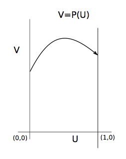
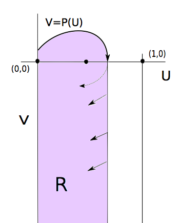
Fig. 1: (left) A “simple solution” (right) Region R

If there exists a point $\xi^{-}\in(0,r)$ with $V(\xi^{-})\leq 0$, then let $\xi_{0}$ be the first point such that $V(\xi)>0$ for $0\leq\xi<\xi_{0}$ and $V(\xi_{0})=0$. By definition $\xi_{0}<r$ and $V^{\prime}(\xi_{0})\leq 0$. Again we cannot have $V^{\prime}(\xi_{0})=0$ since if this is the case, then $V^{\prime}(\xi_{0})=-cV(\xi_{0})-f(U(\xi_{0}))=-f(U(\xi_{0}))=0$ and this implies that $(U(\xi_{0}),V(\xi_{0}))$ is an equilibrium point of (50) which is not the case. Therefore $V^{\prime}(\xi_{0})<0$ (hence $f(U(\xi_{0}))>0$) and in particular for $\xi>\xi_{0}$ but $\xi$ near $\xi_{0}$ we have $U(\xi)<U(\xi_{0})$ and $V(\xi)<0$. Moreover, for $0\leq\xi\leq\xi_{0}$ we have $0\leq U(\xi)\leq U(\xi_{0})<1$ (if $U(\xi_{0})=1$, since $V(\xi_{0})=0$ we will have again another equilibrium point of (50)). Hence, the curve $(U(\xi),V(\xi))$ for $0\leq\xi\leq\xi_{0}$ joins the point $(0,\theta)$ with $(U(\xi_{0}),0)$ with $U(\xi)$ increasing and $V(\xi)>0$, that is this curve can be expressed as $V=P(U)$ for $0\leq U\leq U(\xi_{0})$ for some function $P$.

Consider now the region $R=\{(U,V):0\leq U\leq U(\xi_{0}),\quad-\infty<V<P(U)\}$. Using the direction field of (50), we have that any initial condition starting in the set $R$ either remains for all times in $R$ or it leaves the region $R$ through the boundary $\{(0,V):-\infty<V<0\}$. Since our solution satisfies $U(b)=1$, necessarily has to leave the region $R$ but then there will exist a point $\xi_{1}\in(\xi_{0},b)$ with $U(\xi_{1})=0$ and $V(\xi_{1})<0$, which implies that $U(\xi_{1}+\epsilon)<0$, for $\epsilon>0$ small enough. This is a contradiction with the fact that $0\leq U(\xi)\leq 1$. Hence $V(\xi)>0$ for all $\xi\in[0,r]$. The existence of the function $P$ follows easily now from the fact that $U^{\prime}(\xi)=V(\xi)>0$ for all $\xi\in[0,r]$. ∎

Lemma 11.

The following properties hold:

(i) If $V=P(U)$ is a simple solution then the time it takes to go from the point $(U(\xi_{0}),V(\xi_{0}))$ to $(U(\xi_{1}),V(\xi_{1}))$, that is $\xi_{1}-\xi_{0}$, is given by

$$\xi_{1}-\xi_{0}=\int_{U(\xi_{0})}^{U(\xi_{1})}\frac{dU}{P(U)}.$$

In particular the time it takes to go from $(0,\theta)$ to $(1,\Upsilon)$ is given by

$$r=\int_{0}^{1}\frac{dU}{P(U)}.$$

(ii) If we have two “simple solutions” $V=P_{0}(U)$ and $V=P_{1}(U)$ satisfying $P_{0}(U^{*})<P_{1}(U^{*})$ for some $U^{*}\in[0,1]$, then $P_{0}(U)<P_{1}(U)$ for all $0\leq U\leq 1$.

(iii) If we consider (50) for two constants $c_{0}<c_{1}$ and simple solutions $V=P_{i}(U)$ for the system with $c_{i}$, $i=0,1$, respectively, then if $P_{0}(U^{*})=P_{1}(U^{*})$ for some $0<U^{*}<1$, it is $P^{\prime}_{0}(U^{*})>P^{\prime}_{1}(U^{*})$. In particular the orbits can only cross once (see Figure 2).

(iv) If $\theta>|c|+|f|_{\infty}+1$ where $|f|_{\infty}=\max\{|f(s)|,0\leq s\leq 1\}$ then the solution starting at $(0,\theta)$ is a simple solution joining $(0,\theta)$ with $(1,\Upsilon)$ for some $\Upsilon\geq\theta-|c|-|f|_{\infty}$. Moreover this simple solution $V=P(U)$ satisfies $P(U)\geq\theta-(|c|+|f|_{\infty})U$ for $0\leq U\leq 1$. In particular

$$\int_{0}^{1}\frac{dU}{P(U)}\to 0,\quad\hbox{ as }\theta\to+\infty.$$

(v) There exists $\theta_{0}\geq 0$ such that the solution starting at $(0,\theta)$ for each $\theta>\theta_{0}$ is a simple solution $V=P_{\theta}(U)$ with

$$\int_{0}^{1}\frac{du}{P_{\theta}(U)}\to+\infty,\quad\hbox{ as }\theta\to\theta_{0}^{+}.$$

(vi) For any $\theta_{0}>0$ there exists a $c_{0}=c_{0}(\theta_{0})>0$ such that for all $c>c_{0}$ any “simple solution” starting at $(0,\theta)$ with $\theta>\theta_{0}$ ends at $(1,\Upsilon)$ with $\Upsilon<\theta$. Similarly, there exists a $c_{1}=c_{1}(\theta_{0})<0$ such that for all $c<c_{1}$ any “simple solution” starting at $(0,\theta)$ with $\theta>\theta_{0}$ ends at $(1,\Upsilon)$ with $\Upsilon>\theta$

Proof.

$(i)$ It follows from standard results. Notice that the first equation of (50) reads $\frac{dU}{d\xi}=V=P(U)$ which implies $d\xi=\frac{dU}{P(U)}$ from where we obtain the result via integration.

$(ii)$ This follows from the uniqueness of solutions of the ODE (50).

$(iii)$ Note that $\frac{dP(U)}{dU}=-c+f(U)/P(U)$. Hence, if $P_{0}(U^{*})=P_{1}(U^{*})$, then $P^{\prime}_{0}(U^{*})=-c_{0}+f(U^{*})/P(U^{*})>-c_{1}+f(U^{*})/P(U^{*})=P^{\prime}_{1}(U^{*})$

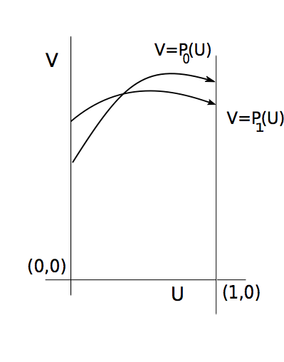
Fig. 2: Two simple solutions $V=P_{0}(U)$, $V=P_{1}(U)$ for $c_{0}<c_{1}$ which crossing.

$(iv)$ In the $(U,V)$ plane, the segment joining $(0,\theta)$ with $(1,\Upsilon^{*})$ is given by $V=(\Upsilon^{*}-\theta)U+\theta$, for $0\leq U\leq 1$. Hence, if $\theta>|c|+|f|_{\infty}+1$ and $\Upsilon^{*}=\theta-|c|-|f|_{\infty}$, the straight line is $V=-(|c|+|f|_{\infty})U+\theta$ and notice that we have $V>1$ for all $(U,V)$ in the segment. But, in this segment, the direction field of the ODE (50) points “toward the right” of the straight line, since the scalar product of its normal vector, $(|c|+|f|_{\infty},1)$, with the direction field $(V,-cV+f(U))$ is

$$(|c|+|f|_{\infty})V-cV+f(U)=V(|c|-c)+|f|_{\infty}V+f(U)>0$$

since if $(U,V)$ lies in the straightline then $V>1$, see Figure 3.

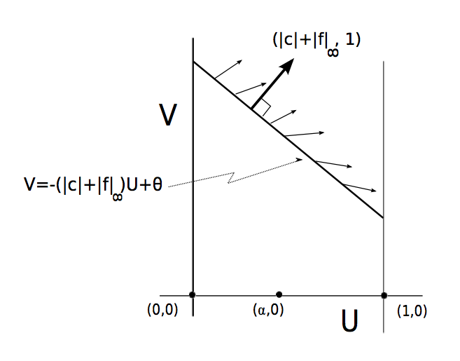
Fig. 3: The segment and the direction field.

This implies that if we start at $(0,\theta)$ then the orbit of the ODE cannot cross this line segment and therefore we will have $P(U)>\theta-(|c|+|f|_{\infty})U$ for all $0\leq U\leq 1$ and in particular it will arrive at a point $(1,\Upsilon)$ with $\Upsilon>\Upsilon^{*}$. The last statement of this item is obvious from the bounds of $P(U)$ and taking $\theta\to+\infty$.

$(v)$ It is clear from $(iv)$ that there exists $\theta_{1}>0$ such that the orbit starting at $(0,\theta)$ for $\theta\geq\theta_{1}$ are all simple solutions. Moreover, from Lemma 10 and the continuous dependence of the solutions of the ODE with respect to the initial conditions, we have that if the solution starting at a point $(0,\theta^{*})$ is a simple solution, then there exists a small $\epsilon>0$ such that for each $\theta\in(\theta^{*}-\epsilon,\theta^{*}+\epsilon)$ the solution is also a simple solution. Let us define

$$\theta_{0}=\inf\{\theta:\hbox{ the orbit starting at }(0,\theta^{+})\forall\theta^{+}>\theta\hbox{ is a simple solution }\}$$

Then, by definition the orbit starting at $(0,\theta_{0})$ is not a simple solution. But, necessarily this orbit satisfies $0\leq U\leq 1$ and, if it reaches a point of the form $(1,\Upsilon)$ in finite time, by Lemma 10 it will also be a simple solution. Therefore by the continuity of the flow, we necessarily have either $\theta_{0}=0$ or $\Upsilon=0$, which leads to

$$\int_{0}^{1}\frac{du}{P_{\theta}(U)}\to+\infty,\quad\hbox{ as }\theta\to\theta_{0}^{+}.$$

$(vi)$ Observe that if $\theta_{0}>0$ and $\theta\geq\theta_{0}$ then, on the horizontal line $V=\theta$, the vector field of the ODE is $(\theta,-c\theta+f(U))$. Therefore, if we choose $c_{0}=|f|_{\infty}/\theta_{0}>0$, then for any $c>c_{0}$ the vector field “points downwards” in this line. This implies that if we start with a solution at $(0,\theta)$ and the solution travels to a point $(1,\Upsilon)$ then the whole orbit lies below the straight line $V=\theta$. Hence, $\Upsilon<\theta$. Similarly for the other case. ∎

We also have another two distinguised solutions with $0\leq U\leq 1$ and $V\geq 0$, which are usually denoted as the “unstable orbit” from the equilibrium $(0,0)$ and the “stable orbit” to the equilibrium $(1,0)$. These are special solutions since they are defined either in an interval of the form $\xi\in(-\infty,r_{0})$ or $\xi\in(r_{1},+\infty)$.

Lemma 12.

There exists a unique value $c^{*}\in\mathbb{R}$ such that the following holds

(i) If $c<c^{*}$ the unique “unstable orbit” emanating from $(0,0)$ with $0\leq U\leq 1$ ends at a point $(U_{0},0)$ for some value $0<U_{0}<1$ and the unique “stable orbit” converging to $(1,0)$ with $0\leq U\leq 1$ starts at a point of the form $(0,\theta_{0})$, with $\theta_{0}>0$.

(ii) If $c>c^{*}$ the unique “unstable orbit” emanating from $(0,0)$ with $0\leq U\leq 1$ ends at a point $(1,\Upsilon_{1})$ for some value $\Upsilon_{1}>0$ and the unique “stable orbit” converging to $(1,0)$ with $0\leq U\leq 1$ starts at a point of the form $(U_{0},0)$.

(iii) If $c=c^{*}$, both orbits coincide and we have a unique orbit with $0\leq U\leq 1$ and $V\geq 0$ which comes out from $(0,0)$ (as $\xi\to-\infty$) and comes in to $(1,0)$ (as $\xi\to+\infty$).

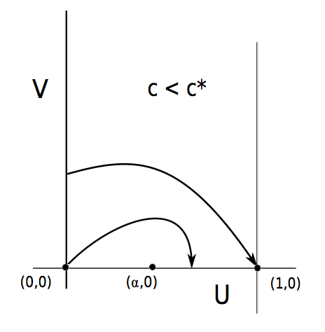
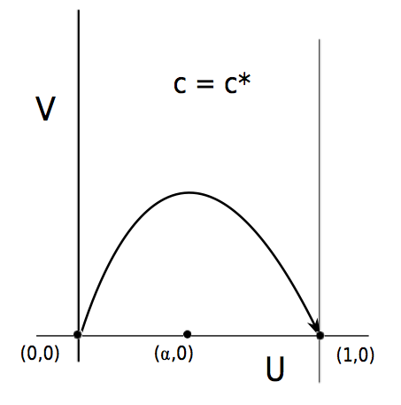
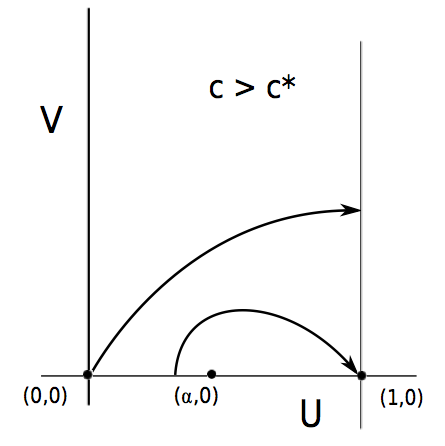
Fig. 4: Phase planes for Lemma 12.

Proof.

The proof is a simple exercise of phase plane techniques and we leave if for the reader. See Figure 4 and the book [19] for details. ∎

Remark 4.

Observe that the value $c^{*}$ from the previous Lemma is the speed of propragation of the travelling wave of problem (1).

With the results above we can prove the first result on existence of solution of (49) with $c$ fixed.

Proposition 13.

For every $c\in\mathbb{R}$, there exists a unique solution $\Phi_{c}$ of (49). Furthermore, $\Phi_{c}$ is strictly monotone, that is, $\Phi^{\prime}(x)>0$ for all $x\in[a,b]$.

Proof.

Observe that $\Phi_{c}$ is a solution of (49) if and only if $(U,V)=(\Phi_{c},\Phi_{c}^{\prime})$ is a simple solution as defined above. But if we consider the value $\theta_{0}$ from Lemma 11 $(v)$ and the simple solution $V=P_{\theta}(U)$ which starts at $(0,\theta)$ then the time it takes to go from $(0,P(0))$ to $(1,P(1))$ is given by

$$r(\theta)=\int_{0}^{1}\frac{dU}{P_{\theta}(U)},$$

which by Lemma 11 $(iv)$ and $(v)$ satisfy that there exists at least one $\theta$ for which $r(\theta)=b-a$. From Lemma 11 $(ii)$ we have the uniqueness. ∎

As we show below, the monotonicity of the equilibrium, yields its asymptotic stability.

Proposition 14.

Let $c\in\mathbb{R}$ and the equilibrium solution $\Phi_{c}$ of (48). Then, there exists $K,a>0$ such that for $\|u_{0}-\Phi_{c}\|_{\infty}$ small enough it holds

$$\|u(\cdot,t)-\Phi_{c}\|_{\infty}\leq Ke^{-at},$$ (51)

for $u$ the solution of (48).

Proof.

We consider the linearization about $\Phi_{c}$ of (57)

$$\left\{\begin{array}[]{l}u_{t}=u_{xx}+cu_{x}+f^{\prime}(\Phi_{c})u,\\ u(a,t)=u(b,t)=0.\end{array}\right.$$ (52)

We need information about the spectrum of the operator

$$L_{0}q:=q^{\prime\prime}+cq^{\prime}+f^{\prime}(\Phi_{c})q,$$ (53)

in $D(L_{0})=\{q\in\,{\mathcal{C}}\,^{2}[a,b]:q(a)=q(b)=0\}$. Deriving the equation in (49) we obtain that $\phi=\Phi^{\prime}_{c}>0$ satisfies the boundary value problem

$$\left\{\begin{array}[]{l}\phi^{\prime\prime}+c\phi^{\prime}_{c}+f^{\prime}(\Phi_{c})\phi=0,\\ \phi^{\prime}(a)+c\phi(a)=0,\qquad\phi^{\prime}(b)+c\phi(b)=0,\end{array}\right.$$ (54)

where the boundary conditions are obtained by evaluating (49) at $\xi=a$ and $\xi=b$ and using that $f(0)=f(1)=0$. The change of variables $z(\xi)=e^{\frac{c}{2}\xi}q(\xi)$ in (54) leads to the self-adjoint problem in $L^{2}(a,b)$

$$\left\{\begin{array}[]{l}\displaystyle-z^{\prime\prime}+\left(\frac{c^{2}}{4}-f^{\prime}(\Phi_{c})\right)z=0,\\[10.00002pt] \displaystyle z^{\prime}(a)+\frac{c}{2}z(a)=0,\qquad z^{\prime}(b)+\frac{c}{2}z(b)=0,\end{array}\right.$$ (55)

For (55), the positive mapping $\xi\to e^{\frac{c}{2}\xi}\phi(\xi)>0$ is an eigenfunction associated to the eigenvalue 0. Then, by Krein-Rutman’s Theorem, 0 is the smallest eigenvalue of the operator

$$Bq:=-z^{\prime\prime}+\left(\frac{c^{2}}{4}-f^{\prime}(\Phi_{c})\right)z,$$ (56)

for the boundary conditions in (55). Then,

$$0 = \min_{H^{1}(a,b)}\frac{\int_{a}^{b}\left[(z^{\prime})^{2}+\left(\frac{c^{4}}{4}-f^{\prime}(\Phi_{c})\right)z^{2}\right]\,d\xi+\frac{|c|}{2}\left(z^{2}(a)-z^{2}(b)\right)}{\int_{a}^{b}z^{2}\,d\xi}$$

$$< \min_{H^{1}_{0}(a,b)}\frac{\int_{a}^{b}\left[(z^{\prime})^{2}+\left(\frac{c^{4}}{4}-f^{\prime}(\Phi_{c})\right)z^{2}\right]\,d\xi}{\int_{a}^{b}z^{2}\,d\xi},$$

so that the smallest eigenvalue of $B$ with homogeneous Dirichlet boundary condition is strictly positive. This implies $\sigma(L_{0})\subset\{z\in\mathbb{C}:{\rm Re}\,z<0\}$, yielding the asymptotic stability of $\Phi_{c}$. ∎

Corollary 15.

With the notations above, we have $\sigma(L_{0})\subset\{z\in\mathbb{C}:{\rm Re}\,z<0\}$.

4.2 The nonlocal problem in a bounded interval

In this section we study the existence of equilibria of the non local equations (9) and (15) restricted to a finite interval with nonhomogeneus Dirichlet boundary conditions. It is immediate to see that the resulting Initial and Boundary Value Problems (IBVP) for both equations are the same, namely:

$$\left\{\begin{array}[]{l}\displaystyle u_{t}=u_{xx}+\lambda(u_{x})u_{x}+f(u),\qquad x\in(a,b),\quad t>0,\\[5.0pt] \displaystyle\lambda(z(\cdot))=-\frac{F(1)}{\|z(\cdot)\|_{L^{2}(a,b)}^{2}}\in\mathbb{R},\\[10.00002pt] u(a,t)=0;\ u(b,t)=1,\qquad t>0,\\ u(x,0)=u_{0}(x),\qquad x\in[a,b],\end{array}\right.$$ (57)

We have the following

Proposition 16.

Problem (57) is locally well posed, in the sense that for any initial data $u_{0}\in H^{1}(a,b)$ with $u_{0}(a)=0$, $u_{0}(b)=1$ there exists a $T=T(u_{0})$ and a unique classical solution $u(x,t)$ defined for the time interval $[0,T(u_{0}))$.

Moreover, if $0\leq u_{0}\leq 1$, then the solution $u(x,t)$ is globally defined and it also satisfies $0\leq u(x,t)\leq 1$.

Proof.

Observe that problem (57) can be rewritten as a more standard problem with homogeneous Dirichlet boundary conditions with the change of variables: $u(x)=w(x)+h(x)$, where the function $h(x)=\frac{x-a}{b-a}$. Notice that if $u(a)=0$, $u(b)=1$, then $w(a)=w(b)=0$ and problem (57) takes the form

$$\left\{\begin{array}[]{l}\displaystyle w_{t}=w_{xx}+F(w)\qquad x\in(a,b),\quad t>0,\\ w(a,t)=w(b,t)=0,\qquad t>0,\\ w(x,0)=w_{0}(x)\equiv u_{0}(x)+h(x),\qquad x\in[a,b],\end{array}\right.$$ (58)

where $F:H^{1}_{0}(a,b)\to L^{2}(a,b)$ is the map defined by $F(w)=\lambda(w_{x}+\frac{1}{b-a})(w_{x}+\frac{1}{b-a})+f(w+h(\cdot))$. We can easily see that this map is well defined, since if $w\in H^{1}_{0}(a,b)$ evaluating in the following expression, we have

$$\left\|w_{x}+\frac{1}{b-a}\right\|_{L^{2}(a,b)}^{2}=\|w_{x}\|^{2}_{L^{2}(a,b)}+\frac{1}{b-a}\geq\frac{1}{b-a}$$

and therefore the denominator in the function $\lambda$ is bounded away from 0 and $\lambda(w_{x}+\frac{1}{b-a})$ is well defined. Moreover, following standard arguments, the map $F$ is Lipschitz on bounded sets of $H^{1}_{0}(a,b)$ which from standard techniques, see [19], we obtain that problem (58) is locally well posed in $H^{1}_{0}(a,b)$ and therefore problem (57) is locally well posed for any initial condition $u_{0}\in H^{1}(a,b)$ satisfying $u_{0}(a)=0$, $u_{0}(b)=1$. Standard regularity results applied to (57) (notice that $\lambda$ is independent of $x$) show that the solution is classical for $t>0$

If we consider now that $0\leq u_{0}\leq 1$, then we may argue by comparison with the constants to show that as long as the solution exists, it will also satisfy $0\leq u\leq 1$. Let us argue by contradiction. Assume the solution is negative at some time $T>0$. Then, for $\epsilon>0$ small enough there exists a $0<t_{\epsilon}\leq T$ such that $u(x,t)>-\epsilon$ for all $x\in[a,b]$, $0\leq t<t_{\epsilon}$ and there exists $x_{\epsilon}\in(a,b)$ such that $u(x_{\epsilon},t_{\epsilon})=-\epsilon$. This implies that $u_{t}(x_{\epsilon},t_{\epsilon})\leq 0$, $u_{xx}(x_{\epsilon},t_{\epsilon})\geq 0$, $u_{x}(x_{\epsilon},t_{\epsilon})=0$ and $f(u(x_{\epsilon},t_{\epsilon}))=f(-\epsilon)>0$. Which is a contradiction. In a similar way we may proceed with the upper bound $u\leq 1$. This shows that, as long as the solution exists we have $0\leq u(x,t)\leq 1$. With standard continuity arguments we show that the solution is globally defined and satisfy the bounds. This concludes the proof of the proposition. ∎

Remark 5.

Notice that although we have been able to obtain a comparison result with the constants 0 and 1, we do not have a general comparison argument for equation (57). That is, if the initial conditions are ordered $u_{0}\leq v_{0}$ we cannot conclude that the solutions satisfy the same ordering for positive times. The lack of these comparison arguments for this equation is very much related to the lack of maximum principles for the associated linear non local operators. This lack is a serious drawback, specially when analyzing the stability properties of the equilibrium of this equation, see Remark 6 below.

Fig. 5: The equilibrium in a bounded domain: (Left) In the phase space $(U,V)$; (Right) As a function of $x$.

The following result provides a characterization of the stationary solutions of (57).

Lemma 17.

A function $\Phi(\cdot)\in H^{1}(a,b)$ with $\Phi(a)=0$, $\Phi(b)=1$ and $0\leq\Phi(x)\leq 1$ is an stationary solution of (57) if and only if $\Phi(\cdot)$ is a solution of (49) with $c=\lambda(\Phi^{\prime})$ and satisfies

$$\Phi^{\prime}(a)=\Phi^{\prime}(b).$$ (59)

Proof.

It is clear that any equilibrium solution $\Phi$ of (57) satisfies (49) for $c=\lambda(\Phi_{x})$. Multiplication by $\Phi^{\prime}$ in the ODE in (49) and integration along $(a,b)$ yields

$$\frac{1}{2}[(\Phi^{\prime}(b))^{2}-(\Phi^{\prime}(a))^{2}]+\lambda(\Phi_{x})\|\Phi^{\prime}\|_{2}^{2}+\langle f(\Phi),\Phi^{\prime}\rangle=0.$$

Using that $\langle f(\Phi),\Phi^{\prime}\rangle=F(1)$ and the definition of $\lambda$ in (57) we obtain that $\Phi$ satisfies (59). ∎

We can proceed now to prove an existence and uniqueness result for stationary solutions of (57).

Theorem 18.

There exists one and only one stationary solution $\Phi$ of (57) with $0\leq\Phi(x)\leq 1$. Moreover, this solution is strictly monotone increasing in $x$.

Proof.

From Lemma 17, a stationary solution $\Phi$ of (57) with $0\leq\Phi(x)\leq 1$ is the first coordinate of a “simple solution” of the ODE

$$\left\{\begin{array}[]{l}U^{\prime}=V,\\ V^{\prime}=-cV-f(U)\end{array}\right.$$ (60)

where $c=\lambda(\Phi^{\prime})=-\frac{F(1)}{\|\Phi^{\prime}\|_{L^{2}(a,b)}^{2}}\in\mathbb{R}$. Lemma 10 proves that $\Phi^{\prime}(x)>0$ for all $x\in[a,b]$ and therefore $\Phi$ is strictly monotone increasing.

Uniqueness is obtained as follows. Assume that there exist two solutions $\Phi_{1}$, $\Phi_{2}$ and denote by $c_{1}=\lambda(\Phi_{1}^{\prime})$, $c_{2}=\lambda(\Phi^{\prime}_{2})$. From the uniqueness of solutions given in Proposition 13, we get that $c_{1}\neq c_{2}$. Then, if we denote by $(U_{1},P(U_{1}))$, $(U_{2},P(U_{2}))$ the two simple solutions associated to $\Phi_{1}$ and $\Phi_{2}$ respectively, from Lemma 11 $(iii)$ and from $P_{1}(0)=P_{1}(1)$, $P_{2}(0)=P_{2}(1)$ we must have that either $P_{1}(U)>P_{2}(U)$ or $P_{1}(U)<P_{2}(U)$ for all $0\leq U\leq 1$. In both cases we have

$$b-a=\int_{0}^{1}\frac{dU}{P_{1}(U)}\neq\int_{0}^{1}\frac{dU}{P_{2}(U)}=b-a$$

which is a contradiction. This shows uniqueness.

Existence is shown as follows. We know from Proposition 13 that for every fixed $c_{0}$ and $r=b-a$ there exists a unique solution $\Phi_{c_{0}}$ of (49), which actually is given by $\Phi_{c_{0}}=U_{0}$ where $(U_{0},V_{0})$ is a “simple solution” joining $(0,\theta_{0})$ with $(1,\Upsilon_{0})$ for some $\theta_{0},\Upsilon_{0}>0$. If it happens that $\theta_{0}=\Upsilon_{0}$, that is $\Phi^{\prime}_{c_{0}}(a)=\Phi^{\prime}_{c_{0}}(b)$, then Lemma 17 shows that this function $\Phi_{c_{0}}$ is the stationary solution we are looking for. If $\theta_{0}\neq\Upsilon_{0}$, let us assume that $\theta_{0}<\Upsilon_{0}$ (the other case is treated similarly). For $c>c_{0}$ and the same $r=b-a$, again by Proposition 13 we have the existence of a solution $\Phi_{c}$ which again is given by $\Phi_{c}=U$ where $(U,V)$ is a “simple solution” joining $(0,\theta)$ with $(1,\Upsilon)$. But since $r$ is the same for both solutions and we have $r=\int_{0}^{1}\frac{dU}{P_{0}(U)}=\int_{0}^{1}\frac{dU}{P(U)}$ then necessarily, both solutions must cross at least at some point and by Lemma 11 they can only cross at one point and it must be satisfied $\theta>\theta_{0}$, $\Upsilon<\Upsilon_{0}$. Moreover, from Lemma 11 we can choose $c_{1}>c_{0}$ large enough such that for this value $c_{1}$ the unique simple solution joining a point of the form $(0,\theta_{1})$ with $(1,\Upsilon_{1})$ in a time $r=b-a$ satisfies $\theta_{1}>\Upsilon_{1}$. By the continuous dependence of the solutions $\Phi_{c}$ with respect to the parameter $c$, we will have that there will exist a value $c^{*}\in(c_{0},c_{1})$ such that the unique solution $\Phi_{c^{*}}$ travelling for a time $r=b-a$ joins a point of the form $(0,\theta^{*})$ with $(0,\Upsilon^{*})$ with $\theta^{*}=\Upsilon^{*}>0$, that is $\Phi^{\prime}(a)=\Phi^{\prime}(b)$. This is the desired solution. ∎

4.3 Convergence of the stationary solutions to the travelling wave as the length of the interval goes to $+\infty$

In this section we will pass to the limit as the interval grows to cover the whole line and we analyze how the solution encountered in Theorem 18 behaves as the length of the interval goes to infinity. The first step is to prove the convergence of the wave speed to the one of the travelling wave. More precisely,

Lemma 19.

Let $\lambda_{r}$ be the unique value given by Theorem 18 for which an equilibrium of (57)-(59) exists on the interval $(a,b)$ with $r=b-a$. Then,

$$|\lambda_{r}-\lambda_{\infty}|\to 0,\qquad\mbox{as }\quad r\to+\infty.$$ (61)

where $\lambda_{\infty}=c^{*}$ from Lemma 12, that is, the speed of propagation of the travelling wave of equation (1).

Proof.

Observe first that the value of $\lambda_{r}$ really depends only on $r=b-a$ and not on $a$ or $b$.

Assume that the result is not true. Then, there is a sequence $\{r_{n}\}_{n\in\mathbb{N}}$ with $r_{n}\to\infty$, as $n\to\infty$, and $\varepsilon>0$ so that if we denote by $\lambda_{n}:=\lambda_{r_{n}}$, then either $\lambda_{n}>\lambda_{\infty}+\epsilon$ or $\lambda_{n}<\lambda_{\infty}-\epsilon$. So let us assume that $\lambda_{n}>\lambda_{\infty}+\varepsilon$, for all $n$, the other case is treated similarly.

Observe that from Lemma 12, in the phase plane associated to the equation (57) for $c=\lambda_{\infty}+\varepsilon$ there is an orbit $(\Phi_{*},\Phi^{\prime}_{*})$ arriving at $(1,0)$ from $(0,\Upsilon^{*})$, for a certain $\Upsilon^{*}>0$. This orbit is also represented as $V=P^{*}(U)$ for $0\leq U\leq 1$. By $(iii)$ of Lemma 11 and (59), none of the orbits $(\Phi_{n},\Phi^{\prime}_{n})$, which are given by $V=P_{n}(U)$, can cross $V=P^{*}(U)$ and it has to be $P_{n}(0)=\Upsilon_{n}>\Upsilon^{*}$, for all $n$. It follows then that $P_{n}(U)>P^{*}(U)$ for all $0\leq U\leq 1$. Furthermore, the graph of the function $V=P_{n}(U)$ is also above the straight line passing through $(1,\Upsilon^{*})$ with slope $(1,-\lambda_{\infty}+\varepsilon)$. This comes from the fact that for $\alpha$ in (3) and $\alpha<u<1$, it is $f(u)>0$ and the field in the phase plane is proportional to $(1,-\lambda-f(u)/v)$ with $-\lambda-f(u)/v<-\lambda$. It follows that the orbit $V=P_{n}(U)$ has to arrive at $(1,\Upsilon_{n})$ from above this line. But then, the time it takes to travel from $(0,\Upsilon_{n})$ to $(1,\Upsilon_{n})$ remains bounded, i.e., by $(i)$ of Lemma 11 it holds

$$r_{n}=b_{n}-a_{n}=\int_{0}^{1}\frac{du}{P_{n}(u)}\leq M(\varepsilon),\qquad\mbox{for all }\quad n\in\mathbb{N}.$$

This is in contradiction with the fact that $r_{n}\to+\infty$. ∎

Lemma 20.

Let $\Phi_{r}$ be the equilibrium obtained in Theorem 18 in the interval $(0,r)$. Then the orbit $(\Phi_{r},\Phi^{\prime}_{r})$ in the phase plane converges to the orbit associated to the travelling wave on the whole line, $(\Phi_{\infty},\Phi^{\prime}_{\infty})$ as $r\to\infty$.

Proof.

Observe that the orbit $(\Phi_{r},\Phi^{\prime}_{r})$ is a simple solution and it is given as $V=P_{r}(U)$, $0\leq U\leq 1$. Moreover, we know that the travelling wave $(\Phi_{\infty},\Phi^{\prime}_{\infty})$ is given as the function $V=P_{\infty}(U)$ for $0\leq U\leq 1$. We will show that $P_{r}\to P_{\infty}$ as $r\to+\infty$.

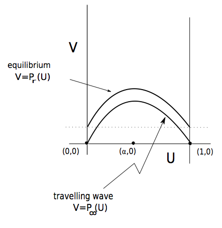
Fig. 6: Convergence of the equilibrium to the travelling wave

Assume the lemma is not true. Then we will have a sequence of $r_{n}\to+\infty$ and a $U_{0}\in[0,1]$ such that $P_{r_{n}}(U_{0})\to V_{0}>P_{\infty}(U_{0})+\delta$ for some $\delta>0$. Notice that we have used the fact that $P_{r}>P_{\infty}$. But we know from Lemma 19 that $\lambda_{r_{n}}\to\lambda_{\infty}$. Hence, by continuous dependence with respect to the initial conditions and with respect to the parameters appearing in the equation, the orbit $(\Phi_{r_{n}},\Phi_{r_{n}}^{\prime})$ converges to the orbit of the ODE with $\lambda=\lambda_{\infty}$ passing by $(U_{0},V_{0})$. Since $V_{0}>P_{\infty}(U_{0})+\delta$ we have that this orbit takes a finite time to go from the line $U=0$ to the line $U=1$. This is a contradiction with the fact that $r_{n}\to+\infty$. ∎

We will normalize the orbit $(\Phi_{r},\Phi_{r}^{\prime})$ so that the time $\xi=0$ will correspond to the unique point for which $\Phi_{r}(0)=1/2$. Hence, we will denote by $a(r)<0<b(r)$ so that $b(r)-a(r)=r$ and $(\Phi_{r}(a(r)),\Phi_{r}^{\prime}(a(r)))=(0,\theta)$ and $(\Phi_{r}(b(r)),\Phi_{r}^{\prime}(b(r)))=(1,\theta)$. In a similar way we may normalize the travelling wave solution so thar $\Phi_{\infty}(0)=1/2$.

We have the following

Proposition 21.

With the notations above, we have both,

$$a(r)\to-\infty,\qquad\hbox{ and }\qquad b(r)\to+\infty.$$

Proof.

Assume one of them is not true. For instance, let us consider that there exists a sequence $r_{n}\to+\infty$ such that $b(r_{n})\to b_{0}<\infty$. This implies that the finite interval $[0,b(r_{n}))$ approaches the finite interval $[0,b_{0})$ and therefore by the continuous dependence of the solutions of the ODE with respect to the parameters and the initial conditions in a finite time interval [18], we will have that $(\Phi_{r_{n}}(b(r_{n})),\Phi_{r_{n}}^{\prime}(b(r_{n})))=(1,\Upsilon_{n})\to(\Phi_{\infty}(b_{0}),\Phi^{\prime}_{\infty}(b_{0}))$ and this implies that $\Phi_{\infty}(b_{0})=1$, which is impossible for any $b_{0}<\infty$, since $\Phi_{\infty}$ is the travelling wave solution.

A similar proof shows that $a(r)\to-\infty$. ∎

We may also prove

Lemma 22.

With the notations above, if we extend the function $\{\Phi_{r}\}$ by 0 to the left of $a(r)$ and by 1 to the right of $b(r)$ (and we still denote this function by $\Phi_{r}$) then

$$\|\Phi_{r}-\Phi_{\infty}\|_{W^{1,\infty}(\mathbb{R})}+\|\Phi_{r}^{\prime}-\Phi_{\infty}^{\prime}\|_{L^{2}(\mathbb{R})}\to 0,\quad\hbox{ as }r\to\infty.$$

Proof.

The convergence in $W^{1,\infty}(\mathbb{R})$ follows directly from Lemma 20. Moreover, notice that since $\lambda_{r}\to\lambda_{\infty}$ and using that $\lambda_{r}=-F(1)/\|\Phi_{r}^{\prime}\|_{L^{2}(\mathbb{R})}^{2}$ and $\lambda_{\infty}=-F(1)/\|\Phi_{\infty}^{\prime}\|_{L^{2}(\mathbb{R})}^{2}$ we have that $\|\Phi_{r}^{\prime}\|_{L^{2}(\mathbb{R})}^{2}\to\|\Phi_{\infty}^{\prime}\|_{L^{2}(\mathbb{R})}^{2}$.

Hence, consider a small enough parameter $\epsilon>0$ and let us fix a large enough interval $[-T,T]$ such that $\|\Phi_{\infty}^{\prime}\|^{2}_{L^{2}(\mathbb{R}\setminus(-T,T))}\leq\epsilon$. Then, from the convergence of the orbits given by Lemma 20, we have that $\lim_{r\to\infty}\|\Phi^{\prime}_{r}-\Phi^{\prime}_{\infty}\|_{L^{2}(-T,T)}^{2}=0$, which implies that $\lim_{r\to\infty}\|\Phi^{\prime}_{r}\|_{L^{2}(-T,T)}^{2}=\|\Phi^{\prime}_{\infty}\|_{L^{2}(-T,T)}^{2}$. Hence,

$$\lim_{r\to\infty}\|\Phi^{\prime}_{r}\|_{L^{2}(\mathbb{R}\setminus(-T,T))}^{2}=\lim_{r\to\infty}\|\Phi^{\prime}_{r}\|_{L^{2}(\mathbb{R})}^{2}-\lim_{r\to\infty}\|\Phi^{\prime}_{r}\|_{L^{2}(-T,T)}^{2}$$

$$\qquad\qquad=\|\Phi^{\prime}_{\infty}\|_{L^{2}(\mathbb{R})}^{2}-\|\Phi^{\prime}_{\infty}\|_{L^{2}(-T,T)}^{2}=\|\Phi^{\prime}_{\infty}\|_{L^{2}(\mathbb{R}\setminus(-T,T))}^{2}\leq\epsilon$$

and therefore,

$$\lim_{r\to\infty}\|\Phi^{\prime}_{r}-\Phi^{\prime}_{\infty}\|_{L^{2}(\mathbb{R})}^{2} \leq \lim_{r\to\infty}\|\Phi^{\prime}_{r}-\Phi^{\prime}_{\infty}\|_{L^{2}(-T,T)}^{2}$$

$$+2\lim_{r\to\infty}\|\Phi^{\prime}_{r}\|_{L^{2}(\mathbb{R}\setminus(-T,T))}^{2}+2\|\Phi^{\prime}_{\infty}\|_{L^{2}(\mathbb{R}\setminus(-T,T))}^{2}\leq 4\epsilon.$$

Since $\epsilon$ is arbitrarily small, we show the Lemma. ∎

5 Asymptotic stability of the stationary solutions of the nonlocal problem

We analyze in this section the stability properties of $\Phi_{r}$, the unique stationary solution of the nonlocal problem (57) in the bounded domain $(a(r),b(r))$. We consider the normalization of this equilibrium explained in the previous subsection, that is $\Phi_{r}(0)=1/2$ and to simplify the notation we will denote the interval by $(a,b)$ instead of $(a(r),b(r))$, unless it is necessary to specify the dependence of the domain in $r$.

The linearization of (57) around $\Phi_{r}$ is given by,

$$\left\{\begin{array}[]{l}w_{t}=w_{xx}+\lambda(\Phi_{r})w_{x}+f^{\prime}(\Phi_{r})w+\pi_{r}(w)\Phi^{\prime}.\qquad x\in(a,b),\ t>0,\\ w(a,t)=w(b,t)=0,\end{array}\right.$$ (62)

with $\pi_{r}$ the linear nonlocal operator

$$\pi_{r}(w)=-2\lambda(\Phi_{r})\frac{\langle w_{x},\Phi^{\prime}_{r}\rangle}{\|\Phi^{\prime}_{r}\|_{2}^{2}}.$$ (63)

The equilibrium $\Phi_{r}$ will be asymptotically stable if the spectrum of the linear operator $L^{r}:D(L^{r})\subset L^{2}(a,b)\to L^{2}(a,b)$ with $D(L^{r})=H^{2}(a,b)\cap H^{1}_{0}(a,b)$, given by

$$L^{r}w:=w_{xx}+\lambda(\Phi_{r})w_{x}+f^{\prime}(\Phi_{r})w+\pi_{r}(w)\Phi^{\prime}_{r}$$ (64)

is contained in the left half of the complex plane. We recall that, by Proposition 14, this is the case for the local operator

$$L_{0}^{r}w:=w_{xx}+\lambda(\Phi_{r})w_{x}+f^{\prime}(\Phi_{r})w,\qquad w\in H^{1}_{0}(a,b).$$ (65)

Observe that $L^{r}w=L_{0}^{r}w+\pi_{r}(w)\Phi^{\prime}_{r}$ and the operator $w\to\pi_{r}(w)\Phi^{\prime}_{r}$ has 1-dimensional rank and can be expressed as

$$w\to\frac{2\lambda(\Phi_{r})}{\|\Phi^{\prime}_{r}\|_{2}^{2}}\Phi^{\prime}_{r}\int w\Phi^{\prime\prime}_{r}$$

This operator is of the form $w\to A\langle w,B\rangle$ with $A(\cdot)=\frac{2\lambda(\Phi_{r})}{\|\Phi^{\prime}_{r}\|_{2}^{2}}\Phi^{\prime}_{r}(\cdot)$ and $B(\cdot)=\Phi^{\prime\prime}_{r}(\cdot)=-\lambda(\Phi_{r})\Phi^{\prime}_{r}(\cdot)-f(\Phi_{r}(\cdot))$ and it is a bounded operator from $L^{2}$ to $L^{2}$ with finite rank. Several properties of the operator $L^{r}$ are inherited from the operator $L_{0}^{r}$: both operators have the same domain, both operators have compact resolvent and therefore the spectrum is only discrete, formed by eigenvalues with finite multiplicity. Nevertheless, all the eigenvalues of operator $L_{0}^{r}$ are real (there is a standard change of variables transforming $L_{0}^{r}$ to a selfadjoint operator) but the operator $L^{r}$ may not have this property. Actually, unless $A\equiv B$ operator $L^{r}$ is not selfadjoint. There are several studies of the spectrum of operators of the form $w\to L_{0}^{r}(w)+A\langle w,B\rangle$ but none of them guarantee us that for our particular case, the spectrum lies in the half complex plane with negative real part. Actually, with the known results in the literature we are not even able to show that the spectrum of $L$ is real. See [9, 10, 11, 14, 15] for results in this direction. One important observation is that in the case that the interval is the complete real line, that is $r=\infty$, then $\Phi^{\prime}_{\infty}$ is the eigenfunction associated to the eigenvalue $0$ for the operator $L_{0}^{\infty}$ and therefore the operator $L^{\infty}=L_{0}^{\infty}+\pi_{\infty}(w)\Phi^{\prime}_{\infty}$ has an special structure that will allow us to show that $\sigma(L^{\infty})=\sigma(L_{0}^{\infty})$ and that $0\in\sigma(L^{\infty})$ with multiplicity 1. As a matter of fact this will give us an alternative proof of the asymptotic stability (with asymptotic phase) of the travelling wave solution of the nonlocal equation in the whole real line (see Theorem 7). The fact that $\Phi^{\prime}_{r}$ is not an eigenfunction of $L_{0}^{r}$, for finite $r$ (as a matter of fact $\Phi^{\prime}_{r}$ does not even satisfy homogeneous Dirichlet boundary conditions) will not permit us to perform a similar argument in a bounded interval. Paradoxically, the analysis in the whole real line is “simpler” than the analysis in a bounded interval.

Nevertheless we will be able to prove the asymptotic stability of the stationary solution of the non local problem (57) for large enough intervals using a perturbative method. The proof is divided into three parts. In the first one we prove some properties of the spectrum of the non local operator (64) on the finite interval $(a,b)$. We next fully analyze the spectrum of the limit operator on the whole line $\mathbb{R}$. Finally, we prove the convergence of the spectrum of $L^{r}$ to the spectrum of $L^{\infty}$ as $r\to+\infty$.

5.1 Spectral properties for any finite interval

The results in this section apply to the stationary solution $\Phi_{r}$ obtained in Theorem 18 in the finite interval $(a,b)$.

Let us start with a general and rough estimate of the spectrum of $L^{r}$ but which is uniform for all $r\geq 1$.

Proposition 23.

There exist $\rho_{0}\in\mathbb{R}^{+}$ and $\phi\in(\pi,2\pi)$ such that if we define the sector $\Sigma_{\rho_{0},\phi}=\{z\in\mathbb{C},|Arg(z-\rho_{0})|>\phi\}$, then $\sigma(L^{r})\subset\Sigma_{\rho_{0},\phi}$ for all $r\geq 1$.

Proof.

Note that $\mu\in\sigma(L^{r})$ if and only if there exists $u\in H^{2}(a,b)\cap H^{1}_{0}(a,b)$ such that $L^{r}u=\mu u$. But the operator $L^{r}$ can be written as $L^{r}u=\Delta u+N(u)$ where $N:H^{1}_{0}(a,b)\to L^{2}(a,b)$ is defined as $N_{r}(u)=\lambda(\Phi_{r})u_{x}+f^{\prime}(\Phi_{r})u+\pi_{r}(u)\Phi^{\prime}_{r}$ and as usual $\Delta u=u_{xx}$. Observe that from Lemmas 19 and 22 we have that the operator $N_{r}$ is bounded uniformly in $r$ for $r\geq 1$, that is, there exists a constant $C_{0}$ independent of $r=b-a$ such that $\|N_{r}u\|_{L^{2}(a,b)}\leq C_{0}\|u\|_{H^{1}_{0}(a,b)}$, for all $r\geq 1$.

On the other hand, standard estimates using the spectral decomposition of $-\Delta$ with Dirichlet boundary conditions in $(a,b)$ show that for $\mu\not\in\mathbb{R}^{-}$

$$\|(-\Delta+\mu I)^{-1}\|^{2}_{\mathcal{L}(L^{2}(a,b),H^{1}_{0}(a,b))}\leq\frac{1}{\hbox{dist}(\mu,\mathbb{R}^{-})}+\frac{|\mu|}{(\mu+|\mu|)^{2}}.$$

Hence, fixing $\phi\in(\pi,2\pi)$ we can choose $\rho_{0}>0$ large enough so that we have

$$\|(-\Delta+\mu I)^{-1}\|^{2}_{\mathcal{L}(L^{2}(a,b),H^{1}_{0}(a,b))}\leq\frac{1}{(2C_{0})^{2}},\quad\forall\mu\in\mathbb{C}\setminus\Sigma_{\rho_{0},\phi}.$$

Therefore, if $\mu\in\mathbb{C}\setminus\Sigma_{\rho_{0},\phi}$ and if there exists $u\in H^{2}(a,b)\cap H^{1}_{0}(a,b)$ such that $L^{r}(u)=\mu u$, then, $u=N\circ(-\Delta+\mu I)^{-1}u$ which implies that $\|u\|_{L^{2}}\leq\|N\|_{\mathcal{L}(H^{1}_{0},L^{2})}\,\|(-\Delta+\mu I)^{-1}\|_{\mathcal{L}(L^{2},H^{1}_{0})}\|u\|_{L^{2}}\leq C_{0}\frac{1}{2C_{0}}\|u\|_{L^{2}}\leq 1/2\|u\|_{L^{2}}$ and therefore $u\equiv 0$, which implies that $\mu\not\in\sigma(L^{r})$. ∎

This rough estimate of the spectrum of $L^{r}$ allows us to prove that if there is an eigenvalue of $L^{r}$ with positive real part, then necessarily we will have that it is uniformly bounded in $r$, that is

Corollary 24.

With the notations of the previous proposition, we have that for any value $\nu>0$, we have

$$\{z\in\sigma(L^{r}),{\rm Re}\,z\geq-\nu\}\subset\{z\in\mathbb{C},-\nu\leq{\rm Re}\,z\leq\rho_{0},|Im(z)|\leq(\rho_{0}+\nu)\sin(\phi)\}.$$

Lemma 25.

Let $\mu\in\sigma(L^{r})\bigcap\rho(L_{0}^{r})$. Then, $\mu$ is at most a geometrically simple eigenvalue of $L^{r}$, that is, $Ker(L^{r}-\mu I)$ is one dimensional. Moreover, the associated eigenspace is generated by $y$, the unique solution of

$$(L_{0}^{r}-\mu I)y=\Phi^{\prime}_{r},$$ (66)

and

$$\pi_{r}(y)=-2\lambda\frac{\langle y^{\prime},\Phi^{\prime}_{r}\rangle}{\|\Phi^{\prime}_{r}\|_{2}^{2}}=-1.$$ (67)

Proof.

Let $w\neq 0$ be such that $L^{r}w=\mu w$. Then,

$$0=(L^{r}-\mu I)w=(L_{0}^{r}-\mu I)w+\pi_{r}(w)\Phi^{\prime}_{r}=(L_{0}^{r}-\mu I)(w+\pi_{r}(w)y),$$

so that

$$w=-\pi_{r}(w)y.$$ (68)

The above implies that $\mu$ is at most a simple eigenvalue of $L^{r}$ with eigenspace generated by $y$. Identity (67) follows after applying the linear operator $\pi_{r}$ in (68). ∎

However, it will be still useful for the last part of our argument.

Proposition 26.

There is no real eigenvalue $\mu\geq 0$ in $\sigma(L^{r})$.

Proof.

Let us assume that there exists an eigenvalue $\mu\geq 0$ of $L^{r}$. Since $\sigma(L_{0}^{r})\subset\{z\in\mathbb{C}:{\rm Re}\,z<0\}$ (see Proposition 14 and Corollary 15) then $\mu\in\rho(L_{0}^{r})$. Let $y$ be as in (66) for this value of $\mu$. Then, by definition, $y$ satisfies

$$y^{\prime\prime}+\lambda y^{\prime}+(f^{\prime}(\Phi_{r})-\mu)y=\Phi^{\prime}_{r}.$$ (69)

Multiplying in (69) by $\Phi^{\prime}_{r}$ and integrating in $(a,b)$ we have

$$\langle y^{\prime\prime},\Phi^{\prime}\rangle+\lambda\langle y^{\prime},\Phi^{\prime}_{r}\rangle+\langle f^{\prime}(\Phi_{r})y,\Phi^{\prime}_{r}\rangle-\mu\langle y,\Phi^{\prime}_{r}\rangle=\|\Phi^{\prime}_{r}\|^{2}.$$

But

$$\langle f^{\prime}(\Phi_{r})y,\Phi^{\prime}_{r}\rangle=-\langle y^{\prime},f(\Phi_{r})\rangle=\langle y^{\prime},\Phi^{\prime\prime}_{r}+\lambda\Phi^{\prime}_{r}\rangle,$$

so that

$$\langle y^{\prime\prime},\Phi_{r}^{\prime}\rangle+\langle y^{\prime},\Phi_{r}^{\prime\prime}\rangle+2\lambda\langle y^{\prime},\Phi_{r}^{\prime}\rangle-\mu\langle y,\Phi_{r}^{\prime}\rangle=\|\Phi_{r}^{\prime}\|^{2}.$$

Then, by (67), it holds

$$\langle y^{\prime\prime},\Phi_{r}^{\prime}\rangle+\langle y^{\prime},\Phi_{r}^{\prime\prime}\rangle=\mu\langle y,\Phi_{r}^{\prime}\rangle\leq 0,$$ (70)

where the inequality follows from the maximum principle applied to $-L^{r}_{0}y+\mu y=-\Phi^{\prime}_{r}$ and taking into account that $\Phi^{\prime}_{r}>0$, so that $y<0$ in $(a,b)$. But, from Lemma 17, we know that $\theta:=\Phi^{\prime}_{r}(a)=\Phi^{\prime}_{r}(b)>0$, which implies, together with (70), that

$$\langle y^{\prime\prime},\Phi^{\prime}_{r}\rangle+\langle y^{\prime},\Phi^{\prime\prime}_{r}\rangle=y^{\prime}\Phi^{\prime}_{r}|_{a}^{b}=\theta(y^{\prime}(b)-y^{\prime}(a))\leq 0,$$

and therefore $y^{\prime}(b)\leq y^{\prime}(a)$. But, on the other hand, the fact that $y<0$ in $(a,b)$ together with $y=0$ in $x=a,b$, imply that $y^{\prime}(a)\leq 0\leq y^{\prime}(b)$. Therefore $y^{\prime}(a)=y^{\prime}(b)=0$. But this is impossible, since if, for instance, $y^{\prime}(a)=0$, then $y$ is a solution of the initial value problem $L^{r}_{0}y=\Phi^{\prime}_{r}$ in $(a,b)$ with $y(a)=y^{\prime}(a)=0$ and this implies that $y^{\prime\prime}(a)=\Phi^{\prime}_{r}(a)>0$, so that with $x$ near $a$ we have $y>0$ which is not true. ∎

Remark 6.

i) This proposition would be enough to finish the proof of the asymptotic stability if the non local operator $L^{r}$ had the property that the eigenvalue with the largest real part were real. For instance, this could be obtained if $L^{r}$ satisfies the hypothesis for a Krein-Rutmann type of theorem. But for this theorem we need to have maximum principles and are unable to prove this principles for this nonlocal operator.

ii) Observe that this proposition does not exclude the possibility of having complex eigenvalues with positive real part. Actually, we will be able to exclude this possibility only for large enough intervals by using a peturbative argument. The fact that this operator may present complex eigenvalues with positive real parts for some intervals $(a,b)$ is an open interesting question.

5.2 Spectrum of the nonlocal problem in the whole line

In this section we analyze in detail the spectrum of the corresponding nonlocal operator in the entire real line. This operator is the one associated to the linearization around the asymptotic equilibrium $\Phi_{\infty}$, that is,

$$L^{\infty}(w)=w_{xx}+\lambda(\Phi_{\infty})w_{x}+f^{\prime}(\Phi_{\infty})w+\pi_{\infty}(w)\Phi_{\infty}^{\prime},$$ (71)

where now $\pi_{\infty}$ stands for the linear operator

$$\pi_{\infty}(w)=\frac{-2\lambda(\Phi_{\infty})}{\|U^{\prime}\|_{2}^{2}}\langle U^{\prime},w_{x}\rangle.$$ (72)

We will use several important properties of the spectrum of the local operator

$$L_{0}^{\infty}w:=w^{\prime\prime}+\lambda(\Phi_{\infty})w^{\prime}+f^{\prime}(\Phi_{\infty})w,$$ (73)

We have the following,

Lemma 27.

With respect to the spectrum of $L_{0}^{\infty}$, defined by (73), we have

(i) The essential spectrum $\sigma_{ess}(L_{0}^{\infty})\subset\{z\in\mathbb{C}:{\rm Re}\,z\leq\max\{f^{\prime}(0),f^{\prime}(1)\}\}$.

(ii) There exists $0<\nu<-\max\{f^{\prime}(0),f^{\prime}(1)\}\}$ such that $\sigma(L_{0}^{\infty})\cap\{z\in\mathbb{C}:{\rm Re}\,z\geq-\nu\}=\{0\}$ and the eigenfunction associated to $\mu=0$ is $\Phi^{\prime}_{\infty}$.

(iii) There is no solution $w\in H^{2}(\mathbb{R})$ of $L_{0}^{\infty}w=\Phi^{\prime}_{\infty}$. Therefore, $0$ is an algebraically simple eigenvalue of $L_{0}^{\infty}$, that is, $Ker((L_{0}^{\infty})^{2})=Ker(L_{0}^{\infty})=$span$\{\Phi^{\prime}_{\infty}\}$

We refer to Appendix B for a proof of this result.

Both $L_{0}^{\infty}$ and $L^{\infty}$ are sectorial operators and are related by

$$L^{\infty}(u)=L_{0}^{\infty}(u)+\pi_{\infty}(u)\cdot\Phi_{\infty}^{\prime}$$ (74)

In the following Proposition we show that $L^{\infty}$ enjoys the same spectral properties as $L_{0}^{\infty}$.

Proposition 28.

Let $L^{\infty}$ be the linear operator defined above in (74). Then $\sigma(L^{\infty})=\sigma(L_{0}^{\infty})$ and $0\in\sigma(L^{\infty})$ is an algebraically simple eigenvalue of $L^{\infty}$. In particular the three items $(i)$, $(ii)$ and $(iii)$ from Lemma 27 also hold for $L^{\infty}$.

Proof.

By applying integration by parts it is easy to see that $\pi_{\infty}(\Phi^{\prime}_{\infty})=0$. Then, since $L_{0}^{\infty}\Phi^{\prime}_{\infty}=0$, we also have that $L^{\infty}\Phi^{\prime}_{\infty}=0$, so that $0\in\sigma(L^{\infty})$ with associated eigenfunction $\Phi^{\prime}_{\infty}$. In order to see that 0 is a simple eigenvalue of $L^{\infty}$, let us consider first $\phi\in D(L^{\infty})$ with $L^{\infty}\phi=0$. In case $\pi_{\infty}(\phi)=0$, then it is $L_{0}^{\infty}\phi=0$ and, since 0 is a simple eigenvalue for $L_{0}^{\infty}$, it must be $\phi\sim\phi^{\prime}_{\infty}$. Let us assume now that $\pi_{\infty}(\phi)\neq 0$. Then, it follows $L_{0}^{\infty}\phi=-\pi_{\infty}(\phi)\Phi^{\prime}_{\infty}$, which is impossible by Lemma 27 $(iii)$. With a very similar argument it is possible to show that there is no $w\in H^{2}$ satisfying $L^{\infty}w=\phi^{\prime}_{\infty}$. Hence, 0 is an algebraically simple eigenvalue of $L^{\infty}$.

We show now that $\rho(L_{0}^{\infty})\subset\rho(L^{\infty})$. So, let $\mu\in\rho(L_{0}^{\infty})$, $f\in X$ and $w_{f}\in D(L_{0}^{\infty})$ be the unique element of $D(L_{0}^{\infty})$ such that

$$L_{0}^{\infty}w_{f}-\mu w_{f}=f.$$ (75)

If $\pi_{\infty}(w_{f})=0$, then $L^{\infty}w_{f}-\mu w_{f}=f$. In case $\pi_{\infty}(w_{f})\neq 0$, we can consider

$$w^{*}=w_{f}+\frac{1}{\mu}\pi_{\infty}(w_{f})\Phi^{\prime}_{\infty},$$ (76)

since we already know that $\mu\neq 0$. Then, using that $L_{0}^{\infty}\Phi^{\prime}_{\infty}=\pi_{\infty}(\Phi^{\prime}_{\infty})=0$ and (74), one gets

$$L^{\infty}w^{*}-\mu w^{*}=f.$$ (77)

This proves that $L^{\infty}-\mu I$ is onto.

Let us assume now that there exist two elements $w_{1}^{*},w_{2}^{*}\in D(L^{\infty})$ with

$$L^{\infty}w_{j}^{*}-\mu w_{j}^{*}=f,\qquad\mbox{ for }\ j=1,2.$$

Then

$$L_{0}^{\infty}w_{j}^{*}-\mu w_{j}^{*}=-\pi_{\infty}(w_{j}^{*})\Phi^{\prime}_{\infty}+f,\qquad\mbox{ for }\ j=1,2.$$

From the above it is clear that $\pi_{\infty}(w_{1}^{*})=\pi_{\infty}(w_{2}^{*})$ implies $w_{1}^{*}=w_{2}^{*}$, since $L_{0}^{\infty}-\mu I$ is one to one. In case $\pi_{\infty}(w_{1}^{*})\neq\pi_{\infty}(w_{2}^{*})$, we consider $\bar{w}=w_{1}^{*}-w_{2}^{*}$ and we get $L_{0}^{\infty}\bar{w}-\mu\bar{w}=-\pi_{\infty}(\bar{w})\Phi^{\prime}_{\infty},$, which implies $\bar{w}=-\pi_{\infty}(\bar{w})(L_{0}^{\infty}-\mu I)^{-1}\Phi^{\prime}_{\infty}.$ But $(L_{0}^{\infty}-\mu I)^{-1}\Phi^{\prime}_{\infty}=-\Phi^{\prime}_{\infty}/\mu$ and therefore $\bar{w}\sim\Phi^{\prime}_{\infty}$ and $\pi_{\infty}(\bar{w})=0$, which is a contradiction.

The fact that $(L^{\infty}-\mu I)^{-1}$ is bounded is clear from the expression

$$(L^{\infty}-\mu I)^{-1}f=(L_{0}^{\infty}-\mu I)^{-1}f+\frac{1}{\mu}\pi_{\infty}(w_{f})\Phi^{\prime}_{\infty}.$$

which is obtained from (76)-(77). This shows that $\rho(L_{0}^{\infty})\subset\rho(L^{\infty})$.

The proof of the other inclusion $\rho(L^{\infty})\subset\rho(L_{0}^{\infty})$ is completely symmetrical to this one, once we know that $0$ is also a simple eigenvalue of $L^{\infty}$. We just need to express $L_{0}^{\infty}=L-\pi_{\infty}\Phi^{\prime}_{\infty}$ and remake the proof we have just shown. ∎

Remark 7.

(i) In particular, we have that the spectrum of $L^{\infty}$ apart from $0$ is located in the left half plane, i.e., there exists $\nu>0$, such that

$$\sup\{{\rm Re}\,\mu:\mu\in\sigma(L^{\infty}),\ \mu\neq 0\}=-\nu,\quad\mbox{ for some }\ \nu>0.$$ (78)

(ii) Observe also that since the operator $u\to\pi_{\infty}(u)\Phi^{\prime}_{\infty}$ is a compact operator then $\sigma_{ess}(L_{\infty})=\sigma_{ess}(L_{\infty}^{0})\subset\{z\in\mathbb{C}:{\rm Re}\,z\leq\max\{f^{\prime}(0),f^{\prime}(s)\}\,\}$, see [19].

5.3 Spectral convergence and asymptotic stability of the stationary solution

In this subsection we will end up proving the asymptotic stability of the stationary solution $\Phi_{r}$ of the non local problem. We will obtain this via a convergence of the spectrum of the operator $L^{r}$ to $L^{\infty}$. In order to prove this spectral convergence we will use the theory of regular convergence developed in [29, 30, 31] and the related results in [4]. The necessary definitions are given below.

Let $E$ and $F$ denote separable Banach spaces and let $\{E_{r}\}_{r>0}$ and $\{F_{r}\}_{r>0}$ be families of separable Banach spaces. Let $\{p_{r}\}_{r>0}$, $p_{r}\in\mathcal{L}(E,E_{r})$ and $\{q_{r}\}_{r\in\mathbb{N}}$, $q_{r}\in\mathcal{L}(F,F_{r})$ be linear bounded operators such that

$$\begin{array}[]{l}\lim_{r\to\infty}\|p_{r}e\|_{E_{r}}\to\|e\|_{E},\qquad\mbox{for every }\ e\in E\quad\mbox{and }\\ \lim_{r\to\infty}\|q_{r}f\|_{F_{r}}\to\|f\|_{F},\qquad\mbox{for every }\ f\in F.\end{array}$$ (79)

A family $\{e_{r}\}_{r>0}$, $e_{r}\in E_{r}$, is said to be $\,{\mathcal{P}}\,$-convergent to $e\in E$, written $e_{r}\stackrel{{\scriptstyle\,{\mathcal{P}}\,}}{{\rightarrow}}e$, if

$$\lim_{r\to\infty}\|e_{r}-p_{r}e\|_{E_{r}}=0.$$ (80)

A family $\{e_{r}\}_{r>0}$, $e_{r}\in E_{r}$, is said to be $\,{\mathcal{P}}\,$-compact if every infinite sequence contains a $\,{\mathcal{P}}\,$-convergent subsequence. Analogous definitions apply for $\,{\mathcal{Q}}\,$-convergence and $\,{\mathcal{Q}}\,$-compactness.

A family of bounded linear operators $\{A_{r}\}_{r>0}$, $A_{r}\in\mathcal{L}(E_{r},F_{r})$, is said to be $\,{\mathcal{P}Q}\,$-convergent to $A\in\mathcal{L}(E,F)$, written $A_{r}\stackrel{{\scriptstyle\,{\mathcal{P}Q}\,}}{{\longrightarrow}}A$, as $r\to\infty$, if $e_{r}\stackrel{{\scriptstyle\,{\mathcal{P}}\,}}{{\rightarrow}}e$ implies $A_{r}e_{r}\stackrel{{\scriptstyle\,{\mathcal{Q}}\,}}{{\rightarrow}}Ae$, as $r\to\infty$. The $\,{\mathcal{P}Q}\,$-convergence is said to be regular if for every bounded sequence $\{e_{r}\}_{r>0}$, $e_{r}\in E_{r}$, such that the sequence $\{A_{r}e_{r}\}_{r>0}$ is $\,{\mathcal{Q}}\,$-compact, it turns out that $\{e_{r}\}_{r>0}$ is $\,{\mathcal{P}}\,$-compact.

The relevance of the $\,{\mathcal{P}Q}\,$ regular convergence is that we obtain the following result, which is taken from [29, 30, 31] in a simplified version.

Theorem 29.

Assume we have the family of operators $A(s)=A-sB\in\mathcal{L}(E,F)$ and $A_{r}(s)=A_{r}-sB_{r}\in\mathcal{L}(E_{r},F_{r})$ where the parameter $s\in S$, a bounded subset of the complex plane $\mathbb{C}$, which satisfy the following hypotheses:

(i) $A_{r}(s)$ $\,{\mathcal{P}Q}\,$-converges regularly to $A(s)$ for all $s\in S$.

(ii) For each $s\in S$ the operators $A_{r}(s)$ and $A(s)$ are Fredholm with index 0.

(iii) There exists $s^{\prime}\in S$ such that $Ker(A(s^{\prime}))=\{0\}$.

(iv) There exists a constant $C=C(S)$ such that $\|A_{r}(s)\|_{\mathcal{L}(E_{r},F_{r})}\leq C$ for all $r\geq 0$.

Then, if we denote by $W(s_{0})$ the “root subspace” associated to $A(s_{0})$, that is, the linear space generated by the chain of vectors $\{e_{0},e_{1},\ldots,e_{k},\ldots\}$ defined as,

$$(A-s_{0}B)e_{0}=0,\quad(A-s_{0}B)e_{1}=Be_{0},\ldots\quad(A-s_{0}B)e_{k}=Be_{k-1},\ldots$$

and if we denote by $W_{r}(s_{0},\delta)$ the hull of all “root subspaces” associated to $A_{r}(s)$ for all $|s-s_{0}|\leq\delta$, $s\in S$, then we have that for $\delta>0$ small enough

$$\hbox{dist}_{H}(W_{r}(s_{0},\delta),W(s_{0}))\to 0,\quad\mbox{ as }r\to+\infty,$$

and therefore there exists a $\delta>0$ small such that

$$\hbox{dim}(W_{r}(s_{0},\delta))=dim(W(s_{0})),\quad\mbox{ as }r\to+\infty.$$

Proof.

See the proof in [29, 30, 31]. ∎

Let us write our operators in such a way that we can obtain the regular convergence. Consider the following setting. Let $E=H^{1}(\mathbb{R},\mathbb{C}^{2})$ and $F=L^{2}(\mathbb{R},\mathbb{C}^{2})$, the spaces in the whole real line. Also, $E_{r}=H^{1}(I_{r},\mathbb{C}^{2})$ and $F_{r}=L^{2}(I_{r},\mathbb{C}^{2})\times\mathbb{C}^{2}$, the spaces in the finite interval $I_{r}$ and observe that the space $F_{r}$ has two extra coordinates.

Define the family of linear operators $p_{r}:E\to E_{r}$ and $q_{r}:F\to F_{r}$ as

$$p_{r}\begin{pmatrix}u\\ v\end{pmatrix}=\begin{pmatrix}u_{|I_{r}}\\ v_{|I_{r}}\end{pmatrix}$$

and

$$q_{r}\begin{pmatrix}u\\ v\end{pmatrix}=\begin{pmatrix}u_{|I_{r}}\\ v_{|I_{r}}\\ 0\\ 0\end{pmatrix}.$$

Consider the family of operators $A_{\infty}^{s},A_{0,\infty}^{s},\Pi_{\infty}:E\to F$, defined as,

$$A_{\infty}^{s}\begin{pmatrix}u\\ v\end{pmatrix}=\begin{pmatrix}u_{x}\\ v_{x}\end{pmatrix}+\begin{pmatrix}0&-I\\ f^{\prime}(\Phi_{\infty})-s&\lambda_{\infty}\end{pmatrix}\begin{pmatrix}u\\ v\end{pmatrix}+\begin{pmatrix}0\\ \pi_{\infty}(u)\Phi^{\prime}_{\infty}\end{pmatrix},$$

$$A_{0,\infty}^{s}\begin{pmatrix}u\\ v\end{pmatrix}=\begin{pmatrix}u_{x}\\ v_{x}\end{pmatrix}+\begin{pmatrix}0&-I\\ f^{\prime}(\Phi_{\infty})-s&\lambda_{\infty}\end{pmatrix}\begin{pmatrix}u\\ v\end{pmatrix},$$

and

$$\Pi_{\infty}\begin{pmatrix}u\\ v\end{pmatrix}=\begin{pmatrix}0\\ \pi_{\infty}(u)\Phi^{\prime}_{\infty}\end{pmatrix}$$

and observe that $A_{\infty}^{s}=A_{0,\infty}^{s}+\Pi_{\infty}$. Moreover, the operator $A^{s}_{0,\infty}$ is a local operator. The operator $A_{\infty}^{s}$ can also be decomposed as

$$A_{\infty}^{s}=A_{\infty}^{0}-sB_{\infty},$$ (81)

where

$$B_{\infty}\begin{pmatrix}u\\ v\end{pmatrix}=\begin{pmatrix}0\\ u\end{pmatrix}.$$ (82)

With respect to the operators in a bounded interval, we define, $A^{s}_{r},A^{s}_{0,r},\Pi_{r}:E_{r}\to F_{r}$ as

$$A_{r}^{s}\begin{pmatrix}u\\ v\end{pmatrix}=\begin{pmatrix}u_{x}\\ v_{x}\\ 0\\ 0\end{pmatrix}+\begin{pmatrix}0&-I\\ f^{\prime}(\Phi_{r})-s&\lambda_{r}\\ 0&0\\ 0&0\end{pmatrix}\begin{pmatrix}u\\ v\end{pmatrix}+\begin{pmatrix}0\\ \pi_{r}(u)\Phi^{\prime}_{r}\\ 0\\ 0\end{pmatrix}+\begin{pmatrix}0\\ 0\\ u(a(r))\\ u(b(r))\end{pmatrix},$$

$$A_{0,r}^{s}\begin{pmatrix}u\\ v\end{pmatrix}=\begin{pmatrix}u_{x}\\ v_{x}\\ 0\\ 0\end{pmatrix}+\begin{pmatrix}0&-I\\ f^{\prime}(\Phi_{r})-s&\lambda_{r}\\ 0&0\\ 0&0\end{pmatrix}\begin{pmatrix}u\\ v\end{pmatrix}+\begin{pmatrix}0\\ 0\\ u(a(r))\\ u(b(r))\end{pmatrix}$$

and

$$\Pi_{r}\begin{pmatrix}u\\ v\end{pmatrix}=\begin{pmatrix}0\\ \pi_{r}(u)\Phi^{\prime}_{r}\\ 0\\ 0\end{pmatrix}$$

and observe that in a similar way, we have

$$A_{r}^{s}=A_{r}^{0}-sB_{r},$$ (83)

with

$$B_{r}\begin{pmatrix}u\\ v\end{pmatrix}=\begin{pmatrix}0\\ u\\ 0\\ 0\end{pmatrix}.$$

We have the following,

Proposition 30.

With the notation above, for any $s\in\{{\rm Re}\,s>-\nu\}$, we have

(i) The sequence of operators $A^{s}_{0,r}$ $\,{\mathcal{P}Q}\,$-converges regularly to $A^{s}_{0,\infty}$ as $r\to\infty$.

(ii) The sequence of operators $A^{s}_{r}$ $\,{\mathcal{P}Q}\,$-converges regularly to $A^{s}_{\infty}$ as $r\to\infty$.

(iii) The family of operators $A^{s}_{\infty}$, $A^{s}_{r}$ are Fredholm operators of index 0.

Proof.

$(i)$ Let us define the auxiliary operator $\tilde{A}_{0,r}^{s}:E_{r}\to F_{r}$ which is given by,

$$\tilde{A}_{0,r}^{s}\begin{pmatrix}u\\ v\end{pmatrix}=\begin{pmatrix}u_{x}\\ v_{x}\\ 0\\ 0\end{pmatrix}+\begin{pmatrix}0&-I\\ f^{\prime}(\Phi_{\infty})-s&\lambda_{\infty}\\ 0&0\\ 0&0\end{pmatrix}\begin{pmatrix}u\\ v\end{pmatrix}+\begin{pmatrix}0\\ 0\\ u(a(r))\\ u(b(r))\end{pmatrix}$$

where we consider that $f^{\prime}(\Phi_{\infty})$ is restricted to the interval $I_{r}$. Notice that $A_{0,r}^{s}=\tilde{A}_{0,r}^{s}+B_{r}$ where

$$B_{r}\begin{pmatrix}u\\ v\end{pmatrix}=\begin{pmatrix}0&0\\ -f^{\prime}(\Phi_{\infty})+f^{\prime}(\Phi_{r})&-\lambda_{\infty}+\lambda_{r}\\ 0&0\\ 0&0\end{pmatrix}\begin{pmatrix}u\\ v\end{pmatrix}$$

and observe that $\|B_{r}\|_{\mathcal{L}(E_{r},F_{r})}\to 0$ as $r\to+\infty$, since $\lambda_{r}\to\lambda_{\infty}$ and $\|f^{\prime}(\Phi_{\infty})-f^{\prime}(\Phi_{r})\|_{L^{\infty}}\to 0$, see Lemmas 19 and 22.

But from [4] we know that $\tilde{A}_{0,r}^{s}$ $\,{\mathcal{P}Q}\,$-converges regularly to $A_{0,\infty}^{s}$. This convergence is not trivial at all and it uses deep techniques like exponential dichotomy. Also, it is worthwile to mention that this result is implicit in the work of Beyn and Lorenz [3].

The fact now that $\|B_{r}\|_{\mathcal{L}(E_{r},F_{r})}\to 0$ implies easily the result.

$(ii)$ Once we have obtained the convergence for the “local” operators and recalling that $A_{r}^{s}=A_{0,r}^{s}+\Pi_{r}$, $A_{\infty}^{s}=A_{0,\infty}^{s}+\Pi_{\infty}$ we obtain the $\,{\mathcal{P}Q}\,$ regular convergence from the $\,{\mathcal{P}Q}\,$ regular convergence of $A_{0,r}^{s}$ to $A_{0,\infty}^{s}$, the $\,{\mathcal{P}Q}\,$ convergence of $\Pi_{r}$ to $\Pi_{\infty}$ and the fact that both $\Pi_{r}$ and $\Pi_{\infty}$ are operators with a 1-dimensional rank.

$(iii)$ Let us divide the proof in two parts.

$(iii$-1) $A_{r}^{s}$ is Fredholm with index 0. Operator $A_{r}^{s}$ is defined in the finite interval $I_{r}$ where we have the compact embedding $H^{1}(I_{r},\mathbb{C})\hookrightarrow L^{2}(I_{r},\mathbb{C})$. This implies in particular that the operator

$$\begin{pmatrix}u\\ v\end{pmatrix}\longrightarrow A_{r}^{s}\begin{pmatrix}u\\ v\end{pmatrix}-\begin{pmatrix}u_{x}\\ v_{x}\\ 0\\ 0\end{pmatrix}=\begin{pmatrix}0&-I\\ f^{\prime}(\Phi_{r})-s&\lambda_{r}\\ 0&0\\ 0&0\end{pmatrix}\begin{pmatrix}u\\ v\end{pmatrix}+\begin{pmatrix}0\\ 0\\ u(a(r))\\ u(b(r))\end{pmatrix}$$

is a compact operator from $E_{r}$ to $F_{r}$, since it is a bounded operator from $L^{2}(I_{r},\mathbb{C})\times L^{2}(I_{r},\mathbb{C})$ to $F_{r}$.

Hence, the operator $A^{s}_{r}:E_{r}\to F_{r}$ is a Fredholm operator of index 0 if and only if the bounded operator $D_{r}:E_{r}\to F_{r}$, given by

$$D_{r}\begin{pmatrix}u\\ v\end{pmatrix}=\begin{pmatrix}u_{x}\\ v_{x}\\ 0\\ 0\end{pmatrix}$$

is a Fredholm operator of index 0. But this is very easy to show, since $Ker(D_{r})=\{(u,v)\in E_{r}:u=constant,v=constant\}\equiv\mathbb{C}\times\mathbb{C}$ and therefore dim$(Ker(D_{r}))=2$. Moreover, the rank of $D_{r}$ is $L^{2}(I_{r})\times L^{2}(I_{r})\times\{0\}\times\{0\}\subset F_{r}$ which has codimension 2.

$(iii$-2) $A_{\infty}^{s}$ is Fredholm with index 0. Observe that the operator $A_{\infty}^{s}$ can be decomposed as $A^{s}_{\infty}=F^{s}_{\infty}+K_{\infty}+\Pi_{\infty}$ where $\Pi_{\infty}$ is given as above (and is a compact operator since it has rank=1), and the other two operators are given as

$$K_{\infty}\begin{pmatrix}u\\ v\end{pmatrix}=\begin{pmatrix}0\\ [f^{\prime}(\Phi_{\infty})-V(\cdot)]u\end{pmatrix},$$

and

$$F_{\infty}^{s}\begin{pmatrix}u\\ v\end{pmatrix}=\begin{pmatrix}u_{x}\\ v_{x}\end{pmatrix}+\begin{pmatrix}0&-I\\ V(\cdot)-s&\lambda_{\infty}\end{pmatrix}\begin{pmatrix}u\\ v\end{pmatrix},$$

where the potential $V(x)$ is piecewise constant and it is defined as

$$V(x)=\left\{\begin{array}[]{l}f^{\prime}(0),\quad x\in(-\infty,0],\\ f^{\prime}(1),\quad x\in(0,\infty).\end{array}\right.$$

But the fact that $\Phi_{\infty}(x)\to 0$ as $x\to-\infty$ and $\Phi_{\infty}(x)\to 1$ as $x\to+\infty$, implies that $f^{\prime}(\Phi_{\infty}(x))-V(x)\to 0$ as $x\to\pm\infty$ and therefore, the operator $K_{\infty}:E_{\infty}\to F_{\infty}$ is a compact operator. Hence, $A^{s}_{\infty}$ is a Fredholm operator of index 0 if and only if $F^{s}_{\infty}$ is a Fredholm operator of index 0.

The operator $F^{s}_{\infty}$ is written as

$$F^{s}_{\infty}\begin{pmatrix}u\\ v\end{pmatrix}=\begin{pmatrix}u_{x}\\ v_{x}\end{pmatrix}+M(x,s)\begin{pmatrix}u\\ v\end{pmatrix},$$

with $M(x,s)$ the piecewise constant matrix function,

$$M(x,s)=M_{-}(s)=\begin{pmatrix}0&-I\\ f^{\prime}(0)-s&\lambda_{\infty}\end{pmatrix}\qquad x<0,$$

$$M(x,s)=M_{+}(s)=\begin{pmatrix}0&-I\\ f^{\prime}(1)-s&\lambda_{\infty}\end{pmatrix}\qquad x>0,$$

and recall that both $f^{\prime}(0),f^{\prime}(1)<0$.

To show that $F^{s}_{\infty}$ is Fredholm with index 0, we will show that $Ker(F^{s}_{\infty})=\{0\}$ and $R(F^{s}_{\infty})=L^{2}(\mathbb{R},\mathbb{C}^{2})$. The fact that $Ker(F^{s}_{\infty})=\{0\}$ is proved as follows. Let $(u,v)\in H^{1}(R,\mathbb{C}^{2})$ such that

$$F^{s}_{\infty}\begin{pmatrix}u\\ v\end{pmatrix}=\begin{pmatrix}0\\ 0\end{pmatrix}.$$

Then, if we consider this equation in $x<0$ (reps. $x>0$), it is a linear $2\times 2$ ODE with constant coefficient whose solution can be obtained explicitly. Since $(u,v)\in H^{1}(\mathbb{R},\mathbb{C})$ we have that $(u,v)$ is a bounded function as $|x|\to\infty$ and therefore, necessarily the behavior of the solution as $x\to-\infty$ (resp. $x\to+\infty$) is completely determined by the spectral decomposition of the matrix $M_{-}(s)$ (resp. $M_{+}(s)$).

Direct computations show that both matrices $M_{-}(s)$ and $M_{+}(s)$ are hyperbolic matrices (no eigenvalues with 0 real part), each of them has one eigenvalue with positive real part and the other with negative real part. If we denote by $\alpha_{p}(s)$ the eigenvalue with positive real part of $M_{-}(s)$ which has $\begin{pmatrix}1\\ \alpha_{p}(s)\end{pmatrix}$ as its associated eigenvector (unstable manifold of 0 of $M_{-}(s)$) and by $\omega_{n}(s)$ the eigenvalue with negative real part of $M_{+}(s)$ which has $\begin{pmatrix}1\\ \omega_{n}(s)\end{pmatrix}$ as its associated eigenvector (stable manifold of 0 of $M_{+}(s)$) then we necessarily have that

$$\begin{pmatrix}u(x)\\ v(x)\end{pmatrix}=c_{p}e^{\alpha_{p}x}\begin{pmatrix}1\\ \alpha_{p}(s)\end{pmatrix},\hbox{ for }x<0,\quad\begin{pmatrix}u(x)\\ v(x)\end{pmatrix}=c_{n}e^{\omega_{n}x}\begin{pmatrix}1\\ \omega_{n}(s)\end{pmatrix},\hbox{ for }x>0,$$

for some constants $c_{p},c_{n}\in\mathbb{C}$. But since $(u,v)\in H^{1}(\mathbb{R},\mathbb{C})$, we necessarily mut have

$$c_{p}\begin{pmatrix}1\\ \alpha_{p}(s)\end{pmatrix}=c_{n}\begin{pmatrix}1\\ \omega_{n}(s)\end{pmatrix}$$

and this is impossible unless $c_{p}=c_{n}=0$ since ${\rm Re}\,\alpha_{p}(s)>0$ and ${\rm Re}\,\omega_{n}(s)<0$ and therefore both vectors are linearly independent. This shows that $(u,v)=(0,0)$ and therefore, $Ker(F^{s}_{\infty})=\{0\}$.

To show that $R(F^{s}_{\infty})=L^{2}(\mathbb{R},\mathbb{C}^{2})$, we apply [19, (Lemma 1, p.137)]. Observe that again, the proof of this result uses that both vectors $\begin{pmatrix}1\\ \alpha_{p}(s)\end{pmatrix}$ and $\begin{pmatrix}1\\ \omega_{n}(s)\end{pmatrix}$ are linearly independent and generate the complete space $\mathbb{C}^{2}$. ∎

Remark 8.

Behind the proof above we have implicitly used the fact that the operator $F^{s}_{\infty}$ has an “exponential dichotomy” in the whole real line $\mathbb{R}$. We refer to [8, 22, 23] for literature relating exponential dichotomies and Fredholm operators.

Remark 9.

Observe that the proof that $A^{s}_{r}$ is Fredholm of index 0 is valid for all $s\in\mathbb{C}$, while the proof that $A^{s}_{\infty}$ is Fredholm of index 0 uses in a decisive way that ${\rm Re}\,s>\max\{f^{\prime}(0),f^{\prime}(1)\}$. This is related to the fact that the essential spectrum of $L^{\infty}$ is contained in $\{z\in\mathbb{C}:{\rm Re}\,z>\max\{f^{\prime}(0),f^{\prime}(1)\}\}$, see Remark 7.

Theorem 31.

For every fixed $\varepsilon>0$, there exists an $r_{0}>0$ such that for all $r\geq r_{0}$ we have $\sigma(L_{r})\cap\{{\rm Re}\,z>-\nu+\varepsilon\}=\{s(r)\}.$ Moreover, $s(r)<0$ is a simple eigenvalue of $L_{r}$ and $s(r)\to 0$ as $r\to+\infty$. In particular, the unique stationary solution of (57) is asymptotically stable.

Proof.

Observe first that from Corollary 24 we have that there exists $R_{0}>0$ large enough and independent of $r$ such that $\sigma(L_{r})\cap\{{\rm Re}\,z>-\nu\}\subset\{|z|\leq R_{0}\}$ and therefore, the part of the spectrum of $L^{r}$ with ${\rm Re}\,z>-\nu$ is uniformly bounded. Hence, from now on in the proof of this theorem, we will only consider $s\in\mathbb{C}$ with $|s|\leq R_{0}$ and ${\rm Re}\,s>-\nu$.

Observe that $s\in\sigma(L_{r})$ if and only if $Ker(A_{r}^{s})\neq 0$. Moreover, notice that if $s$ is such that ${\rm Re}\,s>-\nu$, then $Ker(A_{\infty}^{s})\neq\{0\}$ if and only if $s$ is an eigenvalue of $L^{\infty}$. Hence, from the spectral analysis performed above for $L^{\infty}$, we have that $Ker(A_{\infty}^{s})=\{0\}$ for all $s$ with ${\rm Re}\,s>-\nu$ except for $s=0$, for which $Ker(A_{\infty}^{s})$ is one dimensional and it is generated by the vector function $(\varphi_{\infty}^{\prime},\varphi_{\infty}^{\prime\prime})$.

Let us calculate the “root subspace” associated to $s_{0}=0$. Following Theorem 29 we have that $e_{0}=(\Phi^{\prime}_{\infty},\Phi^{\prime\prime}_{\infty})$. To calculate $e_{1}$, we need to solve $A_{\infty}^{0}e_{1}=B_{\infty}e_{0}$, where $B_{\infty}$ was defined above. That is,

$$A^{0}_{\infty}\begin{pmatrix}u\\ v\end{pmatrix}=\begin{pmatrix}0\\ \Phi_{\infty}^{\prime}\end{pmatrix}$$

which can be written as

$$\left\{\begin{array}[]{l}u_{x}-v=0\\ v_{x}+f^{\prime}(\Phi_{\infty})u+\lambda_{\infty}v+\pi_{\infty}(u)\Phi^{\prime}_{\infty}=\Phi^{\prime}_{\infty}\end{array}\right.$$

or equivalently $L^{\infty}_{0}(u)=u_{xx}+f^{\prime}(\Phi)u+\lambda_{\infty}u_{x}=\Phi^{\prime}_{\infty}-\pi_{\infty}(u)\Phi^{\prime}_{\infty}\in\hbox{span}(\Phi^{\prime}_{\infty})$ which has no solution since $\Phi^{\prime}_{\infty}$ is an algebraically simple eigenfunction of $L^{\infty}_{0}$. Hence

$$W(0)=\hbox{span}\left\{\begin{pmatrix}\Phi^{\prime}_{\infty}\\ \Phi^{\prime\prime}_{\infty}\end{pmatrix}\right\}\qquad\hbox{ and }\qquad\hbox{dim}(W(0))=1.$$

Therefore, from the $\,{\mathcal{P}Q}\,$ regular convergence of $A_{r}^{s}$ to $A_{\infty}^{s}$ given by Proposition 30 and applying the definition of $W_{r}(s_{0},\delta)$ and the results from Theorem 29, we have the following:

i) All values $s(r)\in\mathbb{C}$ with ${\rm Re}\,s(r)>-\nu$ and $|s(r)|\leq R_{0}$ for which $Ker(A_{r}^{s(r)})\neq\{0\}$ satisfy $s(r)\to 0$ as $r\to+\infty$.

ii) There exists a $\delta>0$ small such that for $r$ large enough we have dim$(W_{r}(0,\delta))=1$.

In particular $s(r)$ from i) is a real number since if it were a complex number, then its complex conjugate $\bar{s}(r)$ would also satisfy $Ker(A_{r}^{\bar{s}(r)})\neq\{0\}$, since if $A_{r}^{\bar{s}(r)}(u,v)=(0,0)$ and ${\rm Im}\,\bar{s}(r)\neq 0$, then ${\rm Im}\,(u,v)\neq(0,0)$. Moreover, since all coefficients of $A_{r}^{s(r)}$ are real (except for $s(r)$), we will have $A_{r}^{\bar{s}(r)}(\bar{u},\bar{v})=(0,0)$ and therefore we will have at least two numbers, $s(r)$ and $\bar{s}(r)$ in the set $\{s:{\rm Re}\,s>-\nu,\quad Ker(A_{r}^{s})\neq\{0\}\}$. From i) we will have that both of them have to aproach 0 and therefore, dim$(W_{r}(0,\delta))\geq 2$, which is a contradiction with ii). This shows that $s(r)\in\mathbb{R}$. Hence, $s(r)$ is a real eigenvalue of $L_{r}$, but from Proposition 26 we have that $s(r)<0$. ∎

6 Numerical experiments and open problems

In this section we propose numerical examples that show the efficiency of the methods analyzed in this paper. Notice that the implementation of numerical methods necessarily passes by the truncation of the interval and the use of certain numerical schemes applied to the truncated equation. The stability analysis carried out for the equation in a bounded domain in the previous section shows that if the time is large enough but finite an appropriate initial data will be close to the unique stationary solution. Moreover, for this fixed time, if the numerical scheme is convergent then for an appropriate refinement of the discretization mesh, we will obtain a numerical approximation of the equilibria which, in turn, will also be an approximation of the travelling wave. Which is the main goal of this paper.

Observe that at this moment, one step further may be given which consists on the analysis of the dynamics of the equations obtained by the discretization, maybe discretizing both space and time or just discretizing only the space. The analysis of the dynamics of the resulting discrete equations and the comparison with the dynamics of the continuous equations is an interesting subject that will be analyzed in a forthcoming work.

We consider the prototypical Nagumo equation

$$\left\{\begin{array}[]{l}u_{t}=\displaystyle u_{xx}+u(1-u)(u-\alpha),\quad x\in\mathbb{R},\ t>0,\quad\alpha\in\Big{(}0,\frac{1}{2}\Big{)},\\[5.0pt] u(x,0)=u_{0}(x),\quad x\in\mathbb{R},\end{array}\right.$$ (84)

for which an explicit travelling wave solution $u(x,t)=\Phi(x-ct)$ is known, namely

$$\Phi(x)=\frac{1}{1+e^{-x/\sqrt{2}}},\qquad c=\sqrt{2}\,\bigg{(}\alpha-\frac{1}{2}\bigg{)},\qquad x\in\mathbb{R}.$$ (85)

As we have already mentioned in the Introduction, we only consider here monotonic increasing waves, taking values 0 at $-\infty$ and 1 at $+\infty$, since the other case, that of monotonic decreasing fronts, can be dealt with by simply changing variables from $x$ to $-x$.

It is clear that $f(u)=u(1-u)(u-\alpha)$ fulfils the hypotheses of Theorems 1 and 7 and we can use the change of variables (35) to approximate both the asymptotic travelling front $\Phi$ and its propagation speed. In this way, for fixed $J>0$, we consider the numerical integration of (16) in the interval $[-J,J]$, this is

$$\left\{\begin{array}[]{l}v_{t}=\displaystyle v_{xx}-\frac{F(1)}{\|v_{x}(\cdot,t)\|^{2}_{L^{2}(-J,J)}}\,v_{x}+v(1-v)(v-\alpha),\quad x\in[-J,J],\ t>0,\\[10.00002pt] v(x,0)=v_{0}(x),\quad x\in[-J,J],\\[5.0pt] v(-J,t)=0,\quad v(J,t)=1,\quad t>0.\end{array}\right.$$ (86)

We applied the method of lines to integrate (86) up to time $T=150$, for $\alpha=1/4$. For the spatial discretization, we use standard finite differences formulas, centered for the approximation of $v_{x}$, on the uniform grid $x_{j}=-J+j\Delta x$, $1\leq j\leq M-1$, for $\Delta x=2J/M$, and different values of $J$ and $M$. The nonlocal term $\lambda_{v}$ is approximated by using the scalar product of the vector with the values of $v_{x}$ at the grid points $x_{j}$.

For the time integration of the spatially semidiscrete problem we use the MATLAB solver ode15s. Since we are interested in computing both $v$ and $\lambda_{v}$, it is convenient to reformulate (86) as a Partial Differential Algebraic Equation

$$\left\{\begin{array}[]{l}v_{t}=v_{xx}+\lambda_{v}v_{x}+v(1-v)(v-\alpha),\quad x\in[-J,J],\ t>0,\\[5.0pt] 0=\lambda_{v}\langle v_{x},v_{x}\rangle+F(1),\ t>0,\\[5.0pt] v(x,0)=v_{0}(x),\quad x\in[-J,J],\\[5.0pt] v(-J,t)=0,\quad v(J,t)=1,\quad t>0,\end{array}\right.$$ (87)

The results shown in this section are obtained with the following options for the solver:

$$\begin{array}[]{l}\mbox{\tt e = ones(M-1,1);}\\ \mbox{\tt Massmatrix = spdiags([e;0],0,M,M);}\\ \mbox{\tt options = odeset(`Mass',Massmatrix,`MassSingular',`yes',...}\\ \hskip 20.00003pt\mbox{\tt`MStateDependence',`none',...}\\ \hskip 20.00003pt\mbox{\tt`AbsTol',[1e-8*ones(M-1,1);1e-10],`RelTol',1e-8);}.\end{array}$$ (88)

In the Figures below we show the results obtained for different possible choices of the initial data $u_{0}(x)$. These plots show how for $J$ and $M$ large enough the solution to the discrete problem seems to converge exponentially fast in time to a stationary state close to the stationary state of (9). The same happens with the value of the propagation speed. These numerical results are in agreement with the ones reported in [5, 25] and, up to a great extent, are to be expected from our theoretical analysis. However, let us notice that while Theorem 7 guarantees convergence to the equilibrium of the problem in the whole line for a wide class of initial data, Theorem 18 guarantees convergence for the problem in a bounded interval only for initial data close enough to the equilibrium and in a large enough interval. How “close” and “large” are “enough”, is not really specified.

Several additional questions arise now related with the asymptotic behavior of problem (87) as $t\to\infty$. For instance, we know that the unique equilibrium of (16) approaches the unique equilibrium of (15) as the interval grows to $\mathbb{R}$. A natural question now is what the rate of convergence with repect to the length on the interval is. With the notation in this section, this is the convergence with respect to $J$.

Concerning the boundary conditions, other variants are meaningful and could in principle lead to a faster convergence to equilibrium, such us homogeneous boundary conditions of Neumann type or even more sophiscated conditions like transparent boundary conditions. Notice that then problems (9) and (15) lead to different IVBP.

Another issue is the effect of the numerical approximation. One could address for instance the study of the speed of convergence towards the asymptotic profiles depending on the chosen numerical scheme, the mesh size, etc. In particular, it would be natural to analyze the question of whether upwinding yields better convergence rates. The same questions make sense for fully discrete approximation schemes.

Finally, let us notice how the worst approximation results displayed in Figure 10 illustrate the importance of capturing properly the front of the asymptotic profile. In other words, the importance of controlling the value of the phase $x_{1}$ in (42). A careful study of the dependence of this location on the initial data $u_{0}$ is in order.

All these questions are beyond the scope of the present paper.

Example 1.

We consider the linear initial data

$$u_{0}(x)=\frac{x+J}{2J},\qquad x\in[-J,J].$$ (89)

The results plotted in Figures 7 and 8 were obtained with $J=40$, $\Delta x=0.1$ and $\Delta x=0.025$.

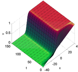
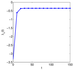
Fig. 7: Solution for $u_{0}$ in Example 1 (left) and evolution of $\lambda_{v}$ (right) for $J=40$ and $\Delta x=0.1$.

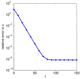
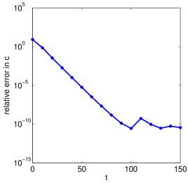
Fig. 8: Error in the approximation of $c$ for Example 1. Left: $\Delta x=0.1$, Right: $\Delta x=0.025$.

Example 2.

We consider the initial data

$$u_{0}(x)=\frac{1}{2}\Big{(}1+0.53\frac{x}{J}+0.47\sin\Big{(}-\frac{3\pi x}{2J}\Big{)}\Big{)}.$$ (90)

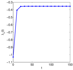
Fig. 9: Solution for $u_{0}$ in Example 2(left) and evolution of $\lambda_{v}$ (right) for $J=40$ and $\Delta x=0.1$.

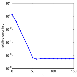
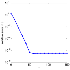
Fig. 10: Error in the approximation of $c$ for Example 2. Left: $\Delta x=0.1$, Right: $\Delta x=0.025$.

Example 3.

We consider the initial data

$$u_{0}(x)=\left\{\begin{array}[]{ll}0.2,&\mbox{if }\ x<0\\ 0.8,&\mbox{if }\ x>0.\end{array}\right.$$ (91)

In this case $u_{0}$ does not satisfy the boundary conditions. We chose this example because if we consider the natural extension of $u_{0}$ to the whole line (by 0.8 to the right and 0.2 to the left), Theorem 7 guarantees the convergence of the solution of (84) to $\Phi$ in (85).

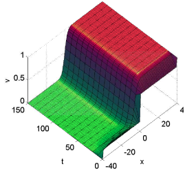
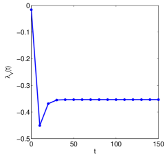
Fig. 11: Solution for $u_{0}$ in Example 2 (left) and evolution of $\lambda_{v}$ (right) for $J=40$ and $\Delta x=0.1$.

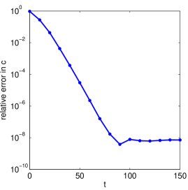
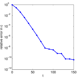
Fig. 12: Error in the approximation of $c$ for Example 2. Left: $\Delta x=0.1$, Right: $\Delta x=0.025$.

Appendix A Technical lemma

We include in this appendix a technical result, where we study in detail the behavior at $\pm\infty$ of the bounded solutions to a certain kind of second order differential equations with variable coefficients.

Lemma 32.

Let $c\in\mathbb{R}$ and let us consider the second order (non homogeneous) scalar differential equation

$$\psi^{\prime\prime}(x)+c\psi^{\prime}(x)+a(x)\psi(x)=f(x),\qquad x_{0}<x<\infty,$$ (92)

where

i) $a(x)$ is a bounded piecewise continuous function satisfying

$$\limsup_{x\to+\infty}|a(x)-a|\leq M_{1}e^{-\theta x},$$ (93)

ii) the function $f(x)$ satisfies

$$|f(x)|\leq M_{2}e^{-\tau x},$$ (94)

where $\theta,\tau>0$. Then any bounded solution $\psi$ of (92) tends to 0 as $x\to\infty$. Moreover, if $0<\omega<\min\{\theta,-r_{1},\tau\}$, with $r_{1}=\frac{-c-\sqrt{c^{2}-4a}}{2}<0$, then

$$|\psi(x)|,\,|\psi^{\prime}(x)|,\,|\psi^{\prime\prime}(x)|\leq Me^{-\omega x},\quad\mbox{ for }\ x\geq x_{2},$$

for some constant $M>0$.

Proof.

Let us rewrite the equation 92 as

$$\psi^{\prime\prime}+c\psi^{\prime}+a\psi=(a-a(x))\psi(x)+f(x):=b(x),$$ (95)

and observe that from i) and ii) we have $|b(x)|\leq Me^{-\gamma x}$ for some $M>0$ and with $\gamma=\min\{\tau,\theta\}>0$.

The roots of the characteristic equation associated to the homogeneous equation of (95) are precisely

$$r_{1}=\frac{-c-\sqrt{c^{2}-4a}}{2}<0\qquad\mbox{ and }\qquad r_{2}=\frac{-c+\sqrt{c^{2}-4a}}{2}>0.$$ (96)

By the variation of constants formula, any solution $\psi$ of (95) is of the form

$$\psi(x)=Ce^{r_{1}x}+De^{r_{2}x}+\frac{1}{r_{1}-r_{2}}\int_{x_{0}}^{x}(e^{r_{1}(x-s)}-e^{r_{2}(x-s)})b(s)\,ds,$$ (97)

for $C,D\in\mathbb{R}$. If require further that $\psi$ is bounded, the only possible choice for $D$ is

$$D=\frac{1}{r_{1}-r_{2}}\int_{x_{0}}^{\infty}e^{-r_{2}s}b(s)\,ds,$$ (98)

leading to

$$\psi(x)=Ce^{r_{1}x}+\frac{e^{r_{1}x}}{r_{1}-r_{2}}\int_{x_{0}}^{x}e^{-r_{1}s}b(s)\,ds+\frac{e^{r_{2}x}}{r_{1}-r_{2}}\int_{x}^{\infty}e^{-r_{2}s}b(s)\,ds.$$ (99)

But, if $r_{1}+\gamma\neq 0$, then

$$\left|\int_{x_{0}}^{x}e^{-r_{1}s}b(s)\,ds\right|\leq M\int_{x_{0}}^{x}e^{-(r_{1}+\gamma)s}\leq M\frac{e^{-(r_{1}+\gamma)x_{0}}-e^{-(r_{1}+\gamma)x}}{r_{1}+\gamma}$$

and if $r_{1}+\gamma=0$, then

$$\left|\int_{x_{0}}^{x}e^{-r_{1}s}b(s)\,ds\right|\leq M(x-x_{0}).$$

Moreover, since $r_{2}+\gamma>0$, we have

$$\left|\int_{x}^{\infty}e^{-r_{2}s}b(s)\,ds\right|\leq M\int_{x}^{\infty}e^{-(r_{2}+\gamma)s}\leq M\frac{e^{-(r_{2}+\gamma)x}}{r_{2}+\gamma}.$$

Plugging these estimates in (99), and with some simple computations we obtain that, if $r_{1}+\gamma\neq 0$ then

$$|\psi(x)|\leq C_{1}e^{r_{1}x}+C_{2}e^{-\gamma x}+C_{3}e^{-\gamma x}$$

and if $r_{1}+\gamma=0$, then

$$|\psi(x)|\leq C_{1}e^{r_{1}x}+C_{2}e^{-\gamma x}(x-x_{0})+C_{3}e^{-\gamma x},$$

from where the conclusion for $\psi$ follows easily.

To obtain the bounds for $\psi^{\prime}(x)$ we just take derivatives in (99). We obtain an extra term, $b(x)$, and the rest of the terms are estimated similarly as in the case of $\psi(x)$. To estimate $\psi^{\prime\prime}(x)$ we use the equation satisfied by $\psi$ and the bounds obtained for $\psi(x)$ and $\psi^{\prime}(x)$. ∎

Remark 10.

The same conclusions of the previous Lemma hold if we are dealing with the interval $-\infty<x<x_{1}$. In this case we need to specify the behavior of the functions $a(\cdot)$ and $f(\cdot)$ as $x\to-\infty$ and the conclusion is the exponential decay of the solution as $x\to-\infty$.

Appendix B Proof of Lemma 73

Finally, we include in this appendix a proof of Lemma 27.

Proof.

$(i)$ and $(ii)$ follow from [19, Section 5.4 and Appendix A].

$(iii)$ Observe first that we know the behavior of $\Phi_{\infty}(x),\Phi^{\prime}_{\infty}(x)$ as $x\to\pm\infty$. Notice that the orbit $x\to(\Phi_{\infty}(x),\Phi^{\prime}_{\infty}(x))$ is the heteroclinic orbit connecting $(0,0)$ (as $x\to-\infty$) with $(1,0)$ (as $x\to+\infty$) of the ODE,

$$\left\{\begin{array}[]{l}U^{\prime}=V,\\ V^{\prime}=-\lambda V-f(U)\end{array}\right.$$ (100)

and therefore the orbit lies in the unstable manifold of $(0,0)$ and the stable manifold of $(1,0)$. Via linearization of the equation in $(0,0)$ and $(1,0)$ we can obtain that if we define

$$r_{1}=\frac{-\lambda-\sqrt{\lambda^{2}-4f^{\prime}(1)}}{2},\qquad r_{2}=\frac{-\lambda+\sqrt{\lambda^{2}-4f^{\prime}(0)}}{2},$$

we have

$$|\Phi_{\infty}(x)|,|\Phi^{\prime}_{\infty}(x)|\leq Ce^{r_{2}x},\hbox{ as }x\to-\infty,$$

$$|\Phi_{\infty}(x)-1|,|\Phi^{\prime}_{\infty}(x)|\leq Ce^{r_{1}x},\hbox{ as }x\to+\infty$$

and therefore

$$|f(\Phi_{\infty})|,|f^{\prime}(\Phi_{\infty}(x))-f^{\prime}(0)|\leq Ce^{r_{2}x},\hbox{ as }x\to-\infty$$

and

$$|f(\Phi_{\infty})|,|f(\Phi^{\prime}_{\infty}(x))-f^{\prime}(1)|\leq Ce^{r_{1}x},\hbox{ as }x\to+\infty.$$

Using the equation for $\Phi_{\infty}$, that is, $\Phi_{\infty}^{\prime\prime}=-\lambda\Phi^{\prime}_{\infty}-f(\Phi_{\infty})=0$, we get also

$$|\Phi^{\prime\prime}_{\infty}(x)|\leq Ce^{r_{2}x},\hbox{ as }x\to-\infty,\quad|\Phi^{\prime\prime}_{\infty}(x)|\leq Ce^{r_{1}x},\hbox{ as }x\to+\infty.$$

Applying Lemma 32 and Remark 10, we have that if there exists a function $w$ such that $L_{0}^{\infty}w=\Phi^{\prime}_{\infty}$, then

$$|w(x)|,|w^{\prime}(x)|,|w^{\prime\prime}(x)|\leq Ce^{r_{2}^{-}x},\hbox{ as }x\to-\infty,$$

and

$$|w(x)|,|w^{\prime}(x)|,|w^{\prime\prime}(x)|\leq Ce^{r_{1}^{-}x},\hbox{ as }x\to+\infty.$$

where $0<r_{2}^{-}<r_{2}$ and $r_{1}<r_{1}^{-}<0$ but arbitrarily close to $r_{2}$ and $r_{1}$, respectively.

Once this estimates have been obtained, we can perform the change of variables $v(x)=e^{\frac{\lambda}{2}x}w(x)$ which will be a function in $H^{2}(\mathbb{R})$, because of the estimates found above for $w,w^{\prime},w^{\prime\prime}$. Therefore, $v$ will be a solution of

$$v^{\prime\prime}+\left(f^{\prime}(\Phi_{\infty}(x))+\frac{|\lambda|^{2}}{2}\right)v=\chi_{\infty}(x),$$ (101)

where $\chi_{\infty}(x)=e^{\frac{\lambda}{2}x}\Phi^{\prime}_{\infty}(x)$, which is a function in $L^{2}(\mathbb{R})$ because of the exponential bounds obtained for $\Phi^{\prime}_{\infty}(x)$ and it is an eigenfunction of the operator $v\to v^{\prime\prime}+\left(f^{\prime}(\Phi(x))+\frac{|\lambda|^{2}}{2}\right)v$ associated to the eigenvalue $0$. But this operator is selfadjoint and therefore there cannot exist a solution of equation (101). ∎

References

- [1] D. G. Aronson, H. F. Weinberger, Multidimensional nonlinear diffusion arising in population genetics, Adv. Math., 30 (1978), pp. 33–76.
- [2] H. Berestycki, L. Nirenberg, S. R. S. Varadhan, The Principal Eigenvalue and Maximum Principles for Second-Order Elliptic Operators in General Domains, Comm. Pure Appl. Math., 47 (1994), pp. 47–92.
- [3] W. J. Beyn, J. Lorenz, Stability of traveling waves: dichotomies and eigenvalue conditions on finite intervals, Numer. Funct. Anal. Optim., 20 (1999), pp. 201-244.
- [4] W. J. Beyn, J. Rottman-Matthes, Resolvent estimates for boundary value problems on large intervals via the theory of discrete approximations, Numer. Funct. Anal. Optim., 28 (2007), pp. 603–629.
- [5] W. J. Beyn, V. Thümmler, Freezing solutions of equivariant evolution equations, SIAM J. Appl. Dyn. Syst., 3 (2004), pp. 85–116.
- [6] W. J. Beyn, V. Thümmler, Phase conditions, symmetries, and PDE continuation, Numerical continuation methods for dynamical systems, pp. 301–330, Underst. Complex Syst., Springer, Dordrecht, 2007.
- [7] T. Cazenave, A. Haraux, An introduction to semilinear evolution equations, Clarendon Press, Oxford, 1998.
- [8] W.A. Coppel Dichotomies in Stability theory, Lecture Notes in Mathematics, Vol. 629. Springer-Verlag, Berlin-New York, (1978)
- [9] F.A. Davidson, N. Dodds, Spectral properties of non-local differential operators, Appl. Anal., 85 (2006), pp. 717–734.
- [10] F.A. Davidson, N. Dodds, Spectral properties of non-local uniformly-elliptic operators, Electron. J. Differential Equations, 126 (2006), 15 pp.
- [11] N. Dodds, Further spectral properties of uniformly elliptic operators that include a non-local term, Appl. Math. Comput., 197 (2008), pp. 317- 327.
- [12] B. Fiedler, P. Polacik, Complicated dynamics of scalar reaction diffusion equations with a nonlocal term, Proc. Roy. Soc. Edinburgh Sect. A, 115 (1990), pp. 167–192.
- [13] P. C. Fife, J. B. McLeod, The approach of solutions of nonlinear diffusion equations to travelling front solutions, Arch. Rational Mech. Anal., 65 (1977), pp. 335–361.
- [14] P. Freitas, A nonlocal Sturm-Liouville eigenvalue problem, Proc. Roy. Soc. Edinburgh Sect. A, 124 (1994), pp. 169–188.
- [15] P. Freitas, Non-local reaction diffusion equations, Fields Institute Communications, 21 (1999), pp. 187–204.
- [16] A. Friedman, Partial differential equations of parabolic type, Prentice Hall, Inc., Englewood Cliffs, N.J. 1964.
- [17] E. Hairer, G. Wanner, Solving ordinary differential equations II. Stiff and Differential-Algebraic Problems, 2nd ed., Springer Ser. Comput. Math. 14, Springer-Verlag, Berlin, 1996.
- [18] J. Hale, Ordinary differential equations. 2nd ed., Robert E. Krieger Publishing Co., Inc., Huntington, New York, 1980.
- [19] D. Henry, Geometric theory of semilinear parabolic equations, Lecture Notes in Mathematics 840, Springer, Berlin, 1981.
- [20] T. Kato, Schrödinger operators with singular potentials, Israel J. Math., 13 (1972), pp. 135–148.
- [21] T. Kato, Perturbation theory for linear operators, Springer-Verlag, New York-Berlin, 1982.
- [22] K. Palmer Exponential dichotomies and transversal homoclinic points, J. Differential Equations, 55 (1984), pp. 225–256.
- [23] B. Sandstede, Stability of travelling waves, Handbook of dynamical systems, Vol. 2, 983–1055, North-Holland, Amsterdam, 2002.
- [24] H. Takase, B. D. Sleeman, Generalized travelling coordinate for systems of reaction-diffusion equations, IMA J. Appl. Math., 64 (2000), pp. 1–22.
- [25] V. Thümmler, Numerical analysis of the method of freezing travelling waves, Doctoral Thesis, Univ. Bielefeld, 2005.
- [26] V. Thümmler, The effect of freezing and discretization to the asymptotic stability of relative equilibria, J. Dynam. Differential Equations, 20 (2008), pp. 425–477.
- [27] V. Thümmler, Numerical Approximation of Relative Equilibria for Equivariant PDEs, SIAM J. Numer. Anal., 46 (2008), pp. 2978–3005.
- [28] A. I. Volpert, V. A. Volpert, V. A. Volpert, Traveling wave solutions of parabolic systems. Translations of Mathematical Monographs, 140. American Mathematical Society, Providence, RI, 1994.
- [29] G. Vainikko, Funktionalanalysis der Diskretisierungsmethoden, Leipzig 1976.
- [30] G. Vainikko, Über die Konvergenz und Divergenz von Näherungsmethoden bei Eigenwertproblemen, Math. Nachr. 78 (1977), pp. 145–164.
- [31] G. Vainikko, Regular convergence of operators and the approximate solution of equations, Mathematical Analysis, Vol. 16 (Russian), 5- 53, 151, VINITI, Moscow, 1979.