Statistical Mechanics and the Physics of the Many-Particle Model Systems

The development of methods of quantum statistical mechanics is considered in light of their applications to quantum solid-state theory. We discuss fundamental problems of the physics of magnetic materials and the methods of the quantum theory of magnetism, including the method of two-time temperature Green’s functions, which is widely used in various physical problems of many-particle systems with interaction. Quantum cooperative effects and quasiparticle dynamics in the basic microscopic models of quantum theory of magnetism: the Heisenberg model, the Hubbard model, the Anderson Model, and the spin-fermion model are considered in the framework of novel self-consistent-field approximation. We present a comparative analysis of these models; in particular, we compare their applicability for description of complex magnetic materials. The concepts of broken symmetry, quantum protectorate, and quasiaverages are analyzed in the context of quantum theory of magnetism and theory of superconductivity. The notion of broken symmetry is presented within the nonequilibrium statistical operator approach developed by D.N. Zubarev. In the framework of the latter approach we discuss the derivation of kinetic equations for a system in a thermal bath. Finally, the results of investigation of the dynamic behavior of a particle in an environment, taking into account dissipative effects, are presented.

Keywords: Quantum statistical physics; quantum theory of magnetism; theory of superconductivity; Green’s function method; Hubbard model and other many-particle models on a lattice; symmetry principles; breaking of symmetries; Bogoliubov’s quasiaverages; quasiparticle many-body dynamics; magnetic polaron; microscopic theory of the antiferromagnetism.

PACS: 05.30.-d, 05.30.Fk, 74.20.-z, 75.10.-b

1 Introduction

The purpose of this review is to trace the development of some methods of quantum statistical mechanics formulated by N.N. Bogoliubov, and also to show their effectiveness in applications to problems of quantum solid-state theory, and especially to problems of quantum theory of magnetism. It is necessary to stress, that the path to understanding the foundations of the modern statistical mechanics and the development of efficient methods for computing different physical characteristics of many-particle systems was quite complex. The main postulates of the modern statistical mechanics were formulated in the papers by J.P. Joule (1818-1889), R. Clausius (1822-1888), W. Thomson (1824-1907), J.C. Maxwell (1831-1879), L. Boltzmann (1844-1906), and, especially, by J.W. Gibbs (1839-1903). The monograph by Gibbs ”Elementary Principles in Statistical Mechanics Developed with Special Reference to the Rational Foundations of Thermodynamics” [1, 2] remains one of the highest peaks of modern theoretical science. A significant contribution to the development of modern methods of equilibrium and nonequilibrium statistical mechanics was made by Academician N.N. Bogoliubov (1909-1992) [3, 4, 5, 6, 7].
Specialists in theoretical physics, as well as experimentalists, must be able to find their way through theoretical problems of the modern physics of many-particle systems because of the following reasons. Firstly, the statistical mechanics is filled with concepts, which widen the physical horizon and general world outlook. Secondly, statistical mechanics and, especially, quantum statistical mechanics demonstrate remarkable efficiency and predictive ability achieved by constructing and applying fairly simple (and at times even crude) many-particle models. Quite surprisingly, these simplified models allow one to describe a wide diversity of real substances, materials, and the most nontrivial many-particle systems, such as quark-gluon plasma, the DNA molecule, and interstellar matter. In systems of many interacting particles an important role is played by the so-called correlation effects [8], which determine specific features in the behavior of most diverse objects, from cosmic systems to atomic nuclei. This is especially true in the case of solid-state physics. Investigation of systems with strong inter-electron correlations, complicated character of quasiparticle states, and strong potential scattering is an extremely important and topical problem of the modern theory of condensed matter. Our time is marked by a rapid advancement in design and application of new materials, which not only find a wide range of applications in different areas of engineering, but they are also connected with the most fundamental problems in physics, physical chemistry, molecular biology, and other branches of science. The quantum cooperative effects, such as magnetism and superconductivity, frequently determine the unusual properties of these new materials. The same can be also said about other non-trivial quantum effects like, for instance, the quantum Hall effect, the Bose-Einstein condensation, quantum tunneling and others. This research direction is developing very rapidly, setting a fast pace for widening the domain where the methods of quantum statistical mechanics are applied. This review will support the above statement by concrete examples.

2 Quantum Statistical Mechanics and Solid State Physics

The development of experimental techniques over the recent years opened the possibility for synthesis and investigations of a wide class of new substances with unusual combination of properties [9, 10, 11, 12, 13, 14, 15]. Transition and rare-earth metals and especially compounds containing transition and rare-earth elements possess a fairly diverse range of properties. Among those, one can mention magnetically ordered crystals, superconductors, compounds with variable valence and heavy fermions, as well as substances which under certain conditions undergo a metal-insulator transition, like perovskite-type manganites, which possesses a large magneto-resistance with a negative sign. These properties find widest applications in engineering; therefore, investigations of this class of substances should be classified as the currently most important problems in the physics of condensed matter. A comprehensive description of materials and their properties (as well as efficient predictions of properties of new materials) is possible only in those cases, when there is an adequate quantum-statistical theory based on the information about the electron and crystalline structures. The main theoretical problem of this direction of research, which is the essence of the quantum theory of magnetism [16, 17], is investigations and improvements of quantum-statistical models describing the behavior of the above-mentioned compounds in order to take into account the main features of their electronic structure, namely, their dual ”band-atomic” nature [18, 19]. The construction of a consistent theory explaining the electronic structure of these substances encounters serious difficulties when trying to describe the collectivization- localization duality in the behavior of electrons. This problem appears to be extremely important, since its solution gives us a key to understanding magnetic, electronic, and other properties of this diverse group of substances. The author of the present review investigated the suitability of the basic models with strong electron correlations and with a complex spectrum for an adequate and correct description of the dual character of electron states. A universal mathematical formalism was developed for this investigation [20]. It takes into account the main features of the electronic structure and allows one to describe the true quasiparticle spectrum, as well as the appearance of the magnetically ordered, superconducting, and dielectric (or semiconducting) states. With a few exceptions, diverse physical phenomena observed in compounds and alloys of transition and rare-earth metals [18, 19, 21], cannot be explained in the framework of the mean-field approximation, which overestimates the role of inter-electron correlations in computations of their static and dynamic characteristics. The circle of questions without a precise and definitive answer, so far, includes such extremely important (not only from a theoretical, but also from a practical point of view) problems as the adequate description of quasiparticle dynamics for quantum-statistical models in a wide range of their parameter values. The source of difficulties here lies not only in the complexity of calculations of certain dynamic properties (such as, the density of states, electrical conductivity, susceptibility, electron-phonon spectral function, the inelastic scattering cross section for slow neutrons), but also in the absence of a well-developed method for a consistent quantum-statistical analysis of a many-particle interaction in such systems. A self-consistent field approach was used in the papers [20, 22, 23, 24, 25, 26, 27] for description of various dynamic characteristics of strongly correlated electronic systems. It allows one to consistently and quite compactly compute quasiparticle spectra for many-particle systems with strong interaction taking into account damping effects. The correlation effects and quasiparticle damping are the determining factors in analysis of the normal properties of high-temperature superconductors, and of the transition mechanism into the superconducting phase. We also formulated a general scheme for a theoretical description of electronic properties of many-particle systems taking into account strong inter-electron correlations [20, 22, 23, 24, 26, 27]. The scheme is a synthesis of the method of two-time temperature Green’s functions [16] and the diagram technique. An important feature of this approach is a clear-cut separation of the elastic and inelastic scattering processes in many-particle systems (which is a highly nontrivial task for strongly correlated systems). As a result, one can construct a correct basic approximation in terms of generalized mean fields (the elastic scattering corrections), which allows one to describe magnetically ordered or superconducting states of the system. The residual correlation effects, which are the source of quasiparticle damping, are described in terms of the Dyson equation with a formally exact representation for the mass operator. There is a general agreement that for heavy-fermion compounds, the model Hamiltonian is well established (the periodic Anderson model or the periodic Kondo lattice), and the main theoretical challenge in this case lies in constructing accurate approximations. However, in the case of high-temperature superconductors or perovskite-type manganites, neither a model, nor adequate approximate analytical methods for its solution are available. Thus, the development and improvement of the methods of quantum statistical mechanics still remains quite an important direction of research [28].

3 Magnetic Properties of Substances and Models of Magnetic Materials

It is widely accepted that the appearance of magnetically ordered states in transition metals is to some extent a consequence of the atom-like character of $d$-states, but mostly it is the result of interatomic exchange interactions. In order to better understand the origin of quantum models of magnetic materials, we discuss here briefly the physical aspects of the magnetic properties of solid materials. The magnetic properties of substances belong to the class of natural phenomena, which were noticed a long time ago [17, 29]. Although it is assumed that we encounter magnetic natural phenomena less frequently than the electric ones, nevertheless as was noticed by V. Weisskopf, ”magnetism is a striking phenomenon; when we hold a magnet in one hand and a piece of iron in another, we feel a peculiar force, some ”force of nature”, similar to the force of gravity” [30]. It is interesting to note that the experiment-based scientific approach began from investigations of magnetic materials. This is the so called inductive method, which insists on searching for truth about the nature not in deductions, not in syllogisms and formal logics, but in experiments with the natural substances themselves. This method was applied for the first time by William Gilbert (1544-1603), Queen Elizabeth’s physician. In his book, ”On the magnet, magnetic bodies, and on the great magnet, the Earth” [31], published in 1600, he described over 600 specially performed experiments with magnetic materials, which had led him to an extremely important and unexpected for the time conclusion, that the Earth is a giant spherical magnet. Investigations of Earth’s and other planet’s magnetism is still an interesting and quite important problem of modern science [32, 33, 34]. Thus, it is with investigations of the physics of magnetic phenomena, that the modern experiment based science began. Note, that although the creation of the modern scientific methods is often attributed to Francis Bacon, Gilbert’s book appeared 20 years earlier than ”The New Organon” by Francis Bacon (1561-1626).
The key to understanding the nature of magnetism became the discovery of a close connection between magnetism and electricity [35]. For a long time the understanding of magnetism’s nature was based on the hypothesis of how the magnetic force is created by magnets. Andre Ampere (1775-1836) conjectured that the principle behind the operation of an ordinary steel magnet should be similar to an electric current passing over a circular or spiral wire. The essence of his hypothesis laid in the assumption, that each atom contains a weak circular current, and if most of these atomic currents are oriented in the same direction, then the magnetic force appears. All subsequent developments of the theory of magnetism consisted in the development and refinement of Ampere’s molecular currents hypothesis.
As an extension of this idea by Ampere a conjecture was put forward that a magnet is an ensemble of elementary double poles, magnetic dipoles. The dipoles have two magnetic poles which are inseparably linked. In 1907, Pierre Weiss (1865-1940) proposed a phenomenological picture of the magnetically ordered state of matter. He was the first to perform a phenomenological quantitative analysis of the magnetic phenomena in substances [36]. Weiss’s investigations were based on the notion, introduced by him, of a molecular field. Subsequently this approach was named the molecular (or mean, or effective) field approximation, and it is still being widely used even at the present time [37]. The simplest microscopic model of a ferromagnet in the molecular field’s approximation is based on the assumption that electrons form a free gas of magnetic arrows (magnetic dipoles), which imitate Ampere’s molecular currents. In the simplest case it is assumed that these ”elementary magnets” could orient in space either along a particular direction, or against it. In order to find the thermodynamically equilibrium value of the magnetization $\langle M\rangle$ as a function of temperature $T$, one has to turn to general laws of thermodynamics. This is especially important when we consider the behavior of a system at finite temperatures. Finding the equilibrium magnetization of a ferromagnet becomes quite a simple task if we first succeed in writing down its energy $E(\langle M\rangle)$ as a function of magnetization. All we have to do after that is to minimize the free energy $F(\langle M\rangle),$ which is defined by the following relationship [35]:

$$F(\langle M\rangle)=E(\langle M\rangle)-TS(\langle M\rangle).$$ (3.1)

Here, $S(\langle M\rangle)$ is the system entropy also written down as a function of magnetization. It is important to stress, that the problem of calculating the system entropy cannot be solved in the framework of just thermodynamics. In order to find the entropy one has to turn to statistical mechanics [1, 38, 39, 40, 41], which provides a microscopic foundation to the laws of thermodynamics. Note that derivations of equilibrium magnetization $\langle M\rangle$ as a function of temperature $T$, or, more generally, investigations of relationships between the free energy and the order parameter in magnetics and pyroelectrics are still ongoing even at the present time [42, 43, 44, 45]. Of course, modern investigations take into account all the previously accumulated experience. In the framework of the P. Weiss approach one investigates the appearance of a spontaneous magnetization $\langle M\rangle\neq 0$ for $H=0.$ This approach is based on the following postulate for the behavior of the system’s energy

$$E(\langle M\rangle)\simeq NI(\langle M\rangle)^{2}.$$ (3.2)

This expression takes into account the interaction between elementary magnets (arrows). Here, $I$ is the energy of the Weiss molecular field per atomic magnetic arrow. The question on the microscopic nature of this field is beyond the framework of the Weiss approach. The minimization of the free energy $F(\langle M\rangle)$ yields the following relationship

$$\langle M\rangle=th(T_{C}\langle M\rangle/T),$$ (3.3)

Where $T_{C}$ is the Curie or the critical temperature. As the temperature decreases below this critical value a spontaneous magnetization appears in the system. The Curie temperature was named in honor of Pierre Curie (1859-1906), who established the following law for the behavior of susceptibility $\chi$ in paramagnetic substances

$$\chi=\lim_{H\rightarrow 0}\frac{\langle M\rangle}{H}=\frac{C}{T}.$$ (3.4)

Depending on the actual material, the Curie parameter $C$ obtains different (positive) values [35]. Note that Pierre Curie performed thorough investigations of the magnetic properties of iron back in 1895. In the process of those experiments he established the existence of a critical temperature for iron, above which the ferromagnetic properties disappear. These investigations laid a foundation for investigations of order-disorder phase transitions, and other phase transformations in gases, liquids, and solid substances. This research direction created the core of the physics of critical phenomena, which studies the behavior of substances in the vicinity of critical temperatures [46].
Extensive investigations of spontaneous magnetization and other thermal effects in nickel in the vicinity of the Curie temperature were performed by Weiss and his collaborators [47]. They developed a technique for measuring the behavior of the spontaneous magnetization in experimental samples for different values of temperature. Knowing the behavior of spontaneous magnetization as a function of temperature one can determine the character of magnetic transformations in the material under investigation. Investigations of the behavior of the magnetic susceptibility as a function of temperature in various substances remain important even at the present time [48, 49, 50].
Within the P. Weiss approach we obtain the following expression for the Curie temperature

$$T_{C}=2I/k_{B}.$$ (3.5)

In order to obtain a rough estimate for the magnitude of $I$ take $T_{C}=1000\,\textrm{K}.$ Then one obtains $I\sim 10^{-13}$ erg/atom. This implies that the only origin of the Weiss molecular field can be the Coulomb interaction of electrical charges [16, 35]. Computations in the framework of the molecular field method lead to the following formula for the magnetic susceptibility

$$\chi=N\mu_{B}^{2}\langle M\rangle/H=\frac{N\mu_{B}^{2}}{k_{B}(T-T_{C})},$$ (3.6)

where $\mu_{B}=e\hbar/2mc$ is the Bohr magneton (within the Weiss approach this is the magnetic moment of the magnetic arrows imitating Ampere’s molecular currents). The above expression for the susceptibility is referred to as the Curie-Weiss law. Thus, the Weiss molecular field, whose magnitude is proportional to the magnetization, is given by

$$H_{W}=k_{B}T_{C}\langle M\rangle/\mu_{B}.$$ (3.7)

Researchers tried to find the answer to the question on the nature of this internal molecular field in ferromagnets for a long time. That is, they tried to figure out which interaction causes the parallel alignment of electron spins. As was stressed in the book [51]: ”At first researchers tried to imagine this interaction of electrons in a given atom with surrounding electrons as some quasi-magnetic molecular field, acting on the electrons of the given atom. This hypothesis served as a foundation for the P. Weiss theory, which allowed one to describe qualitatively the main properties of ferromagnets”. However, it was established that Weiss’s molecular field approximation is applicable neither for theoretical interpretation, nor for quantitative description of various phenomena taking place in the vicinity of the Curie temperature. Although numerous attempts aiming to improve Weiss’s mean-field theory were undertaken, none of them led to significant progress in this direction. Numerical estimates yield the value $H_{W}=10^{7}$ oersted for the magnitude of the Weiss mean field. The nonmagnetic nature of the Weiss molecular field was established by direct experiments in 1927 (see the books [35, 51]). Ya.G. Dorfman performed the following experiment. An electron beam passing though nickel foil magnetized to the saturation level is falling on a photographic plate. It was expected that if such a strong magnetic field indeed exists in nickel, then the electrons passing through the magnetized foil would deflect. However, it turned out that the observed electron deflection is extremely small. The experiment led to the conclusion that, contrary to the consequences of the Weiss theory, the internal fields of large intensity are not present in ferromagnets. Therefore, the spin ordering in ferromagnets is caused by forces of a nonmagnetic origin. It is interesting that fairly recently, in 2001, similar experiments were performed again [52] (in a substantially modified form, of course). A beam of polarized ”hot” electrons was scattered by thin ferromagnetic nickel, iron, and cobalt films, and the polarization of the scattered electrons was measured. The concept of the Weiss exchange field $\textbf{W}(x)\sim-J_{\alpha}\textbf{S}(x)$ was used for theoretical analysis [52, 53]. The real part of this field corresponds to the exchange interaction between the incoming electrons and the electron density of the film (the imaginary part is responsible for absorption processes). The derived equations, describing the beam scattering, resemble quite closely the corresponding equations for the Faraday’s rotation effect in the light passing through a magnetized environment [52, 53]. The theoretical consideration is based on using the mean-field approximation, namely on the replacement

$$\textbf{W}\simeq\langle\textbf{W}(x)\rangle=J_{\alpha}\langle\textbf{S}(x)\rangle.$$ (3.8)

The subsequent quite rigorous and detailed consideration [53] aimed at deriving the effective quantum dynamics of the field $W(x)$ showed, that this dynamics is described by the Landau-Lifshitz equation [35]. The spatial and temporal variations of the field $W(x)$ are described by spin waves. The quanta of the Weiss exchange field are magnons.
One has to note that in its original version, the Weiss molecular field was assumed to be uniformly distributed over the entire volume of the sample, and had the same magnitude in all points of the substance. An entirely different situation takes place in a special class of substances called antiferromagnets. As the temperature of antiferromagnets falls below a particular value, a magnetically ordered state appears in the form of two inserted into each other sublattices with opposite directions of the magnetization. This special value of the temperature became known as the Neel temperature, after the founder of the antiferromagnetism theory L. Neel (1904-2000). In order to explain the nature of the antiferromagnetism (as well as of the ferrimagnetism) L. Neel introduced a profound and nontrivial notion of local molecular fields [54]. However, there was no a unified approach to investigations of magnetic transformations in real substances. Moreover, a consistent consideration of various aspects of the physics of magnetic phenomena on the basis of quantum mechanics and statistical physics was and still is an exceptionally difficult task, which to the present days does not have a complete solution [55, 56]. This was the reason why the authors of the most complete, at that time, monograph on the magnetism characterized the state of affairs in the physics of magnetic phenomena as follows: ”Even recently the problems of magnetism seemed to belong to an exceptionally unrewarding area for theoretical investigations. Such a situation could be explained by the fact that the attention of researchers was devoted mostly to ferromagnetic phenomena, because they played and still play quite an important role in engineering. However, the theoretical interpretation of the ferromagnetism presents such formidable difficulties, that to the present day this area remains one of the darkest spots in the entire domain of physics” [57]. The magnetic properties and the structure of matter turned out to be interconnected subjects. Therefore, a systematic quantum-mechanical examination of the problem of magnetic substances was considered by most researchers [51, 58, 59, 60] as quite an important task. Heisenberg, Dirac, Hund, Pauli, van Vleck, Slater, and many other researchers contributed to the development of the quantum theory of magnetism. As was noted by D. Mattis [17], ”…by 1930, after four years of most exciting and striking discoveries in the history of theoretical physics, a foundation for the modern electron theory of matter was laid down, after that an epoch of consolidation and computations had began, which continues up to the present day”.
Over the last decades the physics of magnetic phenomena became a vast and ramified domain of modern physical science [17, 35, 55, 56, 61, 62, 63, 64, 65, 66, 67, 68, 69, 70, 71, 72, 73, 74]. The rapid development of the physics of magnetic materials was influenced by introduction and development of new physical methods for investigating the structural and dynamical properties of magnetic substances [75]. These methods include magnetic neutron diffraction analysis [76, 77], NMR and EPR-spectroscopy, the Mossbauer effect, novel optical methods [78], as well as recent applications of synchrotron radiation [79, 80, 81, 82]. In particular, unique possibilities of the thermal neutron’s scattering methods [75, 76, 77, 83] allow one to obtain information on the magnetic and crystalline structure of substances, on the distribution of magnetic moments, on the spectrum of magnetic excitations, on critical fluctuations, and on many other properties of magnetic materials. In order to interpret the data obtained via inelastic scattering of slow neutrons one has to take into account electron-electron and electron-nuclear interactions in the system, as well as the Pauli exclusion principle. Here, we again face the challenge of considering various aspects of the physics of magnetic phenomena, consistently on the basis of quantum mechanics and statistical physics. In other words, we are dealing with constructing a consistent quantum theory of magnetic substances. As was rightly noticed by K. Yosida, ”The question of electron correlations in complex electronic systems is the beginning and the end of all research on magnetism” [84]. Thus, the phenomena of magnetism can be described and interpreted consistently only in the framework of quantum statistical theory of many interacting particles.

4 Quantum Theory of Magnetism

It is well known that ”quantum mechanics is the key to understanding magnetism” [85]. One of the first steps in this direction was the formulation of ”Hund’s rules” in atomic physics [63]. As was noticed by D. Mattis [17], ”The accumulated spectroscopic data allowed Stoner (1899-1968) to attribute the correct number of equivalent electrons to each atomic shell, and Hund (1896-1997) to state his rules, related to the spontaneous magnetic moments of a free atom or ion”. Hund’s rules are empirical recipes. Their consistent derivation is a difficult task. These rules are stated as follows:
(1) The ground state of an atom or an ion with a $L-S$ coupling is a state with the maximal multiplicity $(2S+1)$ for a given electron configuration.
(2) From all possible states with the maximal multiplicity, the ground state is a state with the maximal value of $L$ allowed by the Pauli exclusion principle.
Note that the applicability of these empirical rules is not restricted to the case, when all electrons lie in a single unfilled valency shell. A rigorous derivation of Hund’s rules is still missing. However, there are a few particular cases which show their validity under certain restrictions [63, 86] (see a recent detailed analysis of this question in the papers [87, 88]). Nevertheless Hund’s rules are very useful and are widely used for analysis of various magnetic phenomena. A physical analysis of the first Hund’s rule leads us to the conclusion, that it is based on the fact, that the elements of the diagonal matrix of the electron-electron’s Coulomb interaction contain the exchange’s interaction terms, which are entirely negative. This is the case only for electrons with parallel spins. Therefore, the more electrons with parallel spins involved, the greater the negative contribution of the exchange to the diagonal elements of the energy matrix. Thus, the first Hund’s rule implies that electrons with parallel spins ”tend to avoid each other” spatially. Here, we have a direct connection between Hund’s rules and the Pauli exclusion principle.
One can say that the Pauli exclusion principle (1925) lies in the foundation of the quantum theory of magnetic phenomena. Although this principle is merely an empirical rule, it has deep and important implications [89]. W. Pauli (1900-1958) was puzzled by the results of the ortho-helium terms analysis, namely, by the absence in the term structure of the presumed ground state, that is the $(1^{3}S)$ level. This observation stimulated him to perform a general examination of atomic spectra, with the aim to find out, if certain terms are absent in other chemical elements and under other conditions as well. It turned out, that this was indeed the case. Moreover, the conducted analysis of term systems had shown that in all the instances of missing terms the entire sets of the quantum numbers were identical for some electrons. And vice versa, it turned out that terms always drop out in the cases when entire sets of quantum numbers are identical. This observation became the essence of the Pauli exclusion principle:
The sets of quantum numbers for two (or many) electrons are never identical; two sets of quantum numbers, which can be obtained from one another by permutations of two electrons, define the same state.
In the language of many-electron wave functions one has to consider permutations of spatial and spin coordinates of electrons $i$ and $j$ in the case when both the spin variables $\sigma_{i}=\sigma_{j}=\sigma_{0}$ and the spatial coordinates $\vec{r}_{i}=\vec{r}_{j}=\vec{r}_{0}$ of these two electrons are identical. Then, we obtain:

$$P_{ij}\psi(\vec{r}_{1}\sigma_{1},\ldots\vec{r}_{i}\sigma_{i},\ldots\vec{r}_{j}\sigma_{j},\ldots)=\psi(\vec{r}_{1}\sigma_{1},\ldots\vec{r}_{i}\sigma_{i},\ldots\vec{r}_{j}\sigma_{j},\ldots).$$ (4.1)

The Pauli exclusion principle implies that

$$P_{ij}\psi(\vec{r}_{1}\sigma_{1},\ldots\vec{r}_{i}\sigma_{i},\ldots\vec{r}_{j}\sigma_{j},\ldots)=-\psi(\vec{r}_{1}\sigma_{1},\ldots\vec{r}_{i}\sigma_{i},\ldots\vec{r}_{j}\sigma_{j},\ldots).$$ (4.2)

The above conditions are satisfied simultaneously only in the case, when $\psi$ is equal to zero identically. Therefore, we arrive at the following conclusion: electrons are indistinguishable, that is, their permutations must not change observable properties of the system. The wave function changes or retains its sign under permutations of two particles depending on whether these indistinguishable particles are bosons or fermions. A consequence of the Pauli exclusion principle is the Aufbau principle, which leads to the periodicity in the properties of chemical elements. The fact that not more than one electron can occupy any single state leads also to such fundamental consequences as the very existence of solid bodies in nature. If the Pauli exclusion principle was not satisfied, no substance could ever be in a solid state. If the electrons would not have spin (that is, if they were bosons) all substances would occupy much smaller volumes (they would have higher densities), but they would not be rigid enough to have the properties of solid bodies.
Thus, the tendency of electrons with parallel spins ”to avoid each other” reduces the energy of electron-electron Coulomb interaction, and hence, lowers the system energy. This property has many important implications, in particular, the existence of magnetic substances. Due to the presence of an internal unfilled $nd$- or $nf$-shell, all free atoms of transition elements are strong magnetic, and this is a direct consequence of Hund’s rules. When crystals are formed [17, 35, 63, 68] the electronic shells in atoms reorganize, and in order to understand clearly the properties of crystalline substances, one has to know the wave function and the energies of (previously) outer-shell electrons. At the present time there are well-developed efficient methods for computing electronic energy levels in crystals [90, 91, 92]. Speaking qualitatively, we have to find out how the atomic wave’s functions change when crystals are formed, and how significantly they delocalize [19].

4.1 The Method of Model Hamiltonians

The method of model Hamiltonians proved to be very efficient in the theory of magnetism. Without any exaggeration one can say, that the tremendous successes in the physics of magnetic phenomena were achieved, largely, as a result of exploiting a few simple and schematic model concepts for ”the theoretical interpretation of ferromagnetism” [93]. One can regard the Ising model [94, 95] as the first model of the quantum theory of magnetism. In this model, formulated by W. Lenz (1888-1957) in 1920 and studied by E. Ising (1900-1998), it was assumed that the spins are arranged at the sites of a regular one-dimensional lattice. Each spin can obtain the values $\pm\hbar/2$:

$$\mathcal{H}=-\sum_{<ij>}I_{ij}S^{z}_{i}S^{z}_{j}.$$ (4.3)

This was one of the first attempts to describe the magnetism as a cooperative effect. It is interesting that the one-dimensional Ising model was solved by Ising in 1925, while the exact solution of the Ising model on a two-dimensional square lattice was obtained by L. Onsager (1903-1976) [96, 97] only in 1944. However, the Ising model oversimplifies the situation in real crystals. W. Heisenberg (1901-1976) [98] and P. Dirac (1902-1984) [99] formulated the Heisenberg model, describing the interaction between spins at different sites of a lattice by the following isotropic scalar function

$$\mathcal{H}=-\sum_{ij}J(i-j)\vec{S}_{i}\vec{S}_{j}-g\mu_{B}H\sum_{i}S_{i}^{z}.$$ (4.4)

Here $J(i-j)$ (the ”exchange integral”) is the strength of the exchange interaction between the spins located at the lattice sites $i$ and $j$. It is usually assumed that $J(i-j)=J(j-i)$ and $J(i-j=0)=0,$ which means that only the inter-site interaction is present (there is no self-interaction). The Heisenberg Hamiltonian (4.4) can be rewritten in the following form:

$$\mathcal{H}=-\sum_{ij}J(i-j)(S^{z}_{i}S^{z}_{j}+S^{+}_{i}S^{-}_{j}).$$ (4.5)

Here, $S^{\pm}=S^{x}\pm iS^{y}$ are the spin raising and lowering operators. They satisfy the following set of commutation relationships:

$$[S^{+}_{i},S^{-}_{j}]_{-}=2S^{z}_{i}\delta_{ij};\quad[S^{+}_{i},S^{-}_{i}]_{+}=2S(S+1)-2(S^{z}_{i})^{2};$$

$$[S^{\mp}_{i},S^{z}_{j}]_{-}=\pm S^{\mp}_{i}\delta_{ij};\quad S^{z}_{i}=S(S+1)-(S^{z}_{i})^{2}-S^{-}_{i}S^{+}_{i};$$

$$(S^{+}_{i})^{2S+1}=0,\quad(S^{-}_{i})^{2S+1}=0.$$

Note that in the isotropic Heisenberg model the $z$-component of the total spin $S^{z}_{tot}=\sum_{i}S^{z}_{i}$ is a constant of motion, that is $[H,S^{z}_{tot}]=0$.
Thus, in the framework of the Heisenberg-Dirac-van Vleck model [59, 98, 99, 100, 101], describing the interaction of localized spins, the necessary conditions for the existence of ferromagnetism involve the following two factors. Atoms of a ”ferromagnet to be” must have a magnetic moment, arising due to unfilled electron $d$- or $f$-shells. The exchange integral $J_{ij}$ related to the electron exchange between neighboring atoms must be positive. Upon fulfillment of these conditions the most energetically favorable configurations in the absence of an external magnetic field correspond to parallel alignment of magnetic moments of atoms in small areas of the sample (domains) [101]. Of course, this simplified picture is only schematic. A detail derivation of the Heisenberg-Dirac-van Vleck model describing the interaction of localized spins is quite complicated. Because of a shortage of space we cannot enter into discussion of this quite interesting topic [102, 103, 104]. An important point to keep in mind here is that magnetic properties of substances are born by quantum effects, the forces of exchange interaction [105].
As was already mentioned above, the states with antiparallel alignment of neighboring atomic magnetic moments are realized in a fairly wide class of substances. As a rule, these are various compounds of transition and rare-earth elements, where the exchange integral $J_{ij}$ for neighboring atoms is negative. Such a magnetically ordered state is called antiferromagnetism [54, 106, 107, 108, 109, 110, 111, 112, 113, 114, 115, 116]. In 1948, L. Neel introduced the notion of ferrimagnetism [117, 118, 119, 120, 121, 122] to describe the properties of substances in which spontaneous magnetization appears below a certain critical temperature due to nonparallel alignment of the atomic magnetic moment [123, 109, 110, 111, 112, 113, 114, 115, 116]. These substances differ from antiferromagnets where sublattice magnetizations $m_{A}$ and $m_{B}$ usually have identical absolute values, but opposite orientations. Therefore, the sublattice magnetizations compensate for each other and do not result in a macroscopically observable value for magnetization. In ferrimagnetics the magnetic atoms occupying the sites in sublattices $A$ and $B$ differ both in the type and in the number. Therefore, although the magnetizations in the sublattices $A$ and $B$ are antiparallel to each other, there exists a macroscopic overall spontaneous magnetization [109, 111, 112, 116, 118].
Later, substances possessing weak ferromagnetism were investigated [109, 110, 111, 112, 113, 114, 115, 116]. It is interesting that originally Neel used the term parasitic ferromagnetism [125] when referring to a small ferromagnetic moment, which was superimposed on a typical antiferromagnetic state of the $\alpha$ iron oxide $Fe_{2}O_{3}$ (hematite) [124]. Later, this phenomenon was called canted antiferromagnetism, or weak ferromagnetism [124, 126]. The weak ferromagnetism appears due to antisymmetric interaction between the spins $\vec{S}_{1}$ and $\vec{S}_{2}$ and which is proportional to the vector product $\vec{S}_{1}\times\vec{S}_{2}.$ This interaction is written in the following form

$$\mathcal{H}_{DM}\sim\vec{D}\vec{S}_{1}\times\vec{S}_{2}.$$ (4.6)

The interaction (4.6) is called the Dzyaloshinsky-Moriya interaction [127, 128]. Hematite is one of the most well known minerals [124, 126, 129, 130, 131], which is still being intensively studied [132] even at the present time [133, 134, 135, 136].
Thus, there exist a large number of substances and materials that possess different types of magnetic behavior: diamagnetism, paramagnetism, ferromagnetism, antiferromagnetism, ferrimagnetism, and weak ferromagnetism. We would like to note that the variety of magnetism is not exhausted by the above types of magnetic behavior; the complete list of magnetism types is substantially longer [137]. As was already stressed, many aspects of this behavior can be reasonably well described in the framework of a very crude Heisenberg-Dirac-van Vleck model of localized spins. This model, however, admits various modifications (see, for instance, the book [138]). Therefore, various nontrivial generalizations of the localized spin models were studied. In particular, a modification of the Heisenberg model was investigated, where, in addition to the exchange interaction between different sites, an exchange interaction between the spins at the same site was considered [139]:

$$\mathcal{H}=-\mu_{B}H\sum_{<i\alpha>}S^{z}_{i\alpha}-\frac{1}{2}\sum_{i\neq j}\sum_{\alpha\beta}J(i\alpha;j\beta)\left(\lambda S^{+}_{i\alpha}S^{-}_{j\beta}+S^{z}_{i\alpha}S^{z}_{j\beta}\right)-$$ (4.7)

$$\frac{1}{2}\sum_{i}\sum_{\alpha\neq\beta}J(i\alpha;i\beta)\left(\lambda S^{+}_{i\alpha}S^{-}_{i\beta}+S^{z}_{i\alpha}S^{z}_{i\beta}\right).$$

In the case when $J(i\alpha;i\beta)\gg J(i\alpha;j\beta)$, this model Hamiltonian in some sense imitates Hund’s rules. Indeed, Hund’s rules state that the triplet’s spin state of two electrons occupying one and the same site is energetically more favorable than the singlet state. It is this feature that is taken into account by the model (4.7). A model of this type was used for description of composite ferrites, which contain different types of atoms with different spins (magnetic moments). In the limiting case $J(i\alpha;i\beta)\neq 0;J(i\alpha;j\beta)\equiv 0$ the model (4.7) can be considered as the simplest version of the Heisenberg model [140]. In this case, the two-spin system is interpreted [140] as the simplest one-dimensional periodic magnet with the period $N=2$. Despite the apparent ’shortages’ model (4.7) has found numerous applications for description of real substances [141], including the composite $Cu(NO_{3})_{2}\cdot 2.5H_{2}O$-type salts [142, 143], of clusters [144, 145], as well as for improving mean-field approximation by using various cluster methods [146].

4.2 The Problem of Magnetism of Itinerant Electrons

The Heisenberg model describing localized spins is mostly applicable to substances where the ground state’s energy is separated from the energies of excited current-type states by a gap of a finite width. That is, the model is mostly applicable to semiconductors and dielectrics [111, 147]. However, the main strongly magnetic substances, nickel, iron, and cobalt, are metals, belonging to the transition group [35]. The development of quantum statistical theory of transition metals and of their compounds followed a more difficult path than that of the theory of simple metals [148, 149, 150, 151]. The traditional physical picture of the metal state was based on the notion of Bloch electron waves [148, 149, 150, 151, 152]. However, the role played by the inter-electron interaction remained unclear within the conventional approach. On the other hand, the development of the band theory of magnetism [62, 153, 154, 155, 156, 157], and investigations of the electronic phase’s transitions in transition and rare-earth metal compounds gradually led to realization of the determining role of electron correlations [158, 159, 160]. Moreover, in many cases inter-electron interaction is very strong and the description in terms of the conventional band theory is no longer applicable. Special properties of transition metals and of their alloys and compounds are largely determined by the dominant role of $d$-electrons. In contrast to simple metals, where one can apply the approximation of quasi-free electrons, the wave functions of $d$-electrons are much more localized, and, as a rule, have to be described by the tight-binding approximation [90, 91, 161]. The main aim of the band theory of magnetism and of related theories, describing phase ordering and phenomena of phase transition in complex compounds and oxides of transition and rare-earth metals, is to describe in the framework of a unified approach both the phenomena revealing the localized character of magnetically active electrons, and the phenomena where electrons behave as collectivized band entities [19]. A resolution of this apparent contradiction requires a very deep understanding of the relationship between the localized and the band description of electron states in transition and rare-earth metals, as well as in their alloys and compounds. The quantum statistical theory of systems with strong inter-electron correlations began to develop intensively when the main features of early semi-phenomenological theories were formulated in the language of simple model Hamiltonians. Both the Anderson model [162, 163], which formalized the Friedel theory of impurity levels, and the Hubbard model [164, 165, 166, 167, 168, 169], which formalized and developed early theories by Stoner, Mott, and Slater, equally stress the role of inter-electron correlations. The Hubbard Hamiltonian and the Anderson Hamiltonian (which can be considered as the local version of the Hubbard Hamiltonian) play an important role in the electron’s solid-state theory [20]. Therefore, as was noticed by E. Lieb [170], the Hubbard model is ’definitely the first candidate’ for constructing a ’more fundamental’ quantum theory of magnetic phenomena than the ’theory based on the Ising model’ [170] (see also the papers [171, 172, 173, 174, 175]).
However, as it turned out, the study of Hamiltonians describing strongly-correlated systems is an exceptionally difficult many-particle problem, which requires applications of various mathematical methods [170, 172, 173, 174, 175, 176, 177, 178]. In fact, with the exception of a few particular cases, even the ground state of the Hubbard model is still unknown. Calculation of the corresponding quasiparticle spectra in the case of strong inter-electron correlations also turned out to be quite a complicated problem. As was quite rightly pointed out by J. Kanamori [179], when one is dealing with ”a metal state with the values of parameters close to the critical point, where the metal turns into a dielectric”, then ”the calculation of excited states in such crystals becomes very difficult (especially at low temperatures)”. Therefore, in contrast to quantum many-body systems with weak interaction, the definition of such a notion as elementary excitations for strongly-interacting electrons with strong inter-electron correlations is quite a nontrivial problem requiring special detailed investigations [20, 22, 23, 24, 25, 26]. At the same time, one has to keep in mind, that the Anderson and Hubbard models were designed for applications to real systems, where both the case of strong and the case weak inter-electron correlations are realized.
Often, a very important role is played by the electron interaction with the lattice vibrations, the phonons [180, 181, 182]. Therefore, the number one necessity became the development of a systematic self-consistent theory of electron correlations applicable for a wide range of the parameter values of the main model, and the development of the electron-phonon’s interaction theory in the framework of a modified tight-binding approximation of strongly correlated electrons, as well as the examination of various limiting cases [183, 184]. All this activity allowed one to investigate the electric conductivity [185, 186], and the superconductivity [187, 188] in transition metals, and in their disordered alloys.

4.3 The Anderson and Hubbard Models

The Hamiltonian of the single-impurity Anderson model [26, 162, 163] is written in the following form:

$$\mathcal{H}=\sum_{k\sigma}\epsilon_{k}c^{{\dagger}}_{k\sigma}c_{k\sigma}+\sum_{\sigma}E_{0\sigma}f^{{\dagger}}_{0\sigma}f_{0\sigma}+U/2\sum_{\sigma}n_{0\sigma}n_{0-\sigma}+\sum_{k\sigma}V_{k}(c^{{\dagger}}_{k\sigma}f_{0\sigma}+f^{{\dagger}}_{0\sigma}c_{k\sigma}).$$ (4.8)

Here, $c^{{\dagger}}_{k\sigma}$ and $f^{{\dagger}}_{0\sigma}$ are the creation operators of conduction electrons and of localized impurity electrons, respectively, $\epsilon_{k}$ are the energies of conduction electrons, $E_{0\sigma}$ is the energy level of localized impurity electrons, and $U$ is the intra-atomic Coulomb interaction of the impurity-site electrons; $V_{k}$ is the $s-f$ hybridization. One can generalize the Hamiltonian of the single-impurity Anderson model to the periodic case:

$$\mathcal{H}=\sum_{k\sigma}\epsilon_{k}c^{{\dagger}}_{k\sigma}c_{k\sigma}+\sum_{i\sigma}E_{\sigma}f^{{\dagger}}_{i\sigma}f_{i\sigma}+U/2\sum_{i\sigma}n_{i\sigma}n_{i-\sigma}+\sum_{kj\sigma}V_{kj}(c^{{\dagger}}_{k\sigma}f_{j\sigma}+f^{{\dagger}}_{j\sigma}c_{k\sigma}).$$ (4.9)

The above Hamiltonian is called the periodic Anderson model. The Hamiltonian of the Hubbard model [164] is given by:

$$\mathcal{H}=\sum_{ij\sigma}t_{ij}a^{\dagger}_{i\sigma}a_{j\sigma}+U/2\sum_{i\sigma}n_{i\sigma}n_{i-\sigma}.$$ (4.10)

The above Hamiltonian includes the repulsion of the single-site intra-atomic Coulomb $U$, and $t_{ij}$, the one-electron hopping energy describing jumps from a $J$ site to an $i$ site. As a consequence of correlations electrons tend to ”avoid one another”. Their states are best modeled by atom-like Wannier wave functions $[\phi({\vec{r}}-{\vec{R}_{j}})]$. The Hubbard model’s Hamiltonian can be characterized by two main parameters: $U$, and the effective band width of tightly bound electrons

$$\Delta=(N^{-1}\sum_{ij}|t_{ij}|^{2})^{1/2}.$$

The band energy of Bloch electrons $\epsilon(\vec{k})$ is given by

$$\epsilon(\vec{k})=N^{-1}\sum_{\vec{k}}t_{ij}\exp[-i{\vec{k}}({\vec{R}_{i}}-{\vec{R}_{j}}],$$

where $N$ is the total number of lattice sites. Variations of the parameter $\gamma=\Delta/U$ allow one to study two interesting limiting cases, the band regime ($\gamma\gg 1$) and the atomic regime ($\gamma\rightarrow 0$). Note that the single-band Hubbard model (4.10) is a particular case of a more general model, which takes into account the degeneracy of $d$-electrons. In this case the second quantization is constructed with the aid of the Wannier functions of the form $[\phi_{\lambda}(r-R_{i})]$, where $\lambda$ is the band index ($\lambda$= 1,2,…5). The corresponding Hamiltonian of the electron system is given by

$$\mathcal{H}=\sum_{ij\mu\nu\sigma}t^{\mu\nu}_{ij}a^{{\dagger}}_{i\mu\sigma}a_{j\nu\sigma}+\frac{1}{2}\sum_{ij,mn}\sum_{\alpha\beta\gamma\delta\sigma\sigma^{\prime}}\langle i\alpha,j\beta|W|m\gamma,n\delta\rangle a^{{\dagger}}_{i\alpha\sigma}a^{{\dagger}}_{j\beta\sigma^{\prime}}a_{m\gamma\sigma^{\prime}}a_{n\delta\sigma}.$$ (4.11)

It can be rewritten in the following form

$$\mathcal{H}=H_{1}+H_{2}+H_{3}.$$ (4.12)

The first term here represents the kinetic energy of moving electrons

$$H_{1}=\sum_{ij}\sum_{\mu\nu\sigma}t^{\mu\nu}_{ij}a^{{\dagger}}_{i\mu\sigma}a_{j\nu\sigma}.$$ (4.13)

The second term $H_{2}$ describes the single-center Coulomb interaction terms:

$$H_{2}=\frac{1}{2}\sum_{i\mu\sigma}U_{\mu\mu}n_{i\mu\sigma}n_{i\mu-\sigma}+\frac{1}{2}\sum_{i\mu\nu}\sum_{\sigma\sigma^{\prime}}V_{\mu\nu}n_{i\mu\sigma}n_{i\nu\sigma^{\prime}}(1-\delta_{\mu\nu})-$$ (4.14)

$$\frac{1}{2}\sum_{i\mu\nu\sigma}I_{\mu\nu}n_{i\mu\sigma}n_{i\nu\sigma}(1-\delta_{\mu\nu})+\frac{1}{2}\sum_{i\mu\nu\sigma}I_{\mu\nu}a^{{\dagger}}_{i\mu\sigma}a^{{\dagger}}_{i\mu-\sigma}a_{i\nu-\sigma}a_{i\nu\sigma}(1-\delta_{\mu\nu})-$$

$$\frac{1}{2}\sum_{i\mu\nu\sigma}I_{\mu\nu}a^{{\dagger}}_{i\mu\sigma}a_{i\mu-\sigma}a^{{\dagger}}_{i\nu-\sigma}a_{i\nu\sigma}(1-\delta_{\mu\nu}).$$

Except for the integral of single-site repulsion $U_{\mu\mu}$, which is also present in the single-band Hubbard model, $H_{2}$ also contains three additional contributions from the interorbital interaction. The last term $H_{3}$ describes the direct inter-site’s exchange interaction:

$$H_{3}=-\frac{1}{2}\sum_{ij\mu}\sum_{\sigma\sigma^{\prime}}J^{\mu\mu}_{ij}a^{{\dagger}}_{i\mu\sigma}a_{i\mu-\sigma^{\prime}}a^{{\dagger}}_{j\mu\sigma^{\prime}}a_{j\mu\sigma}.$$ (4.15)

It is usually assumed that

$$U_{\mu\mu}=U;\quad V_{\mu\nu}=V;\quad I_{\mu\nu}=I;\quad J^{\mu\mu}_{ij}=J_{ij}.$$ (4.16)

It is necessary to stress that the Hubbard model is most closely connected with the Pauli exclusion principle, which in this case can be written as $n^{2}_{i\sigma}=n_{i\sigma}$. Thus, the Anderson and the Hubbard models take into account both the collectivized (band) and the localized behavior of electrons. The problem of the relationship between the collectivized and the localized description of electrons in transition and rare-earth metals and in their compounds is closely connected with another fundamental problem. The case in point is the adequacy of the simple single-band Hubbard model, which does not take into account the interaction responsible for Hund’s rules and the orbital degeneracy for description of magnetic and some other properties of matter. Therefore, it is interesting to study various generalizations of the Anderson and the Hubbard models. In a series of paper [18, 19, 189] we pointed out that the difference between these models is most clearly visible when we consider dynamic (as opposed to static) characteristics. Therefore, the response of the systems to the action of external fields and the spectra of excited quasiparticle states are of particular interest. Introduction of additional terms in the Anderson and the Hubbard model’s Hamiltonians makes the quasiparticle spectrum much more complicated, leading to the appearance of new excitation branches, especially in the optical region [18, 19, 189].

4.4 The $s$-$d$ Exchange Model and the Zener model

A generalized spin-fermion model, which is also called the Zener model, or the $s$-$d$- ($d$-$f$)-model is of primary interest in the solid-state theory. The Hamiltonian of the $s$-$d$ exchange model [55] is given by:

$$\mathcal{H}=H_{s}+H_{s-d},$$ (4.17)

$$H_{s}=\sum_{k\sigma}\epsilon_{k}c^{{\dagger}}_{k\sigma}c_{k\sigma},$$ (4.18)

$$H_{s-d}=J{\vec{\sigma}_{i}}{\vec{S}_{i}}=-JN^{-1/2}\sum_{kk^{\prime}}\left(c^{{\dagger}}_{k^{\prime}\uparrow}c_{k\downarrow}S^{-}+c^{{\dagger}}_{k^{\prime}\downarrow}c_{k\uparrow}S^{+}+(c^{{\dagger}}_{k^{\prime}\uparrow}c_{k\uparrow}-c^{{\dagger}}_{k^{\prime}\downarrow}c_{k\downarrow})S^{z}\right).$$ (4.19)

Here, $c^{{\dagger}}_{k\sigma}$ and $c_{k\sigma}$ are the second-quantized operators creating and annihilating conduction electrons. The Hamiltonian (4.17) describes the interaction of the localized spin of an impurity atom with a subsystem of the host-metal conduction’s electrons. This model is used for description of the Kondo effect, which is related to the anomalous behavior of electric conductivity in metals containing a small amount of transition metal impurities [55, 190, 191, 192].
It is rather interesting to consider a generalized spin-fermion model, which can be used for description of a wider range of substances [55, 191, 193]. The Hamiltonian of the generalized spin-fermion $d$-$f$ model [193] is given by:

$$\mathcal{H}=H_{d}+H_{d-f},$$ (4.20)

$$H_{d}=\sum_{ij}\sum_{\sigma}t_{ij}a^{{\dagger}}_{i\sigma}a_{j\sigma}+\frac{1}{2}\sum_{i\sigma}Un_{i\sigma}n_{i-\sigma}.$$ (4.21)

The $H_{d-f}$ operator describes the interaction of a subsystem of strongly localized $4f(5f)$-electrons with the spin density of collectivized $d$-electrons.

$$H_{d-f}=\sum_{i}J{\vec{\sigma}_{i}}{\vec{S}_{i}}=-JN^{-1/2}\sum_{kq}\sum_{\sigma}[S^{-\sigma}_{-q}a^{\dagger}_{k\sigma}a_{k+q-\sigma}+z_{\sigma}S^{z}_{-q}a^{\dagger}_{k\sigma}a_{k+q\sigma}].$$ (4.22)

The sign factors $z_{\sigma}$, introduced here for convenience, are given by

$$z_{\sigma}=(+,-);-\sigma=(\uparrow,\downarrow);\quad S^{-\sigma}_{-q}=\begin{cases}S^{-}_{-q},&-\sigma=+,\\ S^{+}_{-q}&-\sigma=-.\end{cases}$$ (4.23)

In the general case, the indirect exchange integral $J$ depends significantly on the wave vector $J(\vec{k};\vec{k}+\vec{q})$ and attains the maximum value at the point $k=q=0$. Note that the conduction electrons from the metal $s$-band are also taken into account by the model, and their role is the renormalization of the model parameters due to screening and other effects. Note that the Hamiltonian of the $s$-$d$ model is a low-energy realization of the Anderson model. This can be demonstrated by applying the Schrieffer-Wolf canonical transformation [55, 192, 194, 195] to the latter model.

4.5 Falicov-Kimball Model

In 1969, Falicov and Kimball proposed a ”simple” (in their opinion) model for description of the metal-insulator transition in rare-earth metal compounds. This model describes two subsystems, namely, the band and the localized electrons and their interaction with each other. The Hamiltonian of the Falicov-Kimball model [196] is given by

$$\mathcal{H}=H_{0}+H_{int},$$ (4.24)

where

$$H_{0}=\sum_{k}\sum_{\nu\sigma}\epsilon_{\nu}(\vec{k})a^{{\dagger}}_{\nu k\sigma}a_{\nu k\sigma}+\sum_{i}\sum_{\sigma}Eb^{{\dagger}}_{i\sigma}b_{i\sigma^{\prime}}.$$ (4.25)

Here, $a^{{\dagger}}_{\nu k\sigma}$ is the operator creating in the band $\nu$ an electron in the state with the momentum $\vec{k}$ and the spin $\sigma$, and $b^{{\dagger}}_{i\sigma}$ is the operator creating an electron (hole) with the spin $\sigma$ in the Wannier state at the lattice site $\vec{R}_{i}.$ The energies $\epsilon_{\nu}(\vec{k})$ and $E$ are positive and such that $\min[E+\epsilon_{\nu}(\vec{k})]>0.$ It is assumed that due to screening effects only intra-atomic interactions play a significant role. Falicov and Kimball [196] took into account six different types of intra-atomic interactions, and described them by six different interaction integrals $G_{i}.$ In a simplified mean-field approximation the Hamiltonian of the model (4.24) was given by

$$\mathcal{H}=N[\epsilon n_{a}+En_{b}-Gn_{a}n_{b}],$$ (4.26)

where $n_{b}=N^{-1}\sum_{i\sigma}b^{{\dagger}}_{i\sigma}b_{i\sigma}.$ Then, one can calculate the free energy of the system, and to investigate the transition of the first-order semiconductor-metal phase. The Falicov-Kimball model together with its various modifications and generalizations became very popular [197, 198, 199, 200, 201, 202, 203] in investigating various aspects of the theory of phase transitions, in particular, the metal-insulator transition. It was also used in investigations of compounds with mixed valence, and as a crystallization model. Lately, the Falicov-Kimball model was used in investigations of electron ferroelectricity (EFE) [204]. It also turned out that the behavior of a wide class of substances can be described in the framework of this model. This class includes, for instance, the compounds $YbInCu_{4}$, $EuNi_{2}(Si_{1-x}Ge_{x})_{2}$, $NiI_{2}$, $Ta_{x}N.$ Thus, the Falicov-Kimball model is a microscopic model of the metal-insulator phase’s transition; it takes into account the dual band-atomic behavior of electrons. Despite the apparent simplicity, a systematic investigation of this model, as well as of the Hubbard model, is very difficult, and it is still intensively studied [197, 198, 199, 200, 201, 202, 203].

4.6 The Adequacy of the Model Description

As one can see, the Hamiltonians of $s-d$- and $d-f$- models especially, clearly demonstrate the manifestation of collectivized (band) and the localized behavior of electrons. The Anderson, Hubbard, Falicov-Kimball, and spin-fermion models are widely used for description of various properties of the transition and rare-earth metal compounds [18, 19, 21, 22, 24, 25, 26, 193, 205, 206, 207, 208]. In particular, they are applied for description of various phenomena in the chemical adsorption theory [209], surface magnetism, in the theory of the quantum diffusion in solid $He^{3}$, for description of vacancy motion in quantum crystals, and the properties of systems containing heavy fermions [55, 195, 192, 210, 211]. The latter problem is especially interesting and it is still an unsolved problem of the physics of condensed matter. Therefore, development of a systematic theory of correlation effects, and description of the dynamics in the many-particle models (4.8) - (4.10), (4.17) and (4.20), were and still are very interesting problems. All these models are different description languages, different ways of describing similar many-particle systems. They all try to give an answer on the following questions: how the wave functions of, formerly, valence electrons change, and how large the effects of changes are; how strongly do they delocalize? Their applicability in concrete cases depends on the answers to those questions. On the whole, applications of the above mentioned models (and their combinations) allow one to describe a very wide range of phenomena and to obtain qualitative, and frequently quantitative, correct results. Sometimes (but not always) very difficult and labor-intensive computations of the electron band’s structure add almost nothing essential to results obtained in the framework of the schematic and crude models described above. In investigations of concrete substances, transition and rare-earth metals and their compounds, actinides, uranium compounds, magnetic semiconductors, and perovskite-type manganites, most of the described above models (or their combinations) are used to a greater or lesser degree. This reflects the fact that the electron states, which are of interest to us, have a dual collectivized and localized character and can not be described in either an entirely collectivized or entirely localized form. As far back as 1960, C. Herring [212], in his paper on the $d$-electron states in transition metals, stressed the importance of a ”cocktail” of different states. This is why efforts of many researchers are directed towards building synthetic models, which take into account the dual band-atomic nature of transition and rare-earth metals and their compounds.
It was not by accident, that E. Lieb [170] made the following statement: ”Search for a model Hamiltonian describing collectivized electrons, which, at the same time, is capable of describing correctly ferromagnetic properties, is one of the main current problems of statistical mechanics. Its importance can be compared to such widely known recent achievements, as the proof of the existence of extensive free energy for macroscopically large systems” (see also [172, 213, 214]). Solution of this problem is a part of the more general task of a unified quantum-statistical description of electrical, magnetic, and superconducting properties of transition and rare-earth metals, their alloys, and compounds. Indeed, the dual band-atomic character of $d$- and, to some extent, $f$-states manifests itself not only in various magnetic properties, but also in superconductivity, as well as in the electrical and thermal conduction processes.
The Nobel Prize winner K.G. Wilson noticed [215]: ”There are a number of problems in science which have, as a common characteristic, a complex microscopic behavior that underlies macroscopic effects” (see also [216, 217]). Eighty years since the formulation of the Heisenberg model (in 1928), we still do not have a complete and systematic theory, which would allow us to give an unambiguous answer to the question [218]: ”Why is iron magnetic?” Although over the past decades the physics of magnetic phenomena became a very extensive domain of modern physics, and numerous complicated phenomena taking place in magnetically ordered substances found a satisfactory explanation, nevertheless recent investigations have shown that there are still many questions that remain without an answer. The model Hamiltonians described above were developed to provide an understanding (although only a schematic one) of the main features of real-system behavior, which are of interest to us. It is also necessary to stress, that the two types of electronic states, the collectivized and the localized ones, do not contradict each other, but rather are complementary ways of quantum mechanical description of electron states in real transition and rare-earth metals and in their compounds. In some sense, all the Hamiltonians described above can be considered as a certain special extension of the Hubbard Hamiltonian that takes into account additional crystal subsystems and their mutual interaction.
The variety of the available models reflects the diversity of magnetic, electrical, and superconductivity properties of matter, which are of interest to us. We would like to stress that the creation of physical models is one of the essential features of modern theoretical physics [93]. According to Peierls, ”various models serve absolutely different purposes and their nature changes accordingly …A common element of all these different types of models is the fact, that they help us to imagine more clearly the essence of physical phenomena via analysis of simplified situations, which are better suited for our intuition. These models serve as footsteps on the way to the rational explanation of real-world phenomena …We can take those models, turn them around, and most likely we would obtain a better idea on the form and structure of real objects, than directly from the objects themselves” [93]. The development of the physics of magnetic phenomena [157, 219, 220] proves most convincingly the validity of Peierls’ conclusion.

5 Theory of Many-particle Systems with Interactions

The research program, which later became known as the theory of many-particle systems with interaction, began to develop intensively at the end of 1950s – beginning of 60s [221]. Due to the efforts of numerous researchers: F. Bloch, H. Fröhlich, J. Bardeen, N.N. Bogoliubov, H. Hugenholtz, L. Van Hove, D. Pines, K. Brueckner, R. Feynman, M. Gell-Mann, F. Dyson, R. Kubo, D. ter Haar, and many others, this theory achieved significant successes in solving many difficult problems of the physics of condensed matter [222, 223, 224, 225]. The book [226] contains an interesting details and the story about the development of some aspects of the theory of many-particle systems with interaction, and about its applications to solid-state physics. For a long time the perturbation theory (in its most diverse formulations) remained the main method for theoretical investigations of many-particle systems with interaction. In the framework of that theory, the complete Hamiltonian of a macroscopic system under investigation was represented as a sum of two parts, the Hamiltonian of a system of noninteracting particles and a weak perturbation:

$${\mathcal{H}}=H_{0}+V.$$ (5.1)

In many practically important cases such approach was quite satisfactory and efficient. Theory of many particle systems found numerous applications to concrete problems, for instance, in solid-state physics, plasma, superfluid helium theory, to heavy nuclei, and many others. It is intensive development of the theory of many-particle systems that led to development of the microscopic superconductivity theory [227, 228]. Quite possibly, this was historically the first microscopic theory based on a sound mathematical foundation [229, 230, 231, 232]. The development of the many-particle systems theory led to adaptation of many methods from quantum field theory to problems in statistical mechanics. Among the most important adaptations are the methods of Green’s functions [233, 234, 235, 236], and the diagram technique [237]. However, as the range of problems under investigation widened, the necessity to go beyond the framework of perturbation theory was felt more and more acutely. This became a pressing necessity with the beginning of theoretical investigations of transition and rare-earth metals and their compounds, metal-insulator transitions [238], and with the development of the quantum theory of magnetism. This necessity to go beyond the perturbation theory’s framework was felt by the founders of the Green’s functions theory themselves. Back in 1951 J. Schwinger wrote [233]:
”… it is desirable to avoid founding the formal theory of the Green’s functions on the restricted basis provided by the assumption of expandability in powers of coupling constants.”
Since the most important point of the theory of many-particle systems with interaction is an adequate and accurate treatment of the interaction, which can change (sometimes quite significantly) the character of the system behavior, in comparison to the case of noninteracting particles, the above remark by J. Schwinger seems to be quite farsighted. It is interesting to note, that, apparently, admitting the prominent role of J. Schwinger in development of the Green’s functions method, N.N. Bogoliubov in his paper [239] uses the term Green-Schwinger function (for an interesting analysis of the origin of the Green’s functions method see the paper [240] and also the book [241]). As far as the application of the Green’s functions method to the problems of statistical physics is concerned, here, an essential progress was achieved after reformulation of the original method in the form of the two-time temperature Green’s functions method.

5.1 Two-time Temperature Green’s Functions

In statistical mechanics of quantum systems the advanced and retarded two-time temperature Green’s functions (GF) were introduced by N.N. Bogoliubov and S.V. Tyablikov [242]. In contrast to the causal GF, the above function can be analytically continued to the complex plane. Due to the convenient analytical property the two-time temperature GF is a very widespread method in statistical mechanics [4, 16, 242, 243, 244, 245]. In order to find the retarded and advanced GF we have to use a hierarchy of coupled equations of motion together with the corresponding spectral representations. Let us consider a many-particle system with the Hamiltonian ${\mathcal{H}}=H-\mu N$; here $\mu$ is the chemical potential and $N$ is the operator of the total number of particles. If $A(t)$ and $B(t^{\prime})$ are some operators relevant to the system under investigation, then their time evolution in the Heisenberg representation has the following form

$$A(t)=\exp\left(\frac{i{{\mathcal{H}}}t}{\hbar}\right)A(0)\exp\left(\frac{-i{\mathcal{H}}t}{\hbar}\right).$$ (5.2)

The corresponding two-time correlation function is defined as follows:

$$\langle A(t)B(t^{\prime})\rangle=\textrm{Tr}(\rho A(t)B(t^{\prime})),\quad\rho=Z^{-1}\exp(-\beta{\mathcal{H}}).$$

This correlation function has the following property

$$\langle A(t)B(t^{\prime})\rangle=$$ (5.3)

$$Z^{-1}\textrm{Tr}\left(\exp(-\beta{\mathcal{H}})\exp\left(\frac{i{{\mathcal{H}}}t}{\hbar}\right)A(0)\exp\left(\frac{-i{\mathcal{H}}(t-t^{\prime})}{\hbar}\right)B(0)\exp\left(\frac{-i{\mathcal{H}}t^{\prime}}{\hbar}\right)\right)$$

$$=Z^{-1}\textrm{Tr}\left(\exp(-\beta{\mathcal{H}})\exp\left(\frac{i{\mathcal{H}}(t-t^{\prime})}{\hbar}\right)A(0)\exp\left(\frac{-i{\mathcal{H}}(t-t^{\prime})}{\hbar}\right)B(0)\right)$$

$$=\langle A(t-t^{\prime})B(0)\rangle=\langle A(0)B(t^{\prime}-t)\rangle.$$

Usually it is more convenient to use the following compact notations $\langle A(t)B\rangle$ and $\langle BA(t)\rangle,$ where $t-t^{\prime}$ is replaced by $t$. Since

$$-\beta{\mathcal{H}}+\frac{i{{\mathcal{H}}}t}{\hbar}=\frac{i{{\mathcal{H}}}(t+i\hbar\beta)}{\hbar}$$ (5.4)

these two correlation functions are related to each other. Indeed, we have

$$\langle A(t)B\rangle=$$ (5.5)

$$Z^{-1}\textrm{Tr}\left(\exp(-\beta{\mathcal{H}})\exp\left(\frac{i{{\mathcal{H}}}t}{\hbar}\right)A\exp\left(\frac{-i{{\mathcal{H}}}t}{\hbar}\right)\exp(\beta{\mathcal{H}})\exp(-\beta{\mathcal{H}})B\right)$$

$$=Z^{-1}\textrm{Tr}\left(\exp(-\beta{\mathcal{H}})B\exp\left(\frac{i{\mathcal{H}}(t+i\hbar\beta)}{\hbar}\right)A\exp\left(\frac{-i{\mathcal{H}}(t+i\hbar\beta)}{\hbar}\right)\right)$$

$$=\langle BA(t+i\hbar\beta)\rangle.$$

On can consider the correlation function $\langle BA(t)\rangle$ as the main one, because one can obtain the other function $\langle A(t)B\rangle$ by replacing the variable $t\rightarrow t_{1}=t+i\hbar\beta$ in $\langle BA(t)\rangle.$ The spectral representation (Fourier transform over $\omega$) of the function $\langle BA(t)\rangle$ is defined as follows:

$$\langle BA(t)\rangle=\int^{+\infty}_{-\infty}d\omega\exp[-\frac{i}{\hbar}\omega t]J(B,A;\omega),$$ (5.6)

$$J(B,A;\omega)=\frac{1}{2\pi\hbar}\int^{+\infty}_{-\infty}dt\exp[\frac{i}{\hbar}\omega t]\langle BA(t)\rangle.$$

Equation (5.6) is the spectral representation of the corresponding time correlation function. The quantities $J(B,A;\omega)$ and $J(A,B;\omega)$ are the spectral densities (or the spectral intensities). It is convenient to assume that $\omega=\hbar\omega_{clas},$ where $\omega_{clas}$ is the classical angular frequency. The time correlation function can be written down in the following form

$$\langle BA(t)\rangle=Z^{-1}\sum_{nml}\langle n|B|m\rangle\langle m|\exp[\frac{i}{\hbar}{\mathcal{H}}t]A\exp[\frac{-i}{\hbar}{\mathcal{H}}t]|l\rangle\langle l|\exp(-\beta{\mathcal{H}})|n\rangle$$ (5.7)

$$=Z^{-1}\sum_{nm}\langle n|B|m\rangle\langle m|A|n\rangle\exp(-\beta\epsilon_{n})\exp\left(-\frac{i}{\hbar}(\epsilon_{n}-\epsilon_{m})t\right),$$

where

$${\mathcal{H}}|n\rangle=\epsilon_{n}|n\rangle,\quad\exp[-\frac{i}{\hbar}{\mathcal{H}}t]|n\rangle=\exp(-\frac{i}{\hbar}\epsilon_{n}t)|n\rangle.$$

Therefore, taking into account the identity

$$\frac{1}{2\pi\hbar}\int^{+\infty}_{-\infty}dt\exp[-\frac{i}{\hbar}(\epsilon_{n}-\epsilon_{m}-\omega)t]=\delta(\epsilon_{n}-\epsilon_{m}-\omega),$$ (5.8)

we obtain

$$J(B,A;\omega)=Z^{-1}\sum_{nm}\langle n|B|m\rangle\langle m|A|n\rangle\exp(-\beta\epsilon_{n})\delta(\epsilon_{n}-\epsilon_{m}-\omega).$$ (5.9)

Hence, the Fourier transform of the time correlation function is given by

$$\langle A(t)B\rangle=\langle AB(-t)\rangle=\int^{+\infty}_{-\infty}d\omega\exp[\frac{i}{\hbar}\omega t]J(A,B;\omega)$$ (5.10)

$$=\int^{+\infty}_{-\infty}d\omega J(A,B;-\omega)\exp[-\frac{i}{\hbar}\omega t],$$

where

$$J(A,B;-\omega)=Z^{-1}\sum_{nm}\langle m|A|n\rangle\langle n|B|m\rangle\exp(-\beta\epsilon_{m})\delta(\epsilon_{m}-\epsilon_{n}+\omega)$$ (5.11)

$$=Z^{-1}\sum_{nm}\langle n|B|m\rangle\langle m|A|n\rangle\exp(-\beta\epsilon_{n})\delta(\epsilon_{n}-\epsilon_{m}-\omega)\exp(\beta\omega).$$

It is easy to check, that the following identity holds

$$J(A,B;-\omega)=\exp(\beta\omega)J(B,A;\omega).$$ (5.12)

For the spectral density of a higher order correlation function $\langle B[A(t),{\mathcal{H}}]_{-}\rangle$ we obtain

$$J(B,[A,{\mathcal{H}}]_{-};\omega)=\omega J(B,A;\omega),$$ (5.13)

$$\omega J(A,B;\omega)=J(A,[{\mathcal{H}},B]_{-};\omega)=J([A,{\mathcal{H}}]_{-},B;\omega),$$

$$\ldots\ldots\ldots\ldots\ldots\ldots\ldots\ldots\ldots\ldots\ldots\ldots\ldots\ldots\ldots$$

Now we introduce the retarded, advanced, and causal GF:

$$G^{r}(A,B;t-t^{\prime})=\langle\langle A(t),B(t^{\prime})\rangle\rangle^{r}=-i\theta(t-t^{\prime})\langle[A(t),B(t^{\prime})]_{\eta}\rangle,\,\eta=\pm,$$ (5.14)

$$G^{a}(A,B;t-t^{\prime})=\langle\langle A(t),B(t^{\prime})\rangle\rangle^{a}=i\theta(t^{\prime}-t)\langle[A(t),B(t^{\prime})]_{\eta}\rangle,\,\eta=\pm,$$ (5.15)

$$G^{c}(A,B;t-t^{\prime})=\langle\langle A(t),B(t^{\prime})\rangle\rangle^{c}=iT\langle A(t)B(t^{\prime})\rangle=$$ (5.16)

$$i\theta(t-t^{\prime})\langle A(t)B(t^{\prime})\rangle+\eta i\theta(t^{\prime}-t)\langle B(t^{\prime})A(t)\rangle,\,\eta=\pm.$$

Here $\langle\ldots\rangle$ is the average over the grand canonical ensemble, $\theta(t)$ is the Heaviside step function; the square brackets denote either commutator or anticommutator $(\eta=\pm)$:

$$[A,B]_{-\eta}=AB-\eta BA.$$ (5.17)

An important ingredient for GF application is their temporal evolution. In order to derive the corresponding evolution’s equation, one has to differentiate GF over one of its arguments. Let us differentiate, for instance, over the first one, the time $t$. The differentiation yields the following equation of motion:

$$id/dtG^{\alpha}(t,t^{\prime})=\delta(t-t^{\prime})\langle[A,B]_{\eta}\rangle+\langle\langle[A,{\mathcal{H}}]_{-}(t),B(t^{\prime})\rangle\rangle^{\alpha}.$$ (5.18)

Here, the upper index $\alpha=r,a,c$ indicates the type of the GF: retarded, advanced, or causal, respectively. Because this differential equation contains the delta function in the inhomogeneous part, it is similar in its form and structure to the defining equation of Green’s function from the differential equation theory [246] (about the George Green (1793-1841) creative activity see a detailed paper [247]). It is this similarity that allows one to use the term Green’s function for the complicated object defined by Eqs. (5.14) - (5.1). It is necessary to stress that the equations of motion for the three GF: retarded, advanced, and causal, have the same functional form. Only the temporal boundary conditions are different there. The characteristic feature of all equations of motion for GF is the presence of a higher order GF (relative to the original one) in the right hand side. In order to find the higher-order function, one has to write down the corresponding equation of motion for the GF $\langle\langle[A,{\mathcal{H}}](t),B(t^{\prime})\rangle\rangle$, which will contain a new GF of even higher order. Writing down consecutively the corresponding equations of motion we obtain the hierarchy of coupled equations of motion for GF. In principle, one can write down infinitely many of such equations of motion:

$$(i)^{n}d^{n}/dt^{n}G(t,t^{\prime})=$$ (5.19)

$$\sum_{k=1}^{n}(i)^{n-k}d^{n-k}/dt^{n-k}\delta(t-t^{\prime})\langle[[\ldots[A,\underbrace{{\mathcal{H}}]...{\mathcal{H}}]}_{k-1},B]_{\eta}\rangle$$

$$+\langle\langle[[\ldots[A,\underbrace{{\mathcal{H}}]_{-}\ldots{\mathcal{H}}]_{-}}_{n}(t),B(t^{\prime})\rangle\rangle.$$

The infinite hierarchy of coupled equations of motion for GF is an obvious consequence of interaction in many-particle systems. It reflects the fact that none of the particles (or, no group of interacting particles) can move independently of the remaining system. The next task is the solution of the differential equation of motion for GF. In order to do that one can use the temporal Fourier transform, as well as the corresponding boundary conditions, taking into account particular features of the problem under consideration. The spectral representation for GF, generalizing Eqs. (5.6) - (5.9) is given by

$$G^{r}(A,B;t-t^{\prime})=(2\pi\hbar)^{-1}\int_{\infty}^{\infty}dEG(A,B;E)\exp[-\frac{i}{\hbar}E(t-t^{\prime})],$$ (5.20)

$$G(A,B;E)=\langle\langle A|B\rangle\rangle_{E}=\int_{\infty}^{\infty}dtG(A,B;t)\exp(\frac{i}{\hbar}Et).$$ (5.21)

On substitution of Eq. (5.20) in Eqs. (5.18) and (5.19) one obtains

$$EG(A,B;E)=\langle[A,B]_{\eta}\rangle+\langle\langle[A,{\mathcal{H}}]_{-}|B\rangle\rangle_{E};$$ (5.22)

$$E^{n}G(A,B;E)=\sum_{k=1}^{n}E^{n-k}\langle[[\ldots[A,\underbrace{{\mathcal{H}}]\ldots{\mathcal{H}}]}_{k-1},B]_{\eta}\rangle$$ (5.23)

$$+\langle\langle[[\ldots[A,\underbrace{{\mathcal{H}}]_{-}\ldots{\mathcal{H}}}_{n}]_{-}|B\rangle\rangle_{E}.$$

The above hierarchy of coupled equations of motion for GF (5.23) is an extremely complicated and nontrivial object for investigations. Frequently it is convenient to rederive the same hierarchy of coupled equations of motion for GF starting from differentiation over the second time $t^{\prime}$. The corresponding equations of motion analogous to Eqs. (5.22) and (5.23) are given by

$$-EG(A,B;E)=-\langle[A,B]_{\eta}\rangle+\langle\langle A|[B,{\mathcal{H}}]_{-}\rangle\rangle_{E};$$ (5.24)

$$(-1)^{n}E^{n}G(A,B;E)=-\sum_{k=1}^{n}(-1)^{n-k}E^{n-k}\langle[A,[\ldots[B,\underbrace{{\mathcal{H}}]\ldots{\mathcal{H}}]}_{k-1}]_{\eta}\rangle$$

$$+\langle\langle A|[\ldots[B,\underbrace{{\mathcal{H}}]_{-}\ldots{\mathcal{H}}}_{n}]_{-}\rangle\rangle_{E}.$$ (5.25)

The main problem is how to find solutions of the hierarchy of coupled equations of motion for GF given by either Eq. (5.23) or Eq. (5.25)? In order to approach this difficult task one has to turn to the method of dispersion relations, which, as was shown in the papers by N.N. Bogoliubov and collaborators [4, 242, 243], is quite an effective mathematical formalism. The method of retarded and advanced GF is closely connected with the dispersion relations technique [4], which allows one to write down the boundary conditions in the form of a spectral representation for GF. The spectral representations for correlation functions were used for the first time in the paper [248] by Callen and Welton (see also [249]) devoted to the fluctuation theory and the statistical mechanics of irreversible processes. GF are combinations of correlation functions

$$F_{AB}(t-t^{\prime})=\langle A(t)B(t^{\prime})\rangle=\langle A(t-t^{\prime})B\rangle=\int^{+\infty}_{-\infty}d\omega\exp[\frac{i}{\hbar}\omega t]J(A,B;\omega),$$ (5.26)

$$F_{BA}(t^{\prime}-t)=\langle B(t^{\prime})A(t)\rangle=\langle BA(t-t^{\prime})\rangle=\int^{+\infty}_{-\infty}d\omega\exp[-\frac{i}{\hbar}\omega t]J(B,A;\omega).$$ (5.27)

Therefore, the spectral representations for two-time temperature Green’s functions can be written in the following form

$$\langle\langle A|B\rangle\rangle_{{\mathcal{E}}}=\int^{+\infty}_{-\infty}d\omega\frac{J(B,A;\omega)(\exp(\beta\omega)-\eta)}{{\mathcal{E}}-\omega}=\int^{+\infty}_{-\infty}d\omega\frac{J^{\prime}(B,A;\omega)}{{\mathcal{E}}-\omega},$$ (5.28)

where

$$J^{\prime}(B,A;\omega)=(\exp(\beta\omega)-\eta)J(B,A;\omega)$$ (5.29)

and ${\mathcal{E}}$ is the complex energy ${\mathcal{E}}={\rm Re}{\mathcal{E}}+i{\rm Im}{\mathcal{E}}.$
Hence,

$$\int^{+\infty}_{-\infty}d\omega\biggl{(}J(B,A;\omega)\exp(\beta\omega)-\eta J(B,A;\omega)\biggr{)}$$

$$=\int^{+\infty}_{-\infty}d\omega\biggl{(}J(B,A;-\omega)-\eta J(B,A;\omega)\biggr{)}=\langle AB-\eta BA\rangle.$$ (5.30)

Therefore, we obtain the following equation

$$\langle\langle A|B\rangle\rangle_{{\mathcal{E}}}=\langle AB-\eta BA\rangle+\langle\langle[A,{\mathcal{H}}]_{-}|B\rangle\rangle_{{\mathcal{E}}}.$$ (5.31)

One should note that the two-time temperature Green’s functions are not defined for $t=t^{\prime}$; moreover, $\langle\langle A(t)B(t^{\prime})\rangle\rangle^{r}=0$ for $t<t^{\prime}$ $\langle\langle A(t)B(t^{\prime})\rangle\rangle^{a}=0$ $t>t^{\prime}.$ Using the following representations for the step-function $\theta(t):$

$$\theta(t)=\exp(-\varepsilon t)(\varepsilon\rightarrow 0,\varepsilon>0),\quad t>0;\quad\theta(t)=0,\quad t<0.$$ (5.32)

we can rewrite the Fourier transform of the retarded (advanced) GF in the following form

$$\lim_{\varepsilon\rightarrow 0}\langle\langle A|B\rangle\rangle_{E\pm i\varepsilon}=G^{r(a)}(A,B;E).$$ (5.33)

It is clear that the two functions, $G^{r}(A,B;E)$ and $G^{a}(A,B;E)$, are functions of a real variable $E$; they are defined as limiting values of the Green’s function $\langle\langle A|B\rangle\rangle_{{\mathcal{E}}}$ in the upper and lower half-plane, respectively. According to the Bogoliubov-Parasiuk theorem [16, 242, 243, 244] the function

$$\langle\langle A|B\rangle\rangle_{{\mathcal{E}}}=\int^{+\infty}_{-\infty}d\omega\frac{J(B,A;\omega)(\exp(\beta\omega)-\eta)}{{\mathcal{E}}-\omega}$$ (5.34)

is an analytic function in the complex ${\mathcal{E}}$-plane; this function coincides with $G^{r}(A,B;E)$ everywhere in the upper half-plane, and with $G^{a}(A,B;E)$ everywhere in the lower half-plane. It has singularities on the real axis; therefore, one has to make a cut along the real axis. Note that $G^{r(a)}(A,B;t)$ is a generalized function in the Sobolev-Schwartz sense [16, 242, 243, 244]. The function $G(A,B;{\mathcal{E}})$ is an analytic function in the complex plane with the cut along the real axis. It has two branches; one is defined in the upper half-plane, the other in the lower half-plane for complex values of ${\mathcal{E}}$:

$$\langle\langle A|B\rangle\rangle_{{\mathcal{E}}}=\begin{cases}G^{r}(A,B;{\mathcal{E}}),&{\textrm{ ᫨}}\quad{\mathcal{E}}>0,\cr G^{a}(A,B;{\mathcal{E}}),&{\textrm{ ᫨}}\quad{\mathcal{E}}<0.\end{cases}$$ (5.35)

The corresponding Fourier transform is given by

$$G^{r(a)}(A,B;t)=(2\pi\hbar)^{-1}\int_{-\infty}^{+\infty}dEG^{r(a)}(A,B;E)\exp[-\frac{i}{\hbar}Et]=$$

$$(2\pi\hbar)^{-1}\int_{-\infty}^{+\infty}dE\exp[-\frac{i}{\hbar}Et]\int^{+\infty}_{-\infty}d\omega\frac{J^{\prime}(B,A;\omega)}{E-\omega\pm i\varepsilon}.$$ (5.36)

Here, $J^{\prime}(B,A;\omega)$ can be written down as follows $(\varepsilon\rightarrow 0)$

$$J^{\prime}(B,A;\omega)=-\frac{1}{2\pi i}\left(\langle\langle A|B\rangle\rangle_{\omega+i\varepsilon}-\langle\langle A|B\rangle\rangle_{\omega-i\varepsilon}\right).$$ (5.37)

Therefore, the spectral representations for the retarded and the advanced GF are determined by the following relationships:

$$G^{r}(A,B;E)=\langle\langle A|B\rangle\rangle^{r}_{\omega+i\varepsilon}=$$ (5.38)

$$\int^{+\infty}_{-\infty}\frac{d\omega}{E-\omega+i\varepsilon}J^{\prime}(B,A;\omega)$$

$$=P\int^{+\infty}_{-\infty}d\omega\frac{J^{\prime}(B,A;\omega)}{E-\omega}-i\pi J^{\prime}(B,A;E),$$

$$G^{a}(A,B;E)=\langle\langle A|B\rangle\rangle^{a}_{\omega-i\varepsilon}=$$ (5.39)

$$\int^{+\infty}_{-\infty}\frac{d\omega}{E-\omega-i\varepsilon}J^{\prime}(B,A;\omega)$$

$$=P\int^{+\infty}_{-\infty}d\omega\frac{J^{\prime}(B,A;\omega)}{E-\omega}+i\pi J^{\prime}(B,A;E).$$

In the derivation of the above equations we made use of the following relationship [16, 242, 243, 244]

$$\lim_{\varepsilon\rightarrow 0}\frac{1}{x\pm i\varepsilon}\rightarrow P\frac{1}{x}\mp i\pi\delta(x).$$ (5.40)

Here, $P(1/x)$ indicates that one has to take the principal value when calculating integrals. As a result we obtain the following fundamental relationship for the spectral density

$$J(B,A;E)=-\frac{1}{2\pi i}\frac{G^{r}(A,B;E)-G^{a}(A,B;E)}{\exp(\beta E)-\eta}.$$ (5.41)

Thus, once we know the Green’s function $G^{r(a)}(A,B;E)$ we can find $J(B,A;E)$, and then calculate the corresponding correlation function. Using the relationship (5.41), one can obtain the following dispersion relationships:

$${\rm Re}G^{r(a)}(A,B;E)=\mp\frac{1}{\pi}P\int^{+\infty}_{-\infty}d\omega\frac{{\rm Im}G^{r(a)}(A,B;E)}{E-\omega}.$$ (5.42)

The most important practical consequence of the spectral representations for the retarded and advanced GF is the so called spectral theorem:

$$\langle B(t^{\prime})A(t)\rangle=$$ (5.43)

$$-\frac{1}{\pi}\int^{+\infty}_{-\infty}dE\exp[\frac{i}{\hbar}E(t-t^{\prime})][\exp(\beta E)-\eta]^{-1}{\rm Im}G_{AB}(E+i\varepsilon),$$

$$\langle A(t)B(t^{\prime})\rangle=$$ (5.44)

$$-\frac{1}{\pi}\int^{+\infty}_{-\infty}dE\exp(\beta E)\exp[\frac{i}{\hbar}E(t-t^{\prime})][\exp(\beta E)-\eta]^{-1}{\rm Im}G_{AB}(E+i\varepsilon).$$

Equations (5.43) and (5.44) are of a fundamental importance for the entire method of two-time temperature GF. They allow one to establish a connection between statistical averages and the Fourier transforms of Green’s functions, and are the basis for practical applications of the entire formalism for solutions of concrete problems [4, 16, 242, 243, 244].

5.2 The Method of Irreducible Green’s Functions

When working with infinite hierarchies of equations for GF the main problem is finding the methods for their efficient decoupling, with the aim of obtaining a closed system of equations, which determine the GF. A decoupling approximation must be chosen individually for every particular problem, taking into account its character. This ”individual approach” is the source of critique for being too ad hoc, which sometimes appear in the papers using the causal GF and diagram technique. However, the ambiguities are also present in the diagram technique, when the choice of an appropriate approximation is made there. The decision, which diagrams one has to sum up, is obvious only for a narrow range of relatively simple problems. In the papers [250, 251, 252, 253] devoted to Bose-systems, and in the papers by the author of this review [20, 22, 23, 24, 26, 193, 254, 255, 256] devoted to Fermi systems it was shown that for a wide range of problems in statistical mechanics and theory of condensed matter one can outline a fairly systematic recipe for constructing approximate solutions in the framework of irreducible Green’s functions method. Within this approach one can look from a unified point of view at the main problems of fundamental characters arising in the method of two-time temperature GF.
The method of irreducible Green’s functions is a useful reformulation of the ordinary Bogoliubov- Tyablikov method of equations of motion. The constructive idea can be summarized as follows. During calculations of single-particle characteristics of the system (the spectrum of quasiparticle excitations, the density of states, and others) it is convenient to begin from writing down GF (5.14) as a formal solution of the Dyson equation. This will allow one to perform the necessary decoupling of many-particle correlation functions in the mass operator. This way one can to control the decoupling procedure conditionally, by analogy with the diagrammatic approach. The method of irreducible Green’s functions is closely related to the Mori-Zwanzig’s projection method [257, 258, 259, 260, 261, 262, 263], which essentially follows from Bogoliubov’s idea about the reduced description of macroscopic systems [264]. In this approach the infinite hierarchy of coupled equations for correlation functions is reduced to a few relatively simple equations that effectively take into account the essential information on the system under consideration, which determine the special features of this concrete problem.
It is necessary to stress that the structure of solutions obtained in the framework of irreducible GF method is very sensitive to the order of equations for GF [20, 23] in which irreducible parts are separated. This in turn determines the character of the approximate solutions constructed on the basis of the exact representation. In order to clarify the above general description, let us consider the equations of motion (5.22) for the retarded GF (5.14) of the form $\langle\langle A(t),A^{\dagger}(t^{\prime})\rangle\rangle$

$$\omega G(\omega)=\langle[A,A^{\dagger}]_{\eta}\rangle+\langle\langle[A,H]_{-}|A^{\dagger}\rangle\rangle_{\omega}.$$ (5.45)

The irreducible (ir) GF is defined by

$$^{(ir)}\langle\langle[A,H]_{-}|A^{\dagger}\rangle\rangle=\langle\langle[A,H]_{-}-zA|A^{\dagger}\rangle\rangle.$$ (5.46)

The unknown constant $z$ is found from the condition

$$\langle[^{(ir)}[A,H]_{-},A^{\dagger}]_{\eta}\rangle=0.$$ (5.47)

In some sense the condition (5.47) corresponds to the orthogonality conditions within the Mori formalism [257, 258, 259, 260, 261, 262, 263]. It is necessary to stress, that instead of finding the irreducible part of GF $(^{(ir)}\langle\langle[A,H]_{-}|A^{\dagger}\rangle\rangle)$ , one can absolutely equivalently consider the irreducible operators $(^{(ir)}[A,H]_{-})\equiv([A,H]_{-})^{(ir)}$. Therefore, we will use both the notation (${}^{(ir)}\langle\langle A|B\rangle\rangle$) and $\langle\langle(A)^{(ir)}|B\rangle\rangle$), whichever is more convenient and compact. Equation (5.47) implies

$$z=\frac{\langle[[A,H]_{-},A^{\dagger}]_{\eta}\rangle}{\langle[A,A^{\dagger}]_{\eta}\rangle}=\frac{M_{1}}{M_{0}}.$$ (5.48)

Here, $M_{0}$ and $M_{1}$ are the zero and first moments of the spectral density [16, 242, 243, 244]. Green’s function is called irreducible (i.e. impossible to reduce to a desired, simpler, or smaller form or amount) if it cannot be turned into a lower order GF via decoupling. The well-known objects in statistical physics are irreducible correlation functions (see, e.g. papers [258, 265]). In the framework of the diagram technique [237] the irreducible vertices are a set of graphs, which cannot be cut along a single line. The definition (5.46) translates these notions to the language of retarded and advanced Green’s functions. We attribute all the mean-field renormalizations that are separated by Eq. (5.46) to GF within a generalized mean field approximation

$$G^{0}(\omega)=\frac{\langle[A,A^{\dagger}]_{\eta}\rangle}{(\omega-z)}.$$ (5.49)

For calculating GF (5.46), $\,{}^{(ir)}\langle\langle[A,H]_{-}(t),A^{\dagger}(t^{\prime})\rangle\rangle,$ we make use of differentiation over the second time $t^{\prime}$. Analogously to Eq. (5.46) we separate the irreducible part from the obtained equation and find

$$G(\omega)=G^{0}(\omega)+G^{0}(\omega)P(\omega)G^{0}(\omega).$$ (5.50)

Here, we introduced the scattering operator

$$P=(M_{0})^{-1}\biggl{(}\langle\langle([A,H]_{-})^{(ir)}|([A^{\dagger},H]_{-})^{(ir)}\rangle\rangle\biggr{)}(M_{0})^{-1}.$$ (5.51)

In complete analogy with the diagram technique one can use the structure of Eq. (5.50) to define the mass operator $M$:

$$P=M+MG^{0}P.$$ (5.52)

As a result we obtain the exact Dyson equation (we did not perform any decoupling yet) for two-time temperature GF:

$$G=G^{0}+G^{0}MG.$$ (5.53)

According to Eq. (5.52), the mass operator $M$ (also known as the self-energy operator) can be expressed in terms of the proper (called connected within the diagram technique) part of the many-particle irreducible GF. This operator describes inelastic scattering processes, which lead to damping and to additional renormalization of the frequency of self-consistent quasiparticle excitations. One has to note that there is quite a subtle distinction between the operators $P$ and $M$. Both operators are solutions of two different integral equations given by Eqs. (5.52) and (5.53), respectively. However, only the Dyson equation (5.53) allows one to write down the following formal solution for the GF:

$$G=[(G^{0})^{-1}-M]^{-1}.$$ (5.54)

This fundamental relationship can be considered as an alternative form of the Dyson equation, and as the definition of the mass operator under the condition that the GF within the generalized mean-field approximation, $G^{0}$, was appropriately defined using the equation

$$G^{0}G^{-1}+G^{0}M=1.$$ (5.55)

In contrast, the operator $P$ does not satisfy Eq. (5.55). Instead we have

$$(G^{0})^{-1}-G^{-1}=PG^{0}G^{-1}.$$ (5.56)

Thus, it is the functional structure of Eq. (5.54) that determines the essential differences between the operators $P$ and $M$. To be absolutely precise, the definition (5.52) has a symbolic character. It is assumed there that due to the similar structure of equations (5.14) - (5.1) defining all three types of GF, one can use the causal GF at all stages of calculation, thus confirming the sensibility of the definition (5.52). Therefore, one should rather use the phrase ”an analogue of the Dyson equation”. Below we will omit this stipulation, because it will not lead to misunderstandings. One has to stress that the above definition of irreducible parts of the GF (irreducible operators) is nothing but a general scheme. The specific way of introducing the irreducible parts of the GF depends on the concrete form of the operator $A$ on the type of the Hamiltonian, and on the problem under investigation.
Thus, we managed to reduce the derivation of the complete GF to calculation of the GF in the generalized mean-field approximation and with the generalized mass operator. The essential part of the above approach is that the approximate solutions are constructed not via decoupling of the equation-of-motion hierarchy, but via choosing the functional form of the mass operator in an appropriate self-consistent form. That is, by looking for approximations of the form $M\approx F[G]$. Note that the exact functional structure of the one-particle GF (5.54) is preserved in this approach, which is quite an essential advantage in comparison to the standard decoupling schemes.

6 The Generalized Mean Fields

Apparently, the mean field concept was originally formulated for many-particle systems (in an implicit form) in Van der Waals (1837-1923) Ph.D. thesis ”On the Continuity of Gaseous and Liquid States”. This classical paper was published in 1874 and became widely known [266]. At first, Van der Waals expected that the volume correction to the equation of state would lead only to an obvious reduction of the available space for the molecular motion by an amount $b$ equal to the overall volume of the molecules. However, the actual situation turned out to be much more complicated. It was necessary to take into account both corrections, the volume correction $b$, and the pressure correction $a/V^{2}$, which led to the Van der Waals equation [267]. Thus, Van der Waals realized that ”the range of attractive forces contains many neighboring molecules”. The development of this approach led to the insight, that one can try to describe the complex many-particle behavior of gases, liquids, and solids in terms of a single particle moving in an average (or effective) field created by all the other particles, considered as some homogeneous (or inhomogeneous) environment. That is, the many-particle behavior was reduced to effective (or renormalized) behavior of a single particle in a medium (or a field). Later, these ideas were extended to the physics of magnetic phenomena, where magnetic substances were considered as some kind of a peculiar liquid. That was the origin of the terminology magnetically soft and hard materials. Beginning from 1907 the Weiss molecular-field approximation [36] became widespread in the theory of magnetic phenomena [37], and even at the present time it is still being used efficiently [268]. Nevertheless, back in 1965 it was noticed that [269]

”The Weiss molecular field theory plays an enigmatic role in the statistical mechanics of magnetism”.

In order to explain the concept of the molecular field on the example of the Heisenberg ferromagnet one has to transform the original many-particle Hamiltonian (4.4) into the following reduced one-particle Hamiltonian

$$\mathcal{H}=-2\mu_{0}\mu_{B}\vec{\textbf{S}}\cdot\vec{\textbf{h}}^{(mf)}.$$

This transformation is achieved with the help of the identity

$$\vec{S}\cdot\vec{S^{\prime}}=\vec{S}\cdot\langle\vec{S^{\prime}}\rangle+\langle\vec{S}\rangle\cdot\vec{S^{\prime}}-\langle\vec{S}\rangle\cdot\langle\vec{S^{\prime}}\rangle+C.$$

Here, the constant $C=(\vec{S}-\langle\vec{S}\rangle)\cdot(\vec{S^{\prime}}-\langle\vec{S^{\prime}}\rangle)$ describes spin correlations. The usual molecular-field approximation is equivalent to discarding the third term in the right hand side of the above equation, and using the approximation $C\sim\langle C\rangle=\langle\vec{S}\cdot\vec{S^{\prime}}\rangle-\langle\vec{S}\rangle\cdot\langle\vec{S^{\prime}}\rangle.$ for the constant $C$.
Let us consider this point in more detail. It is instructive to trace the evolution of the mean or concept of the molecular field for different systems. The list of some papers, which contributed to the development of the mean-field concept, is presented in Table 1.

Table 1: The development of the mean-field concept

Mean-field type	Author	Year
A homogeneous molecular field in dense gases	J.D. Van der Waals	1873
A homogenous quasi-magnetic mean-field
in magnetics	P.Weiss	1907
A mean-field in atoms:
the Thomas-Fermi model	L.H.Thomas, E.Fermi	1926-28
A homogeneous mean-field
in many-electron atoms	D.Hartree, V.A. Fock	1928-32
A molecular field in ferromagnets	Ya. G. Dorfman, F.Bloch,	1927 - 1930
Inhomogeneous (local) mean-fields
in antiferromagnets	L.Neel	1932
A molecular field, taking into account
the cavity reaction in polar substances	L.Onsager	1936
The Stoner model of band magnetics	E.Stoner	1938
Generalized mean-field approximation
in many-particle systems	T.Kinoshita, Y. Nambu	1954
The BCS-Bogoliubov mean-field
in superconductors	N.N. Bogoliubov	1958
The Tyablikov decoupling for ferromagnets	S. V. Tyablikov	1959
The mean-field theory for the Anderson model	P.W.Anderson	1961
The density functional theory for electron gas	W.Kohn	1964
The Callen decoupling for ferromagnets	H.B.Callen	1963
The alloy analogy (mean-field)
for the Hubbard model	J.Hubbard	1964
The generalized H-F approximation
for the Heisenberg model	Yu.A. Tserkovnikov, Yu.G. Rudoi	1973-1975
A generalized mean-field approximation
for ferromagnets	N.M. Plakida	1973
A generalized mean-field approximation
for the Hubbard model	A.L. Kuzemsky	1973-2002
A generalized mean-field approximation
for antiferromagnets	A.L. Kuzemsky, D. Marvakov	1990
A generalized random-phase approximation
in the theory of ferromagnets	A.Czachor, A.Holas	1990
A generalized mean-field approximation
for band antiferromagnets	A.L. Kuzemsky	1999
The Hartree-Fock-Bogoliubov mean-field
in Fermi systems	N.N. Bogoliubov, Jr.	2000

A brief look at that table allows one to notice a certain tendency. Earlier molecular-field concepts described the mean-field in terms of some functional of the average density of particles $\langle n\rangle$ (or, using the magnetic terminology, the average magnetization $\langle M\rangle$), that is, as $F[\langle n\rangle,\langle M\rangle]$. Using the modern language, one can say that the interaction between the atomic spins $S_{i}$ and their neighbors can be equivalently described by effective (or mean) field $h^{(mf)}$. As a result one can write down

$$M_{i}=\chi_{0}[h_{i}^{(ext)}+h_{i}^{(mf)}].$$

The mean field $h^{(mf)}$ can be represented in the form (in the case $T>T_{c}$)

$$h^{(mf)}=\sum_{i}J(R_{ji})\langle S_{i}\rangle.$$ (6.1)

Here, $h^{ext}$ is the external magnetic field, $\chi_{0}$ is the system’s response function, and $J(R_{ji})$ is the interaction between the spins. In other words, in the mean-field approximation a many-particle system is reduced to the situation, where the magnetic moment at any site aligns either parallel or anti-parallel to the overall magnetic field, which is the sum of the applied external field and the molecular field.
Note that only the ”averaged” interaction with $i$ neighboring sites is taken into account, while the fluctuation effects are ignored. We see that the mean-field approximation provides only a rough description of the real situation and overestimates the interaction between particles. Attempts to improve the homogeneous mean-field approximation were undertaken along different directions [270].
An extremely successful and quite nontrivial approach was developed by L. Neel [54], who essentially formulated the concept of local mean fields (1932). Neel assumed that the sign of the mean-field could be both positive and negative. Moreover, he showed that below some critical temperature (the Neel temperature) the energetically most favorable arrangement of atomic magnetic moments is such, that there is an equal number of magnetic moments aligned against each other. This novel magnetic structure became known as the antiferromagnetism [271]. It was established that the antiferromagnetic interaction tends to align neighboring spins against each other. In the one-dimensional case this corresponds to an alternating structure, where an ”up” spin is followed by a ”down” spin, and vice versa. Later it was conjectured that the state made up from two inserted into each other sublattices is the ground state of the system (in the classical sense of this term). Moreover, the mean-field sign there alternates in the ”chessboard” (staggered) order.
The question of the true antiferromagnetic ground state is not completely clarified up to the present time [272, 273, 274, 275, 276]. This is related to the fact that, in contrast to ferromagnets, which have a unique ground state, antiferromagnets can have several different optimal states with the lowest energy. The Neel ground state is understood as a possible form of the system’s wave function, describing the antiferromagnetic ordering of all spins [276]. Strictly speaking, the ground state is the thermodynamically equilibrium state of the system at zero temperature. Whether the Neel state is the ground state in this strict sense or not, is still unknown. It is clear though, that in the general case, the Neel state is not an eigenstate of the Heisenberg antiferromagnet’s Hamiltonian. On the contrary, similar to any other possible quantum state, it is only some linear combination of the Hamiltonian eigenstates. Therefore, the main problem requiring a rigorous investigation is the question of Neel state’s [277] stability. In some sense, only for infinitely large lattices, the Neel state becomes the eigenstate of the Hamiltonian and the ground state of the system. Nevertheless, the sublattice structure is observed in experiments on neutron scattering [76], and, despite certain worries [35], the actual existence of sublattices [108] is beyond doubt.
Once Neel’s investigations were published, the effective mean-field concept began to develop at a much faster pace. An important generalization and development of this concept was proposed in 1936 by L. Onsager [278] in the context of the polar liquid theory. This approach is now called the Onsager reaction field approximation. It became widely known, in particular, in the physics of magnetic phenomena [279, 280, 281, 282]. In 1954, Kinoshita and Nambu [283] developed a systematic method for description of many-particle systems in the framework of an approach which corresponds to the generalized mean-field concept. Later, various schemes of ”effective mean-field theory taking into account correlations” were proposed (see the review [20]). One can show in the framework of the variation principle [16, 284, 285] that various mean-field approximations can be described on the basis of the Bogoliubov inequality [4]:

$$F=-\beta^{-1}\ln(\textrm{Tr}e^{-\beta H})\leq$$

$$-\beta^{-1}\ln(\textrm{Tr}e^{-\beta H^{mf}})+\frac{\textrm{Tr}e^{-\beta H^{mf}}(H-H^{mf})}{\textrm{Tr}e^{-\beta H^{mf}}}.$$ (6.2)

Here, $F$ is the free energy of the system under consideration, whose calculation is extremely involved in the general case. The quantity $H^{mf}$ is some trial Hamiltonian describing the effective-field approximation. The inequality (6.2) yields an upper bound for the free energy of a many-particle system. One should note that the BCS-Bogoliubov superconductivity theory [227, 228, 229, 230] is formulated in terms of a trial (approximating) Hamiltonian, which is a quadratic form with respect to the second-quantized creation and annihilation operators, including the terms responsible for anomalous (or non-diagonal) averages. For the single-band Hubbard model the BCS-Bogoliubov functional of generalized mean fields can be written in the following form [20]

$$\Sigma^{c}_{\sigma}=U\begin{pmatrix}\langle a^{\dagger}_{i-\sigma}a_{i-\sigma}\rangle&-\langle a_{i\sigma}a_{i-\sigma}\rangle\cr-\langle a^{\dagger}_{i-\sigma}a^{\dagger}_{i\sigma}\rangle&-\langle a^{\dagger}_{i\sigma}a_{i\sigma}\rangle\cr\end{pmatrix}.$$ (6.3)

The anomalous (or nondiagonal) mean values in this expression fix the vacuum state of the system exactly in the BCS-Bogoliubov form. A detailed analysis of Bogoliubov’s approach to investigations of (Hartree- Fock-Bogoliubov) mean-field type approximations for models with a four-fermion interaction is given in the papers [6, 286].
There are many different approaches to construction of generalized mean-field approximations; however, all of them have a special-case character. The method of irreducible Green’s functions allows one to tackle this problem in a more systematic fashion. In order to clarify this statement let us consider as an example two approaches for linearizing GF equations of motion. Namely, the Tyablikov approximation [16] and the Callen approximation [287] for the isotropic Heisenberg model (4.4). We begin from the equations of motion (5.18) for GF of the form $\langle\langle S^{+}|S^{-}\rangle\rangle$:

$$\omega\langle\langle S_{i}^{+}|S_{j}^{-}\rangle\rangle_{\omega}=2\langle S^{z}\rangle\delta_{ij}+\sum_{g}J(i-g)\langle\langle S^{+}_{i}S^{z}_{g}-S^{+}_{g}S_{i}^{z}|S_{j}^{-}\rangle\rangle_{\omega}.$$

Within the Tyablikov approximation the second order GF is written in terms of the first-order GF as follows [16]:

$$\langle\langle S^{+}_{i}S_{g}^{z}|S^{-}_{j}\rangle\rangle\simeq\langle S^{z}\rangle\langle\langle S^{+}_{i}|S^{-}_{j}\rangle\rangle.$$ (6.4)

It is well know, that the Tyablikov approximation (6.4) corresponds to the random phase approximation for a gas of electrons. The spin-wave’s excitation spectrum does not contain damping in this approximation:

$$E(q)=\sum_{g}J(i-g)\langle S^{z}\rangle\exp[i(\vec{R}_{i}-\vec{R}_{g})\vec{q}]=2\langle S^{z}\rangle(J_{0}-J_{q}).$$ (6.5)

This is due to the fact that the Tyablikov approximation does not take into account the inelastic quasiparticle’s scattering processes. One should also mention that within the Tyablikov approximation the exact commutation relations $[S^{+}_{i},S^{-}_{j}]_{-}=2S^{z}_{i}\delta_{ij}$ are replaced by approximate relationships of the form $[S^{+}_{i},S^{-}_{j}]_{-}\simeq 2\langle S^{z}\rangle\delta_{ij}.$ Despite being simple, the Tyablikov approximation is widely used in different problems even at the present time [288].
Callen proposed a modified version of the Tyablikov approximation, which takes into account some correlation effects. The following linearization of equations-of- motion is used within the Callen approximation [287]:

$$\langle\langle S^{z}_{g}S_{f}^{+}|B\rangle\rangle\rightarrow\langle S^{z}\rangle\langle\langle S^{+}_{f}|B\rangle\rangle-\alpha\langle S^{-}_{g}S^{+}_{f}\rangle\langle\langle S^{+}_{g}|B\rangle\rangle.$$ (6.6)

Here, $0\leq\alpha\leq 1$. In order to better understand Callen’s decoupling idea one has to take into account that the spin $1/2$ operator $S^{z}$ can be represented in the form $S^{z}_{g}=S-S^{-}_{g}S^{+}_{g}$ or $S^{z}_{g}={1\over 2}(S^{+}_{g}S^{-}_{g}-S^{-}_{g}S^{+}_{g})$. Therefore, we have

$$S^{z}_{g}=\alpha S+\frac{1-\alpha}{2}S^{+}_{g}S^{-}_{g}-\frac{1+\alpha}{2}S^{-}_{g}S^{+}_{g}.$$

The operator $S^{-}_{g}S^{+}_{g}$ is the ”deviation” of the quantity $\langle S^{z}\rangle$ from $S$. In the low-temperature domain that ”deviation” is small and $\alpha\sim 1$. Analogously, the operator ${1\over 2}(S^{+}_{g}S^{-}_{g}-S^{-}_{g}S^{+}_{g})$ is the ”deviation” of the quantity $\langle S^{z}\rangle$ from $0$. Therefore, when $\langle S^{z}\rangle$ approaches zero one can expect that $\alpha\sim 0$. Thus, the Callen approximation has an interpolating character. Depending on the choice of the value for the parameter $\alpha$, one can obtain both positive and negative corrections to the Tyablikov approximation, or even almost vanishing corrections. The particular case $\alpha=0$ corresponds to the Tyablikov approximation.
We would like to stress that the Callen approach is by no means rigorous. Moreover, it has serious drawbacks [20]. However, one can consider this approximation as the first serious attempt to construct an approximating interpolation scheme in the framework of the GF’s equations-of-motion method. In contrast to the Tyablikov approximation, the spectrum of spin-wave excitations within the Callen approximation is given by

$$E(q)=2\langle S^{z}\rangle\bigl{(}(J_{0}-J_{q})+\frac{\langle S^{z}\rangle}{NS^{2}}\sum_{k}[J(k)-J(k-q)]N(E(k))\bigr{)}.$$ (6.7)

Here, $N(E(k))$ is the Bose’s distribution function $N(E(k))=[\exp(E(k)\beta)-1]^{-1}$ Equation (6.7) clearly shows how the Callen approximation improves Tyablikov’s approximation. From a general point of view, one has to find the form of the effective self-consistent generalized mean-field functional. That is, to find which averages determine that field

$$F=\{\langle S^{z}\rangle,\langle S^{x}\rangle,\langle S^{y}\rangle,\langle S^{+}S^{-}\rangle,\langle S^{z}S^{z}\rangle,\langle S^{z}S^{+}S^{-}\rangle,\ldots\}.$$

Later many approximate schemes for decoupling the hierarchy of equations for GF were proposed [16], improving the Tyablikov and Callen decouplings. Various approaches generalizing the random phase’s approximation in the ferromagnetism theory for wide ranges of temperature were considered in the paper [289] by Czachor and Holas.

6.1 Heisenberg Antiferromagnet and Anomalous Averages

In order to illustrate the scheme of the irreducible GF method we are going to consider now the Heisenberg antiferromagnet. Note that a systematic microscopic theory of antiferromagnetism has not been built yet. In the framework of the model of localized spins the appearance of the antiferromagnetic phase is usually associated with the first divergence of the generalized spin’s susceptibility, if the exchange integral between the nearest neighbors is negative. The first divergence appears at $\vec{Q}=\pi/a(\vec{a}+\vec{b}+\vec{c}).$ Which means that when transiting from one atomic plane to another along the vector the phase of the magnetization vectors changes by $\pi$. Generally speaking, in crystals with a complicated structure the exchange interaction may be different for different pairs of neighbors. In this case, we have a large variety of antiferromagnetic configurations. The simplest and the most frequently used model of localized spins of antiferromagnetic phenomena is the Heisenberg model of two-sublattice antiferromagnets. Let us consider now the calculation of the renormalized quasiparticle spectrum of magnetic excitations in the framework of the irreducible GF method [290]. The Hamiltonian of the system is given by

$${\mathcal{H}}=-\frac{1}{2}\sum_{ij}\sum_{\alpha\alpha^{\prime}}J^{\alpha\alpha^{\prime}}(i-j)\vec{S}_{i\alpha}\vec{S}_{j\alpha^{\prime}}=-\frac{1}{2}\sum_{q}\sum_{\alpha\alpha^{\prime}}J_{q}^{\alpha\alpha^{\prime}}\vec{S}_{q\alpha}\vec{S}_{-q\alpha^{\prime}}.$$ (6.8)

Here, $S_{i\alpha}$ is the spin operator at the site $i$ ⪨ of the sublattice $\alpha$, and $J^{\alpha\alpha^{\prime}}(i-j)$ is the exchange integral between the spins at the sites $R_{i\alpha}$ and $R_{j\alpha^{\prime}}$; the indexes $\alpha,\alpha^{\prime}$ assume two values $(a)$ and $(b)$. It is assumed that all the atoms in a sublattice $\alpha$ are identical and have the spin $S_{\alpha}$. It is convenient to rewrite the Hamiltonian (6.8) in the following form:

$$H=-\frac{1}{2}\sum_{q}\sum_{\alpha\alpha^{\prime}}I_{q}^{\alpha\alpha^{\prime}}(S^{+}_{q\alpha}S^{-}_{-q\alpha^{\prime}}+S^{z}_{q\alpha}S^{z}_{-q\alpha^{\prime}}),$$ (6.9)

where

$$I^{\alpha\alpha^{\prime}}_{q}=1/2(J^{\alpha\alpha^{\prime}}_{q}+J^{\alpha^{\prime}\alpha}_{-q}).$$

Let us again consider the equations of motion (5.18) for the Green’s function of the form$\langle\langle S^{+}|S^{-}\rangle\rangle.$ In contrast to Heisenberg’s ferromagnet model, for the two-sublattice antiferromagnet we have to use the matrix GF of the form

$$\hat{G}(k;\omega)=\begin{pmatrix}\langle\langle S^{+}_{ka}|S^{-}_{-ka}\rangle\rangle&\langle\langle S^{+}_{ka}|S^{-}_{-kb}\rangle\rangle\cr\langle\langle S^{+}_{kb}|S^{-}_{-ka}\rangle\rangle&\langle\langle S^{+}_{kb}|S^{-}_{-kb}\rangle\rangle\cr\end{pmatrix}.$$ (6.10)

Here, the GF on the main diagonal are the usual or normal GF, while the off-diagonal GF describe contributions from the so-called anomalous terms, analogous to the anomalous terms in the BCS-Bogoliubov superconductivity theory (6.3). The anomalous (or off-diagonal) average values in this case select the vacuum state of the system precisely in the form of the two-sublattice Neel state. The Dyson equation (5.53) is derived with the help of irreducible operators of the form

$$(S^{ab}_{kq})~{}^{(ir)}=S^{ab}_{kq}-A^{ab}_{q}S^{+}_{ka}+A^{ba}_{k-q}S^{+}_{kb},$$ (6.11)

$$(S^{z}_{q\alpha})^{~{}(ir)}=S^{z}_{q\alpha}-N^{1/2}<S^{z}_{\alpha}>\delta_{q,0},$$ (6.12)

where $S^{ab}_{kq}=(S^{+}_{k-q,a}S^{z}_{qb}-S^{+}_{qb}S^{z}_{k-q,a})$. On performing standard transformations one can obtain the Dyson equation in the matrix form:

$$\hat{G}(k,\omega)=\hat{G}_{0}(k,\omega)+\hat{G}_{0}(k,\omega)\hat{M}(k,\omega)\hat{G}(k,\omega).$$ (6.13)

Here, $\hat{G}_{0}(k,\omega)$ is the GF within the generalized mean field approximation

$$\hat{G}_{0}=\begin{pmatrix}G_{0}^{aa}(k,\omega)&G_{0}^{ab}(k,\omega)\cr G_{0}^{ba}(k,\omega)&G_{0}^{bb}(k,\omega)\cr\end{pmatrix}=\frac{2<S^{z}_{a}>}{\textrm{det}\hat{\Omega}}\begin{pmatrix}(\omega-\omega_{aa})&\omega_{ab}\cr\omega_{ab}&(\omega-\omega_{bb})\cr\end{pmatrix},$$ (6.14)

where

$$\textrm{det}\hat{\Omega}=(\omega-\omega_{aa})(\omega-\omega_{bb})-\omega_{aa}\omega_{ab}.$$

The poles of the GF (6.14) determine the spectrum of magnetic excitations in the generalized mean-field approximation (the elastic scattering corrections):

$$\textrm{det}\hat{\Omega}=0.$$

As a result we obtain

$$\omega_{\pm}(k)=\pm\sqrt{(\omega^{2}_{aa}(k)-\omega^{2}_{ab}(k))},$$ (6.15)

$$\omega(k)=Iz\langle S^{z}_{a}\rangle\Bigl{[}1-\frac{1}{N^{1/2}\langle S^{z}_{a}\rangle}\sum_{q}\gamma_{q}A^{ab}_{q}\Bigr{]}\sqrt{(1-\gamma^{2}_{k})},$$ (6.16)

where $I_{q}=zI\gamma_{q}$, $\gamma_{k}=1/z\sum_{i}\exp(ikR_{i})$ and $z$ is the number of nearest neighbors. The first term in (6.16) corresponds to the Tyablikov approximation. The second term describes the corrections of elastic scattering within the generalized mean-field approximation. Note that the quantity which determines these corrections, is given by

$$A^{ab}_{q}=\frac{2\langle(S^{z}_{-qa})^{(ir)}(S^{z}_{qb})^{(ir)}\rangle+\langle S^{-}_{-qa}S^{+}_{qb}\rangle}{2N^{1/2}\langle S^{z}_{a}\rangle}.$$ (6.17)

This expression contains anomalous averages $\langle S^{-}_{-qa}S^{+}_{qb}\rangle$, which characterize the Neel ground state.

6.2 Many-particle Systems with Strong and Weak Electron Correlations

The efficiency of the method of the irreducible Green’s functions for description of normal and superconducting properties of systems with a strong interaction and complicated character of the electron spectrum was demonstrated in the papers [20, 22, 23, 24, 254]. Let us consider the Hubbard model (4.10). The properties of this Hamiltonian are determined by the relationship between the two parameters: the effective band’s width $\Delta$ and the electron’s repulsion energy $U$. Drastic transformations of the metal-dielectric phase transition’s type take place in the system as the ratio of these parameters changes. Note that, simultaneously, the character of the system description must change as well, that is, we always have to describe our system by the set of relevant variables. In the case of weak correlation [20, 22, 23, 24, 254] the corresponding set of relevant variables contains the ordinary second-quantized Fermi operators and $a^{\dagger}_{i\sigma}$ $a_{i\sigma}$, as well as the number of particles operator $n_{i\sigma}=a^{\dagger}_{i\sigma}a_{i\sigma}.$ These operators have the following properties:

$$a^{\dagger}_{i}\Psi^{(0)}=\Psi^{(1)}_{i};\quad a_{i}\Psi^{(1)}=\Psi^{(0)},$$

$$a_{i}\Psi^{(0)}=0,\quad a_{j}\Psi^{(1)}_{i}=0\quad(i\not=j).$$

Here $\Psi^{(0)}$ and $\Psi^{(1)}$ describe the vacuum and the single-particle states, respectively [159]. In order to find the low-lying excited quasiparticle states of the many-electron system with the Hamiltonian (4.10), one has to pass to the vector space of Bloch states

$$a_{{\vec{k}}\sigma}=N^{-1/2}\sum_{i}\exp(-i{\vec{k}}{\vec{R}_{i}})a_{i\sigma}.$$

In this representation the Hamiltonian (4.10) is given by

$$\mathcal{H}=\sum_{k\sigma}\epsilon(k)a^{\dagger}_{k\sigma}a_{k\sigma}+U/2N\sum_{pqrs}\sum_{\sigma}a^{\dagger}_{p+r-q\sigma}a_{p\sigma}a^{\dagger}_{q-\sigma}a_{r-\sigma}.$$ (6.18)

Let us now consider the one-particle electron’s GF of the form

$$G_{k\sigma}(t-t^{\prime})=\langle\langle a_{k\sigma},a^{\dagger}_{k\sigma}\rangle\rangle=-i\theta(t-t^{\prime})\langle[a_{k\sigma}(t),a^{\dagger}_{k\sigma}(t^{\prime})]_{+}\rangle.$$ (6.19)

The corresponding equation of motion (5.18) for $G_{k\sigma}(\omega)$ is given by

$$(\omega-\epsilon_{k})G_{k\sigma}(\omega)=1+U/N\sum_{pq}\langle\langle a_{k+p\sigma}a^{\dagger}_{p+q-\sigma}a_{q-\sigma}|a^{\dagger}_{k\sigma}\rangle\rangle_{\omega}.$$ (6.20)

In line with Eq.(5.46) we introduce the irreducible GF

$${}^{(ir)}\langle\langle a_{k+p\sigma}a^{\dagger}_{p+q-\sigma}a_{q-\sigma}|a^{\dagger}_{k\sigma}\rangle\rangle_{\omega}=$$

$$\langle\langle a_{k+p\sigma}a^{\dagger}_{p+q-\sigma}a_{q-\sigma}|a^{\dagger}_{k\sigma}\rangle\rangle_{\omega}-\delta_{p,0}\langle n_{q-\sigma}\rangle G_{k\sigma}.$$ (6.21)

The irreducible (ir) GF in Eq. (6.2) is defined in such a way that it can not be transformed to a lower order GF by arbitrary pairings of second-quantized fermion operators. Next, according to Eqs. (5.46) - (5.54) we find

$$G_{k\sigma}(\omega)=G^{MF}_{k\sigma}(\omega)+$$ (6.22)

$$G^{MF}_{k\sigma}(\omega)U/N\sum_{pq}{}^{(ir)}\langle\langle a_{k+p\sigma}a^{\dagger}_{p+q-\sigma}a_{q-\sigma}|a^{\dagger}_{k\sigma}\rangle\rangle_{\omega}.$$

The following notation were introduced here

$$G^{MF}_{k\sigma}(\omega)=(\omega-\epsilon(k\sigma))^{-1};\,\epsilon(k\sigma)=\epsilon(k)+U/N\sum_{q}\langle n_{q-\sigma}\rangle.$$ (6.23)

Below, for simplicity we consider only paramagnetic solutions, where $\langle n_{\sigma}\rangle=\langle n_{-\sigma}\rangle$. According to Eqs. (5.46) - (5.54) we obtain

$$G_{k\sigma}(\omega)=G^{MF}_{k\sigma}(\omega)+G^{MF}_{k\sigma}(\omega)P_{k\sigma}(\omega)G^{MF}_{k\sigma}(\omega).$$ (6.24)

The operator $P$ is given by

$$P_{k\sigma}(\omega)=\frac{U^{2}}{N^{2}}\sum_{pqrs}D^{(ir)}_{k\sigma}(p,q|r,s,;\omega)=$$ (6.25)

$$\frac{U^{2}}{N^{2}}\sum_{pqrs}\biggl{(}\,^{(ir)}\langle\langle a_{k+p\sigma}a^{\dagger}_{p+q-\sigma}a_{q-\sigma}|a^{\dagger}_{r-\sigma}a_{r+s-\sigma}a^{\dagger}_{k+s\sigma}\rangle\rangle^{(ir)}_{\omega}\biggr{)}.$$

The proper part of the operator $P$ is given by

$$D^{(ir)}_{k\sigma}(p,q|r,s;\omega)=L^{(ir)}_{k\sigma}(p,q|r,s;\omega)$$

$$+\frac{U^{2}}{N^{2}}\sum_{r^{\prime}s^{\prime}p^{\prime}q^{\prime}}L^{(ir)}_{k\sigma}(p,q|r^{\prime}s^{\prime};\omega)G^{MF}_{k\sigma}(\omega)D^{(ir)}_{k\sigma}(p^{\prime},q^{\prime}|r,s;\omega).$$ (6.26)

Here, $L^{(ir)}_{k\sigma}(p,q|r,s;\omega)$ is the proper part of the GF $D^{(ir)}_{k\sigma}(p,q|r,s;\omega)$ Therefore, we obtain

$$G_{k\sigma}=G^{MF}_{k\sigma}(\omega)+G^{MF}_{k\sigma}(\omega)M_{k\sigma}(\omega)G_{k,\sigma}(\omega).$$ (6.27)

Equation (6.27) is the desired Dyson equation for two-time temperature GF $G_{k\sigma}(\omega)$. It has the following formal solutions, cf. (5.54):

$$G_{k\sigma}(\omega)=[\omega-\epsilon(k\sigma)-M_{k\sigma}(\omega)]^{-1}.$$ (6.28)

The mass operator $M$ is given by

$$M_{k\sigma}(\omega)=\frac{U^{2}}{N^{2}}\sum_{pqrs}L^{(ir)}_{k\sigma}(p,q|r,s;\omega)=$$ (6.29)

$$\frac{U^{2}}{N^{2}}{}\sum_{pqrs}\biggl{(}\,^{(ir)}\langle\langle a_{k+p\sigma}a^{\dagger}_{p+q-\sigma}a_{q-\sigma}|a^{\dagger}_{r-\sigma}a_{r+s-\sigma}a^{\dagger}_{k+s\sigma}\rangle\rangle^{(ir)}\biggr{)}^{(p)}.$$

As was shown in the papers [20, 22, 23, 24, 254], an approximation to the mass operator $M$ can be calculated as follows:

$$M_{k\sigma}(\omega)\simeq\frac{U^{2}}{N^{2}}\sum_{pq}\int\frac{d\omega_{1}d\omega_{2}d\omega_{3}}{\omega+\omega_{1}-\omega_{2}-\omega_{3}}\times$$

$$~{}\Bigl{[}n(\omega_{2})n(\omega_{3})+n(\omega_{1})\Bigl{(}1-n(\omega_{2})-n(\omega_{3})\Bigr{)}\Bigr{]}g_{p+q-\sigma}(\omega_{1})g_{k+p\sigma}(\omega_{2})g_{q-\sigma}(\omega_{3}).$$ (6.30)

Here,

$$n(\omega)=[\exp(\beta\omega)+1]^{-1};\,g_{k\sigma}(\omega)=-{1\over\pi}\textrm{Im}G_{k\sigma}(\omega+i\varepsilon).$$

Equations (6.28) and (6.2) are a self-consistent system of equations for calculating the one-particle GF $G_{k\sigma}(\omega).$ As the first iteration one can substitute the expression

$$g_{k\sigma}(\omega)\approx\delta(\omega-\epsilon(k\sigma)).$$ (6.31)

in the right hand side of Eq.(6.2). The substitution yields

$$M_{k\sigma}(\omega)=\frac{U^{2}}{N^{2}}\sum_{pq}\frac{n_{p+q-\sigma}(1-n_{k+p\sigma}-n_{q-\sigma})+n_{k+p\sigma}n_{q-\sigma}}{\omega+\epsilon(p+q\sigma)-\epsilon(k+p\sigma)-\epsilon(q\sigma)}.$$ (6.32)

Equation (6.32) describes the renormalization of the electron spectrum due to the inelastic electron’s scattering processes. All elastic scattering corrections have already been taken into account by the electron energy’s renormalization, see Eq. (6.23). Thus, the investigation of the Hubbard model in the weak coupling limit is relatively easy.
The most challenging case is the solution of the Hubbard model when the electron correlations are strong, but are finite. In this limit it is convenient to consider the one-particle GF in the Wannier representations

$$G_{ij\sigma}(t-t^{\prime})=\langle\langle a_{i\sigma}(t);a^{\dagger}_{j\sigma}(t^{\prime})\rangle\rangle.$$ (6.33)

In the case of strong correlation, the algebra of relevant operators must be chosen according to specific features of the problem under investigation. It is convenient to use the Hubbard operators [166]:

$$d_{i\alpha\sigma}=n^{\alpha}_{i-\sigma}a_{i\sigma},(\alpha=\pm);\quad n^{+}_{i\sigma}=n_{i\sigma},\quad n^{-}_{i\sigma}=(1-n_{i\sigma});$$

$$\sum n^{\alpha}_{i\sigma}=1;\quad n^{\alpha}_{i\sigma}n^{\beta}_{i\sigma}=\delta_{\alpha\beta}n^{\alpha}_{i\sigma};\quad\sum_{\alpha}d_{i\alpha\sigma}=a_{i\sigma}.$$ (6.34)

The new operators $d_{i\alpha\sigma}$ and $d^{\dagger}_{j\beta\sigma}$ have complicated commutation relations, namely

$$[d_{i\alpha\sigma},d^{\dagger}_{j\beta\sigma}]_{+}=\delta_{ij}\delta_{\alpha\beta}n^{\alpha}_{i-\sigma}.$$

The advantages of using these operators become clear when we consider their equations of motion:

$$[d_{i\alpha\sigma},H]_{-}=E_{\alpha}d_{i\alpha\sigma}+\sum_{ij}t_{ij}(n^{\alpha}_{i-\sigma}a_{j\sigma}+\alpha a_{i\sigma}b_{ij-\sigma}),$$

$$b_{ij\sigma}=(a^{\dagger}_{i\sigma}a_{j\sigma}-a^{\dagger}_{j\sigma}a_{i\sigma}).$$ (6.35)

According to Hubbard [166], the contributions to the above equation describe the ”alloy analogy” corrections and the resonance broadening corrections. Using the Hubbard operators one can write down GF (6.33) in the following form

$$G_{ij\sigma}(\omega)=\sum_{\alpha\beta}\langle\langle d_{i\alpha\sigma}|d^{\dagger}_{j\beta\sigma}\rangle\rangle_{\omega}=\sum_{\alpha\beta}F^{\alpha\beta}_{ij\sigma}(\omega).$$ (6.36)

The equation of motion for the auxiliary GF $F$

$$F^{\alpha\beta}_{ij\sigma}(\omega)=\begin{pmatrix}\langle\langle d_{i+\sigma}|d^{\dagger}_{j+\sigma}\rangle\rangle_{\omega}&\langle\langle d_{i+\sigma}|d^{\dagger}_{j-\sigma}\rangle\rangle_{\omega}\cr\langle\langle d_{i-\sigma}|d^{\dagger}_{j+\sigma}\rangle\rangle_{\omega}&\langle\langle d_{i-\sigma}|d^{\dagger}_{j-\sigma}\rangle\rangle_{\omega}\cr\end{pmatrix}$$ (6.37)

is now given by

$$({\bf E}{\bf F}_{ij\sigma}(\omega)-{\bf I}\delta_{ij})_{\alpha\beta}=\sum_{l\not=i}t_{il}\langle\langle n^{\alpha}_{i-\sigma}a_{l\sigma}+\alpha a_{i\sigma}b_{il-\sigma}|d^{\dagger}_{j\beta\sigma}\rangle\rangle_{\omega}.$$ (6.38)

Here, we used the following notation:

$${\bf E}=\begin{pmatrix}(\omega-E_{+})&0\cr 0&(\omega-E_{-})\cr\end{pmatrix};\,{\bf I}=\begin{pmatrix}n^{+}_{-\sigma}&0\cr 0&n^{-}_{-\sigma}\cr\end{pmatrix}.$$ (6.39)

The determination of the irreducible parts of the GF is more involved:

$${\bf D}^{(ir)}_{il,j}(\omega)=\begin{pmatrix}\langle\langle Z_{11}|d^{\dagger}_{j+\sigma}\rangle\rangle_{\omega}&\langle\langle Z_{12}|d^{\dagger}_{j-\sigma}\rangle\rangle_{\omega}\cr\langle\langle Z_{21}|d^{\dagger}_{j+\sigma}\rangle\rangle_{\omega}&\langle\langle Z_{22}|d^{\dagger}_{j-\sigma}\rangle\rangle_{\omega}\cr\end{pmatrix}-$$

$$\sum_{\alpha^{\prime}}\left({A^{+\alpha^{\prime}}_{il}\brack A^{-\alpha^{\prime}}_{il}}[F^{\alpha^{\prime}+}_{ij\sigma}\ F^{\alpha^{\prime}-}_{ij\sigma}]-{B^{+\alpha^{\prime}}_{li}\brack B^{-\alpha^{\prime}}_{li}}[F^{\alpha^{\prime}+}_{lj\sigma}\ F^{\alpha^{\prime}-}_{lj\sigma}]\right).$$ (6.40)

In order to make the equations more compact we have introduced the following notation:

$$Z_{11}=Z_{12}=n^{+}_{i-\sigma}a_{l\sigma}+a_{i\sigma}b_{il-\sigma};\ Z_{21}=Z_{22}=n^{-}_{i-\sigma}a_{l\sigma}-a_{i\sigma}b_{il-\sigma}.$$

One has to stress that the definition (6.2) plays the central role in this method. The coefficients $A$ and $B$ are found from the orthogonality condition (5.47)

$$\langle[({\bf D}^{(ir)}_{il,j})_{\alpha\beta},d^{\dagger}_{j\beta\sigma}]_{+}\rangle=0.$$ (6.41)

Next, the exact Dyson equation is derived according to Eqs.(5.45) - (5.54). Its mass operator is given by

$${\bf M}_{q\sigma}(\omega)=\left({\bf P}_{q\sigma}(\omega)\right)^{p}=\left({\bf I}^{-1}[\sum_{lm}t_{il}t_{mj}\langle\langle{\bf D}^{(ir)}_{il,j}|{\bf D}^{(ir)\dagger}_{i,mj}\rangle\rangle_{\omega}]_{q}{\bf I}^{-1}\right)^{p}.$$ (6.42)

The GF in the generalized mean-field’s approximation has the following very complicated functional structure [20, 22, 23, 24, 254]:

$$G^{MF}_{k\sigma}(\omega)=\frac{\omega-(n^{+}_{-\sigma}E_{-}+n^{-}_{-\sigma}E_{+})-\lambda(k)}{(\omega-E_{+}-n^{-}_{-\sigma}\lambda_{1}(k))(\omega-E_{-}-n^{+}_{-\sigma}\lambda_{2}(k))-n^{-}_{-\sigma}n^{+}_{-\sigma}\lambda_{3}(k)\lambda_{4}(k)}.$$ (6.43)

Here, the quantities $\lambda_{i}(k)$ are the components of the generalized mean field, which cannot be reduced to the functional of the mean particle’s densities. The expression for GF (6.43) can be written down in the form of the following generalized two-pole solution

$$G^{MF}_{k\sigma}(\omega)=\frac{n^{+}_{-\sigma}(1+cb^{-1})}{a-db^{-1}c}+\frac{n^{-}_{-\sigma}(1+da^{-1})}{b-ca^{-1}d}\approx$$

$$\frac{n^{-}_{-\sigma}}{\omega-E_{-}-n^{+}_{-\sigma}W^{-}_{k-\sigma}}+\frac{n^{+}_{-\sigma}}{\omega-E_{+}-n^{-}_{-\sigma}W^{\dagger}_{k-\sigma}},$$ (6.44)

where

$$n^{+}_{-\sigma}n^{-}_{-\sigma}W^{\pm}_{k-\sigma}=N^{-1}\sum_{ij}t_{ij}\exp[-ik(R_{i}-R_{j})]\times$$ (6.45)

$$\left((\langle a^{\dagger}_{i-\sigma}n^{\pm}_{i\sigma}a_{j-\sigma}\rangle+\langle a_{i-\sigma}n^{\mp}_{i\sigma}a^{\dagger}_{j-\sigma}\rangle)\right.+$$

$$\left.(\langle n^{\pm}_{j-\sigma}n^{\pm}_{i-\sigma}\rangle+\langle a_{i\sigma}a^{\dagger}_{i-\sigma}a_{j-\sigma}a^{\dagger}_{j\sigma}\rangle-\langle a_{i\sigma}a_{i-\sigma}a^{\dagger}_{j-\sigma}a^{\dagger}_{j\sigma}\rangle)\right).$$

Green’s function (6.2) is the most general solution of the Hubbard model within the generalized mean field approximation. Equation (6.45) is nothing else but the explicit expression for the generalized mean field. As we see, this mean field is not a functional of the mean particle’s densities. The solution (6.2) is more general than the solution ”Hubbard III” [166] and the two-pole solution from the papers [291, 292] by Roth. It was shown in the papers [20, 22, 23, 24, 254] by the author of this review, that the solution ”Hubbard I” [164] is a particular case of the solution (6.2), which corresponds to the additional approximation

$$n^{+}_{-\sigma}n^{-}_{-\sigma}W^{\pm}(k)\approx N^{-1}\sum_{ij}t_{ij}{\exp[-ik(R_{i}-R_{j})]}\langle n^{\pm}_{j-\sigma}n^{\pm}_{i-\sigma}\rangle.$$ (6.46)

Assuming $\langle n_{j-\sigma}n_{i-\sigma}\rangle\approx n^{2}_{-\sigma},$ we obtain the approximation ”Hubbard I” [164]. Thus, we have shown that in the cases of systems of strongly correlated particles with a complicated character of quasiparticle spectrums the generalized mean fields can have quite a nontrivial structure, which is difficult to establish by using any kind of independent considerations. The method of irreducible GF allows one to obtain this structure in the most general form.

6.3 Superconductivity Equations

The nontrivial structure of the generalized mean fields in many-particle systems is vividly revealed in the description of the superconductivity phenomenon. Let us now briefly consider this topic following the papers [20, 23, 183, 293]. We describe our system by the following Hamiltonian:

$$H=H_{e}+H_{i}+H_{e-i}.$$ (6.47)

Here, the operator $H_{e}$ is the Hamiltonian of the crystal’s electron subsystem, which we describe by the Hubbard Hamiltonian (4.10). The Hamiltonian of the ion subsystem and the operator describing the interaction of electrons with the lattice are given by

$$H_{i}=\frac{1}{2}\sum_{n}\frac{P^{2}_{n}}{2M}+{1\over 2}\sum_{mn\alpha\beta}\Phi^{\alpha\beta}_{nm}u^{\alpha}_{n}u^{\beta}_{m},$$ (6.48)

$$H_{e-i}=\sum_{\sigma}\sum_{n,i\not=j}V^{\alpha}_{ij}(\vec{R}^{0}_{n})a^{\dagger}_{i\sigma}a_{j\sigma}u^{\alpha}_{n},$$ (6.49)

where

$$\sum_{n}V^{\alpha}_{ij}(\vec{R}^{0}_{n})u^{\alpha}_{n}=\frac{\partial t_{ij}(\vec{R}_{ij}^{0})}{\partial R_{ij}^{0}}(\vec{u}_{i}-\vec{u}_{j}).$$ (6.50)

Here, $P_{n}$ is the momentum operator, $M$ is the ion mass, and $u_{n}$ is the ion displacement relative to its equilibrium position at the lattice site $R_{n}$. Using more convenient notations one can write down the operator describing the interaction of electrons with the lattice as follows [23, 183, 293]

$$H_{e-i}=\sum_{\nu\sigma}\sum_{kq}V^{\nu}(\vec{k},\vec{k}+\vec{q})Q_{\vec{q}\nu}a^{\dagger}_{k+q\sigma}a_{k\sigma},$$ (6.51)

where

$$V^{\nu}(\vec{k},\vec{k}+\vec{q})=\frac{2iq_{0}}{(NM)^{1/2}}\sum_{\alpha}t(\vec{a}_{\alpha})e^{\alpha}_{\nu}(\vec{q})[\sin\vec{a}_{\alpha}\vec{k}-\sin\vec{a}_{\alpha}(\vec{k}-\vec{q})].$$ (6.52)

Here, $q_{0}$ is the Slater coefficient [20, 183, 293], describing the exponential decay of the $d$-electrons’ wave function. The quantities $\vec{e}_{\nu}(\vec{q})$ are the phonon-mode’s polarization vectors. The Hamiltonian of the ion subsystem can be rewritten in the following form

$$H_{i}=\frac{1}{2}\sum_{q\nu}(P^{\dagger}_{q\nu}P_{q\nu}+\omega^{2}(\vec{q}\nu)Q^{\dagger}_{q\nu}Q_{q\nu})$$ (6.53)

Here, $P_{q\nu}$ and $Q_{q\nu}$ are the normal coordinates, $\omega(q\nu)$ are the acoustic phonons’ frequencies.
Consider now the generalized one-electron GF of the following form:

$$G_{ij}(\omega)=\begin{pmatrix}G_{11}&G_{12}\cr G_{21}&G_{22}\cr\end{pmatrix}=\begin{pmatrix}\langle\langle a_{i\sigma}|a^{\dagger}_{j\sigma}\rangle\rangle&\langle\langle a_{i\sigma}|a_{j-\sigma}\rangle\rangle\cr\langle\langle a^{\dagger}_{i-\sigma}|a^{\dagger}_{j\sigma}\rangle\rangle&\langle\langle a^{\dagger}_{i-\sigma}|a_{j-\sigma}\rangle\rangle\cr\end{pmatrix}.$$

As was already discussed above, the off-diagonal entries of the above matrix select the vacuum state of the system in the BCS-Bogoliubov form, and they are responsible for the presence of anomalous averages. The corresponding equations of motion are given by

$$\sum_{j}(\omega\delta_{ij}-t_{ij})\langle\langle a_{j\sigma}|a^{\dagger}_{i^{\prime}\sigma}\rangle\rangle=\delta_{ii^{\prime}}+$$ (6.54)

$$U\langle\langle a_{i\sigma}n_{i-\sigma}|a^{\dagger}_{i^{\prime}\sigma}\rangle\rangle+\sum_{nj}V_{ijn}\langle\langle a_{j\sigma}u_{n}|a^{\dagger}_{i^{\prime}\sigma}\rangle\rangle,$$

$$\sum_{j}(\omega\delta_{ij}+t_{ij})\langle\langle a^{\dagger}_{j-\sigma}|a^{\dagger}_{i^{\prime}\sigma}\rangle\rangle=$$ (6.55)

$$-U\langle\langle a^{\dagger}_{i-\sigma}n_{i\sigma}|a^{\dagger}_{i^{\prime}\sigma}\rangle\rangle+\sum_{nj}V_{jin}\langle\langle a^{\dagger}_{j-\sigma}u_{n}|a^{\dagger}_{i^{\prime}\sigma}\rangle\rangle.$$

Following the general scheme of the irreducible GF method, see Eqs. (5.46) - (5.54), we introduce the irreducible GF as follows

$$(^{(ir)}\langle\langle a_{i\sigma}a^{\dagger}_{i-\sigma}a_{i-\sigma}|a^{\dagger}_{i^{\prime}\sigma}\rangle\rangle_{\omega})=\langle\langle a_{i\sigma}a^{\dagger}_{i-\sigma}a_{i-\sigma}|a^{\dagger}_{i^{\prime}\sigma}\rangle\rangle_{\omega}-$$ (6.56)

$$-\langle n_{i-\sigma}\rangle G_{11}+\langle a_{i\sigma}a_{i-\sigma}\rangle\langle\langle a^{\dagger}_{i-\sigma}|a^{\dagger}_{i^{\prime}\sigma}\rangle\rangle_{\omega},$$

$$(^{(ir)}\langle\langle a^{\dagger}_{i\sigma}a_{i\sigma}a^{\dagger}_{i-\sigma}|a^{\dagger}_{i^{\prime}\sigma}\rangle\rangle_{\omega})=\langle\langle a^{\dagger}_{i\sigma}a_{i\sigma}a^{\dagger}_{i-\sigma}|a^{\dagger}_{i^{\prime}\sigma}\rangle\rangle_{\omega}-$$

$$-\langle n_{i\sigma}\rangle G_{21}+\langle a^{\dagger}_{i\sigma}a^{\dagger}_{i-\sigma}\rangle\langle\langle a_{i\sigma}|a^{\dagger}_{i^{\prime}\sigma}\rangle\rangle_{\omega}.$$

Therefore, instead of the algebra of the normal state’s operator $(a_{i\sigma}$, $a^{\dagger}_{i\sigma}$, $n_{i\sigma})$ , for description of superconducting states, one has to use a more general algebra, which includes the operators $(a_{i\sigma}$, $a^{\dagger}_{i\sigma}$, $n_{i\sigma}$, $a^{\dagger}_{i\sigma}a^{\dagger}_{i-\sigma}$, and $a_{i-\sigma}a_{i\sigma})$. The self-consistent system of superconductivity equations follows from the Dyson equation

$$\hat{G}_{ii^{\prime}}(\omega)=\hat{G}^{0}_{ii^{\prime}}(\omega)+\sum_{jj^{\prime}}\hat{G}^{0}_{ij}(\omega)\hat{M}_{jj^{\prime}}(\omega)\hat{G}_{j^{\prime}i^{\prime}}(\omega).$$ (6.57)

Green’s function in the generalized mean-field’s approximation, $G^{0}$, and the mass operator $M_{jj^{\prime}}$ are defined as follows

$$\sum_{j}(\omega\tau_{0}\delta_{ij}-t_{ij}\tau_{3}-\Sigma^{c}_{i\sigma})G^{0}_{ji^{\prime}}=\delta_{ii^{\prime}}\tau_{0},$$ (6.58)

$$M_{kk^{\prime}}=\sum_{jj^{\prime}}(\langle\langle(\rho_{kj}\tau_{3}\psi_{j})^{(ir)}|(\psi^{\dagger}_{j^{\prime}}\tau_{3}\rho_{j^{\prime}k^{\prime}})^{(ir)}\rangle\rangle)^{(p)}_{\omega},$$ (6.59)

$$\hat{M}_{ii^{\prime}}(\omega)=$$ (6.60)

$$\sum_{jj^{\prime}}\begin{pmatrix}(^{(ir)}\langle\langle a_{j\uparrow}\rho_{ij\uparrow}|\rho_{j^{\prime}i^{\prime}\uparrow}a^{\dagger}_{j^{\prime}\uparrow}\rangle\rangle^{(ir)})^{(p)}&(^{(ir)}\langle\langle a_{j\uparrow}\rho_{ij\uparrow}|\rho_{j^{\prime}i^{\prime}\downarrow}a_{j^{\prime}\downarrow}\rangle\rangle^{(ir)})^{(p)}\cr(^{(ir)}\langle\langle a^{\dagger}_{j\downarrow}\rho_{ji\downarrow}|\rho_{j^{\prime}i^{\prime}\uparrow}a^{\dagger}_{j^{\prime}\uparrow}\rangle\rangle^{(ir)})^{(p)}&(^{(ir)}\langle\langle a^{\dagger}_{j\downarrow}\rho_{ji\downarrow}|\rho_{i^{\prime}j^{\prime}\downarrow}a_{j^{\prime}\downarrow}\rangle\rangle^{(ir)})^{(p)}\cr\end{pmatrix}.$$

The mass operator (6.60) describe the processes of inelastic electron scattering on lattice vibrations. The elastic processes are described by the quantity $\Sigma^{c}_{i\sigma},$ see Eq. (6.3). An approximate expression for the mass operator (6.60) follows from the following trial solution:

$$\langle\rho_{j^{\prime}i^{\prime}\sigma}(t)a^{\dagger}_{j^{\prime}\sigma}(t)a_{j\sigma}\rho_{ij\sigma}\rangle^{(ir)}\approx\langle\rho_{j^{\prime}i^{\prime}\sigma}(t)\rho_{ij\sigma}\rangle\langle a^{\dagger}_{i^{\prime}\sigma}(t)a_{j\sigma}\rangle.$$ (6.61)

This approximation corresponds to the standard approximation in the superconductivity theory, which in the diagram-technique language is known as neglecting vertex corrections, that is, neglecting electron correlations in the propagation of fluctuations of charge density. Taking into account this approximation, one can write down the mass operator (6.60) in the following form

$$\hat{M}_{ii^{\prime}}(\omega)=\hat{M}^{1}_{ii^{\prime}}(\omega)+\hat{M}^{2}_{ii^{\prime}}(\omega).$$ (6.62)

The first term,$M^{1}$, has the form typical for an interacting electron-phonon system

$$M^{1}_{ii^{\prime}}(\omega)=\sum_{nn^{\prime}}\sum_{jj^{\prime}}V_{ijn}V_{j^{\prime}i^{\prime}n^{\prime}}{1\over 2}\int_{-\infty}^{+\infty}\frac{d\omega_{1}d{\omega}_{2}}{\omega-\omega_{1}-\omega_{2}}\left(\cot\frac{\beta\omega_{1}}{2}+\tan\frac{\beta\omega_{2}}{2}\right)\times$$

$$\left(-{1\over\pi}\textrm{Im}\langle\langle u_{n}|u_{n^{\prime}}\rangle\rangle_{\omega_{2}}\right)\left(-{1\over\pi}\tau_{3}\textrm{Im}\langle\langle\psi_{j}|\psi^{\dagger}_{j^{\prime}}\rangle\rangle_{\omega_{1}}\tau_{3}\right).$$ (6.63)

The second term $M^{2}_{ii^{\prime}}$ has a more complicated structure

$$M^{2}_{ii^{\prime}}={U^{2}\over 2}\int_{-\infty}^{+\infty}\frac{d\omega_{1}d{\omega}_{2}}{\omega-\omega_{1}-\omega_{2}}\left(\cot\frac{\beta\omega_{1}}{2}+\tan\frac{\beta\omega_{2}}{2}\right)\begin{pmatrix}m_{11}&m_{12}\cr m_{21}&m_{22}\cr\end{pmatrix},$$ (6.64)

where

$$m_{11}=\left(-{1\over\pi}\textrm{Im}\langle\langle n_{i\downarrow}|n_{i^{\prime}\downarrow}\rangle\rangle_{\omega_{2}}\right)\left(-{1\over\pi}\textrm{Im}\langle\langle a_{i\uparrow}|a^{\dagger}_{i^{\prime}\uparrow}\rangle\rangle_{\omega_{1}}\right),$$ (6.65)

$$m_{12}=\left({1\over\pi}\textrm{Im}\langle\langle n_{i\downarrow}|n_{i^{\prime}\uparrow}\rangle\rangle_{\omega_{2}}\right)\left(-{1\over\pi}\textrm{Im}\langle\langle a_{i\uparrow}|a^{\dagger}_{i^{\prime}\downarrow}\rangle\rangle_{\omega_{1}}\right),$$

$$m_{21}=\left({1\over\pi}\textrm{Im}\langle\langle n_{i\uparrow}|n_{i^{\prime}\downarrow}\rangle\rangle_{\omega_{2}}\right)\left(-{1\over\pi}\textrm{Im}\langle\langle a_{i\downarrow}|a^{\dagger}_{i^{\prime}\uparrow}\rangle\rangle_{\omega_{1}}\right),$$

$$m_{22}=\left(-{1\over\pi}\textrm{Im}\langle\langle n_{i\uparrow}|n_{i^{\prime}\uparrow}\rangle\rangle_{\omega_{2}}\right)\left(-{1\over\pi}\textrm{Im}\langle\langle a_{i\downarrow}|a^{\dagger}_{i^{\prime}\downarrow}\rangle\rangle_{\omega_{1}}\right).$$

The definition (6.56) and Eqs. (6.57) - (6.65) allowed us to perform a systematic derivation of superconductivity equations for transition metals [20, 23, 183, 293] and disordered binary alloys [187, 188] in the strong coupling approximation. Thus, it is the adequate description of the generalized mean-field in superconductors, taking into account anomalous mean values, which allowed us to construct compactly and self-consistently, the superconductivity equations in the strong coupling approximation.

6.4 Magnetic Polaron Theory

To obtain a clear idea of the fundamental importance of the complex structure of mean fields let us investigate the problem of the magnetic polaron [294, 295] in magnetic semiconductors [147]. That is, in substances which have a subsystem of itinerant carriers and a subsystem of local magnetic moments [27, 294, 295]. Usually the model of $s-d$ exchange (4.23) is used for description of magnetic semiconductors. It is important to keep in mind that there are different spin and charge degrees of freedom in that model, which are described by the operators: $a_{k\sigma},\quad a^{\dagger}_{k\sigma},\quad n_{k\sigma}=a^{\dagger}_{k\sigma}a_{k\sigma};$   $S^{+}_{k},\quad S^{-}_{-k}=(S^{+}_{k})^{\dagger};$ $b_{k\sigma}=\sum_{q}(S^{-\sigma}_{-q}a_{q+k-\sigma}+z_{\sigma}S^{z}_{-q}a_{q+k\sigma});$ and $\sigma^{+}_{k}=\sum_{q}a^{\dagger}_{k\uparrow}a_{k+q\downarrow};\quad\sigma^{-}_{k}=\sum_{q}a^{\dagger}_{k\downarrow}a_{k+q\uparrow}.$ The complete algebra of relevant operators is given by

$$\{a_{i\sigma},\quad S^{z}_{i},\quad S^{-\sigma}_{i},\quad S^{z}_{i}a_{i\sigma},\quad S^{-\sigma}_{i}a_{i-\sigma}\}.$$

Three additional GFs arise upon calculating the one-electron GF, because of the interaction between the subsystems. In order to describe correctly the spin and charge degrees of freedom in magnetic semiconductors, as well as their interaction, the original GF must have the following matrix form:

$${\tiny\begin{pmatrix}\langle\langle a_{i\sigma}|a^{\dagger}_{j\sigma^{\prime}}\rangle\rangle&\langle\langle a_{i\sigma}|S^{z}_{j}\rangle\rangle&\langle\langle a_{i\sigma}|S^{\sigma^{\prime}}_{j}\rangle\rangle&\langle\langle a_{i\sigma}|a^{\dagger}_{j\sigma^{\prime}}S^{z}_{j}\rangle\rangle&\langle\langle a_{i\sigma}|a^{\dagger}_{j-\sigma^{\prime}}S^{\sigma^{\prime}}_{j}\rangle\rangle\cr\langle\langle S^{z}_{i}|a^{\dagger}_{j\sigma^{\prime}}\rangle\rangle&\langle\langle S^{z}_{i}|S^{z}_{j}\rangle\rangle&\langle\langle S^{z}_{i}|S^{\sigma^{\prime}}_{j}\rangle\rangle&\langle\langle S^{z}_{i}|a^{\dagger}_{j\sigma^{\prime}}S^{z}_{j}\rangle\rangle&\langle\langle S^{z}_{i}|a^{\dagger}_{j-\sigma^{\prime}}S^{\sigma^{\prime}}_{j}\rangle\rangle\cr\langle\langle S^{-\sigma}_{i}|a^{\dagger}_{j\sigma^{\prime}}\rangle\rangle&\langle\langle S^{-\sigma}_{i}|S^{z}_{j}\rangle\rangle&\langle\langle S^{-\sigma}_{i}|S^{\sigma^{\prime}}_{j}\rangle\rangle&\langle\langle S^{-\sigma}_{i}|a^{\dagger}_{j\sigma^{\prime}}S^{z}_{j}\rangle\rangle&\langle\langle S^{-\sigma}_{i}|a^{\dagger}_{j-\sigma^{\prime}}S^{\sigma^{\prime}}_{j}\rangle\rangle\cr\langle\langle S^{z}_{i}a_{i\sigma}|a^{\dagger}_{j\sigma^{\prime}}\rangle\rangle&\langle\langle S^{z}_{i}a_{i\sigma}|S^{z}_{j}\rangle\rangle&\langle\langle S^{z}_{i}a_{i\sigma}|S^{\sigma^{\prime}}_{j}\rangle\rangle&\langle\langle S^{z}_{i}a_{i\sigma}|a^{\dagger}_{j\sigma^{\prime}}S^{z}_{j}\rangle\rangle&\langle\langle S^{z}_{i}a_{i\sigma}|a^{\dagger}_{j-\sigma^{\prime}}S^{\sigma^{\prime}}_{j}\rangle\rangle\cr\langle\langle S^{-\sigma}_{i}a_{i-\sigma}|a^{\dagger}_{j\sigma^{\prime}}\rangle\rangle&\langle\langle S^{-\sigma}_{i}a_{i-\sigma}|S^{z}_{j}\rangle\rangle&\langle\langle S^{-\sigma}_{i}a_{i-\sigma}|S^{\sigma^{\prime}}_{j}\rangle\rangle&\langle\langle S^{-\sigma}_{i}a_{i-\sigma}|a^{\dagger}_{j\sigma^{\prime}}S^{z}_{j}\rangle\rangle&\langle\langle S^{-\sigma}_{i}a_{i-\sigma}|a^{\dagger}_{j-\sigma^{\prime}}S^{\sigma^{\prime}}_{j}\rangle\rangle\cr\end{pmatrix}}.$$ (6.66)

The functional structure of GF (6.66) shows that there are two regimes of quasiparticle dynamics: the scattering regime and the regime, where the electron-magnon’s bound states (the magnetic polaron) are formed. To somewhat simplify our task we will use the following reduced algebra of relevant operators $(a_{k\sigma},a^{\dagger}_{k\sigma},b_{k\sigma},b^{\dagger}_{k\sigma})$. In this case, however, we will need a separate consistent consideration of the dynamic in the localized spin’s subsystem [294, 295]. For this purpose we use GF

$$\mathcal{G}^{+-}(k;t-t^{\prime})=\langle\langle S^{+}_{k}(t),S^{-}_{-k}(t^{\prime})\rangle\rangle.$$ (6.67)

Now, the relevant matrix’s GF for the problem of magnetic dynamics is given by

$$\hat{\mathcal{G}}(k;\omega)=\begin{pmatrix}\langle\langle S^{+}_{k}|S^{-}_{-k}\rangle\rangle&\langle\langle S^{+}_{k}|\sigma^{-}_{-k}\rangle\rangle\cr\langle\langle\sigma^{+}_{k}|S^{-}_{-k}\rangle\rangle&\langle\langle\sigma^{+}_{k}|\sigma^{-}_{-k}\rangle\rangle\cr\end{pmatrix}.$$ (6.68)

The Dyson equation for GF (6.68)

$$\hat{\mathcal{G}}=\hat{\mathcal{G}_{0}}+\hat{\mathcal{G}_{0}}\hat{M}\hat{\mathcal{G}}$$ (6.69)

determines GF $\hat{\mathcal{G}_{0}}$ in the generalized mean-field approximation, and the mass operator $\hat{M}$ [295]. For description of the charge-carriers subsystem we use the GF in the form

$$g_{k\sigma}(t-t^{\prime})=\langle\langle a_{k\sigma}(t),a^{\dagger}_{k\sigma}(t^{\prime})\rangle\rangle.$$ (6.70)

The Dyson equation for this GF is given by [295]

$$g_{k\sigma}(\omega)=g_{k\sigma}^{0}(\omega)+g_{k\sigma}^{0}(\omega)M_{k\sigma}(\omega)g_{k\sigma}(\omega).$$ (6.71)

Equations (6.69) and (6.71) allow one to investigate self-consistently, the spin and the charge’s quasiparticle dynamics in the system. In contrast to the scattering regime, for the one-electron GF (6.70) in the bound state’s formation regime we find the following expression for the GF in the generalized mean-field’s approximation

$$\langle\langle a_{k\sigma}|a^{\dagger}_{k\sigma}\rangle\rangle^{0}=(\textrm{det}\hat{\Omega})^{-1}=(\omega-\varepsilon(k\sigma)-I^{2}N^{-1}\chi^{b}_{k\sigma}(\omega))^{-1},$$ (6.72)

where

$$\chi^{b}_{k\sigma}(\omega)=\sum_{q}\{\frac{\langle S^{-\sigma}_{-q}S^{\sigma}_{q}\rangle}{(1-I\Lambda_{k\sigma}(\omega))(\omega+z_{\sigma}\omega(q)-\varepsilon(k+q-\sigma))}$$

$$+\frac{(1+I\Lambda_{k\sigma}(\omega))\langle(S^{z}_{-q})~{}^{ir}(S^{z}_{q})~{}^{ir}\rangle}{(1-I\Lambda_{k\sigma}(\omega))(\omega-\varepsilon(k+q\sigma))}\},$$ (6.73)

$$\Lambda_{k\sigma}(\omega)=\frac{1}{N}\sum_{q}\frac{1}{(\omega+z_{\sigma}\omega(q)-\varepsilon(k+q-\sigma))}.$$ (6.74)

The quantity $\chi^{b}_{k\sigma}(\omega)$ plays the role of the generalized susceptibility for spin-electron bound states. It is this property that distinguishes the bound-state regime from the scattering regime, where instead of the electron-spin susceptibility $\chi^{b}_{k\sigma}(\omega)$ appears $\chi^{s}_{0}(k,\omega)$

$$\chi^{s}_{0}(k,\omega)=N^{-1}\sum_{p}\frac{(f_{p+k\downarrow}-f_{p\uparrow})}{\omega_{p,k}}.$$ (6.75)

We use the following notation

$$\omega^{s}_{p,k}=(\omega+\epsilon_{p}-\epsilon_{p+k}-\Delta_{I});\,\,\Delta_{I}=2IS_{z},$$

$$n_{\sigma}=\frac{1}{N}\sum_{q}\langle a^{\dagger}_{q\sigma}a_{q\sigma}\rangle=\frac{1}{N}\sum_{q}f_{q\sigma}=\sum_{q}(\exp(\beta\varepsilon(q\sigma))+1),$$

$$\varepsilon(q\sigma)=\epsilon_{q}-z_{\sigma}IS_{z},$$

$$\bar{n}=\sum(n_{\uparrow}+n_{\downarrow});\quad 0\leq\bar{n}\leq 2;\,\,S_{z}=N^{-1/2}\langle S^{z}_{0}\rangle.$$

. The magnetic polaron’s spectrum is given by

$$E_{k\sigma}=\varepsilon(k\sigma)+I^{2}N^{-1}\chi^{b}_{k\sigma}(E_{k\sigma}).$$ (6.76)

One can show that for any value of the electron’s spin projection the polaron spectrum of the bound electron-magnon’s state contains two branches. In the so-called atomic limit ($\epsilon_{k}=0$ ), when $k\rightarrow 0$, $\omega\rightarrow 0$, we obtain

$$\langle\langle a_{k\sigma}|a^{\dagger}_{k\sigma}\rangle\rangle^{0}=\frac{S+z_{\sigma}S_{z}}{2S+1}(\omega+IS)^{-1}+\frac{S-z_{\sigma}S_{z}}{2S+1}(\omega-I(S+1))^{-1}.$$ (6.77)

Here, $S$ and $S_{z}=\langle S^{z}_{0}\rangle/\sqrt{N}$ denote the spin magnitude and the magnetization, respectively. The obtained result, Eq. (6.76), is in perfect agreement with the result of Mattis and Shastry [296], who investigated the magnetic polaron’s problem for $\textrm{T}=0$

$$\langle\langle a_{k\sigma}|a^{\dagger}_{k\sigma}\rangle\rangle^{0}|_{T=0}=\{\omega-\varepsilon(k\sigma)-\delta_{\sigma\downarrow}2I^{2}S\frac{\Lambda_{k\sigma}(\omega)}{(1-I\Lambda_{k\sigma}(\omega))}\}^{-1}$$ (6.78)

Thus, the magnetic polaron is formed in the case of antiferromagnetic $s$-$d$ interaction ($I<0$). In order to get a clear idea of the spectrum character let us now consider two limiting cases:

• a wide-band semiconductor ($|I|S\ll W$)
  

  $$E_{k\downarrow}\simeq\epsilon_{k}+I\frac{S(S+S_{z}+1)+S_{z}(S-S_{z}+1)}{2S}+$$ (6.79)

  $$\frac{(-I)}{N}\sum_{q}\frac{(\epsilon_{k-q}-\epsilon_{k}+2I(S-S_{z}))}{(\epsilon_{k-q}-\epsilon_{k}+2IS_{z})}\frac{\langle S^{+}_{q}S^{-}_{-q}\rangle}{2S},$$

• a narrow-band semiconductor ($|I|S\gg W$)
  

  $$E_{k\downarrow}\simeq I(S+1)+\frac{2(S+1)(S+S_{z})}{(2S+1)(S+S_{z}+1)}\epsilon_{k}+$$

  $$\frac{1}{N}\sum_{q}\frac{(\epsilon_{k-q}-\epsilon_{k})}{(2S+1)}\frac{\langle S^{+}_{q}S^{-}_{-q}\rangle}{(S+S_{z}+1)}.$$ (6.80)

Here, $W$ is the band width for $\textrm{I}=0$. Note that in order to make expressions more compact we omitted the correlation function $K^{zz}_{q}$ in the above formulae.
Consider now the low-temperature spin-wave regime, where one can assume that $S_{z}\simeq S$. In this case we have

$$\langle S^{+}_{q}S^{-}_{-q}\rangle\simeq 2S(1+N(\omega(q))).$$

One can show that for

• a wide-band semiconductor ($|I|S\ll W$)
  

  $$E_{k\downarrow}\simeq\epsilon_{k}+IS+\frac{2I^{2}S}{N}\sum_{q}\frac{1}{(\epsilon_{k}-\epsilon_{k-q}+2IS)}+$$

  $$\frac{(-I)}{N}\sum_{q}\frac{(\epsilon_{k-q}-\epsilon_{k})}{(\epsilon_{k-q}-\epsilon_{k}-2IS)}N(\omega(q)),$$ (6.81)

• a narrow-band semiconductor ($|I|S\gg W$)
  

  $$E_{k\downarrow}\simeq I(S+1)+\frac{2S}{(2S+1)}\epsilon_{k}+\frac{1}{N}\sum_{q}\frac{2S}{(2S+1)}\frac{(\epsilon_{k-q}-\epsilon_{k})}{(2S+1)}N(\omega(q)).$$ (6.82)

Let us now estimate the energy of the bound state of the magnetic polaron

$$\varepsilon_{B}=\varepsilon_{k\downarrow}-E_{k\downarrow}.$$ (6.83)

Taking into account that

$$\varepsilon_{k\downarrow}=\epsilon_{k}+IS.$$

we obtain the following expressions for the binding energy $\varepsilon_{B}$:

• a wide-band semiconductor ($|I|S\ll W$)
  

  $$\varepsilon_{B}=\varepsilon^{0}_{B1}-\frac{(-I)}{N}\sum_{q}\frac{(\epsilon_{k-q}-\epsilon_{k})}{(\epsilon_{k-q}-\epsilon_{k}-2IS)}N(\omega(q)),$$ (6.84)

• a narrow-band semiconductor ($|I|S\gg W$)
  

  $$\varepsilon_{B}=\varepsilon^{0}_{B2}-\frac{1}{N}\sum_{q}\frac{2S}{(2S+1)}\frac{(\epsilon_{k-q}-\epsilon_{k})}{(2S+1)}N(\omega(q)),$$ (6.85)

$$\varepsilon^{0}_{B1}=\frac{(2I^{2}S)}{N}\sum_{q}\frac{1}{(\epsilon_{k-q}-\epsilon_{k}-2IS)}\simeq\frac{|I|S}{W}|I|,$$

$$\varepsilon^{0}_{B2}=-I+\frac{\epsilon_{k}}{(2S+1)}\simeq|I|.$$ (6.86)

The outlined theory gives a complete description of the magnetic polaron for finite temperatures [294, 295], revealing the fundamental importance of the complicated structure of generalized mean-fields, which cannot be reduced to simple functionals of mean spin and particle densities.

7 Broken Symmetry, Quasiaverages, and Physics of Magnetic Materials

It is well known that the concept of spontaneously broken symmetry [297, 298, 299, 300, 301, 302, 303, 304, 305, 306] is one of the most important notions in the quantum field theory and elementary particle physics. This is especially so as far as creating a unified field theory, uniting all the different forces of nature [307], is concerned. One should stress that the notion of spontaneously broken symmetry came to the quantum field theory from solid-state physics. It was originated in quantum theory of magnetism, and later was substantially developed and found wide applications in the gauge theory of elementary particle physics [308, 309]. It was in the quantum field theory where the ideas related to that concept were quite substantially developed and generalized. The analogy between the Higgs mechanism giving mass to elementary particles and the Meissner effect in the Ginzburg-Landau superconductivity theory is well known [297, 298, 301, 302, 303, 306, 310]. Both effects are consequences of spontaneously broken symmetry in a system containing two interacting subsystems.
A similar situation is encountered in the quantum solid-state theory [311]. Analogies between the elementary particle and the solid-state theories have both cognitive and practical importance for their development [312]. We have already mentioned the analogies with the Higgs effect playing an important role in these theories [313]. However, we have every reason to also consider analogies with the Meissner effect in the Ginzburg-Landau superconductivity model, because the Higgs model is, in fact, only a relativistic analogue of that model [297, 301, 302, 303, 306]. On the same ground one can consider the existence of magnons in spin systems at low temperatures [314], acoustic and optical vibration modes in regular lattices or in multi-sublattice magnets, as well as the vibration spectra of interacting electron and nuclear spins in magnetically-ordered crystals [315].
The isotropic Heisenberg ferromagnet (4.4) is often used as an example of a system with spontaneously broken symmetry [305]. This means that the Hamiltonian symmetry, the invariance with respect to rotations, is no longer the symmetry of the equilibrium-state. Indeed the ferromagnetic states of the model are characterized by an axis of the preferred spin alignment, and, hence, they have a lower symmetry than the Hamiltonian itself. However, as was stressed by Anderson [311, 316, 317], the ground state of the Heisenberg ferromagnet is an eigenstate of the relevant transformation of continuous symmetry (spin rotation). Therefore, the symmetry is not broken and the low-energy excitations do not have novel properties. The symmetry breaking takes place when the ground state is no longer an eigenstate of a particular symmetry group, as in antiferromagnets or in superconductors. Only in this case the concepts of quasi-degeneracy, Goldstone bosons, and Higgs phenomenon can be applied [311, 316, 317].
The essential role of the physics of magnetism in the development of symmetry ideas was noted in the paper [318] by the 2008 Nobel Prize Winner Y. Nambu, devoted to the development of the elementary particle physics and the origin of the concept of spontaneous symmetry breakdown. Nambu points out that back at the end of the 19th century P. Curie [319, 320] used symmetry principles in the physics of condensed matter. P. Curie [319] used symmetry ideas in order to obtain analogues of selection rules for various physical effects, for instance, for the Wiedemann effect [319, 320] (see the books [320, 321, 322]). Nambu also notes:
”More relevant examples for us, however, came after Curie. The ferromagnetism is the prototype of today’s spontaneous symmetry breaking, as was explained by the works of Weiss [36], Heisenberg [98], and others. Ferromagnetism has since served us as a standard mathematical model of spontaneous symmetry breaking”.
This statement by Nambu should be understood in light of the clarification made by Anderson [311, 316, 317] (see also the paper [323]). P. Curie was indeed a forerunner of the modern concepts of the quantum theory of magnetism. He formulated the Curie principle: ”Dissymmetry creates the phenomenon”. According to this principle [319, 320]:

”A phenomenon can exist in a medium possessing a characteristic symmetry $(G_{1})$ or the symmetry of one of that characteristic symmetry subgroups $(G\subseteq G_{i})$”.

In other words, some symmetry elements may coexist with some phenomena, but this is not necessarily the case. What is required is that some symmetry elements are absent. This is that dissymmetry, which creates the phenomenon. One of the formulations of the dissymmetry principle has the following form [324]

$$G_{i}^{phenomena}\supseteq G_{media}=\bigcap G_{i}^{phenomena},$$ (7.1)

or, alternatively

$$G_{i}^{properties}\supseteq G_{object}=\bigcap G_{i}^{properties}.$$ (7.2)

Note that the concepts of symmetry, dissymmetry, and broken symmetry became very widespread in various branches of science and art [324, 325, 326].
Essential progress in the understanding of the spontaneously broken symmetry concept is connected with Bogoliubov’s ideas about quasiaverages [327, 328].
Indeed, as was noticed in the book [305]: ”…the canonical ensemble $\rho\sim\exp(-\beta H)$ is no longer a good ensemble for the spontaneously ordered systems. Averaging over this ensemble would be to average, among other properties, over all directions of the total spin. That is fine in a paramagnet, and passes for a number of purposes in the ferromagnetic regime as well, but for other purposes, such as the calculation of $\langle\vec{S}^{\textrm{tot}}\rangle,$ it would be a foolish thing to do. One could use $\exp(-\beta H)$ to weight states of different energy, but in addition one should specify that the trace is to be taken only over those states for which $\vec{S}^{\textrm{tot}}$ points in the $z$-direction. Formally, one would then have something like

$$\rho=\textrm{const}\,{\mathcal{P}}\vec{S}^{\textrm{tot}}\exp(-\beta H),$$

where the projection operator ${\mathcal{P}}\vec{S}^{\textrm{tot}}$ eliminates all but those states for which $\vec{S}^{\textrm{tot}}$ points along $z.$”
As we see, this statement written in 1975 contains in a concise form an argumentation in favor of using the ideas of quasiaverages [327, 328], but it does not mention them explicitly. However, the notion of quasiaverages [327, 328] was formulated by N.N. Bogoliubov back in 1960-1961 (see also the paper [304]).
It is necessary to stress, that the starting point for Bogoliubov’s paper [327, 328] was an investigation of additive conservation laws and selection rules, continuing and developing the already mentioned above approach by P. Curie for derivation of selection rules for physical effects. Bogoliubov demonstrated that in the cases when the state of statistical equilibrium is degenerate, as in the case of a ferromagnet, one can remove the degeneracy of equilibrium states with respect to the group of spin rotations by including in the Hamiltonian $H$ an additional noninvariant term $\nu M_{z}V$ with an infinitely small $\nu$. This replaces the ordinary averages by quasiaverages [327, 328] of the form

$$\curlyeqprec A\curlyeqsucc=\lim_{\nu\rightarrow 0}\langle A\rangle_{\nu\vec{e}},$$ (7.3)

where $\langle A\rangle_{\nu\vec{e}}$ is the ordinary average of the quantity $A$ with respect to the Hamiltonian $H_{\nu\vec{e}}=H+\nu(\vec{e}\cdot\vec{M})V.$ Thus, the presence of degeneracy is directly reflected on quasiaverages via their dependence on the arbitrary vector $\vec{e}.$ The ordinary averages can be obtained from the quasiaverages by integrating over all possible directions of $\vec{e}$

$$\langle A\rangle=\int\curlyeqprec A\curlyeqsucc d\vec{e}.$$ (7.4)

The question of symmetry breaking within the localized and band models of antiferromagnets was studied by the author of this review in the papers [20, 290, 256]. It has been found there that the concept of symmetry breaking in the band model of magnetism [256] is much more complicated than in the localized model. In the framework of the band model of magnetism one has to additionally consider the so-called anomalous propagators of the form

$$\textrm{FM}:G_{fm}\sim\langle\langle a_{k\sigma};a^{{\dagger}}_{k-\sigma}\rangle\rangle,$$

$$\textrm{AFM}:G_{afm}\sim\langle\langle a_{k+Q\sigma};a^{{\dagger}}_{k+Q^{\prime}\sigma^{\prime}}\rangle\rangle.$$

In the case of the band antiferromagnet the ground state of the system corresponds to a spin-density wave (SDW), where a particle scattered on the internal inhomogeneous periodic field gains the momentum $Q-Q^{\prime}$ and changes its spin: $\sigma\rightarrow\sigma^{\prime}$. The long-range order parameters are defined as follows

$$\textrm{FM}:m=1/N\sum_{k\sigma}\langle a^{{\dagger}}_{k\sigma}a_{k-\sigma}\rangle,$$ (7.5)

$$\textrm{AFM}:M_{Q}=\sum_{k\sigma}\langle a^{{\dagger}}_{k\sigma}a_{k+Q-\sigma}\rangle.$$ (7.6)

It is important to stress, that the long-range order parameters here are functionals of the internal field, which in turn is a function of the order parameter. Thus, in the cases of rotation and translation invariant Hamiltonians of band ferro- and antiferromagnetics one has to add the following infinitesimal sources removing the degeneracy:

$$\textrm{FM}:\nu\mu_{B}H_{x}\sum_{k\sigma}a^{{\dagger}}_{k\sigma}a_{k-\sigma},$$ (7.7)

$$\textrm{AFM}:\nu\mu_{B}H\sum_{kQ}a^{{\dagger}}_{k\sigma}a_{k+Q-\sigma}.$$ (7.8)

Here, $\nu\rightarrow 0$ after the usual in statistical mechanics infinite-volume limit $V\rightarrow\infty$. The ground state in the form of a spin-density wave was obtained for the first time by Overhauser in investigations of nuclear matter [329]. There, the vector $\vec{Q}$ is a measure of inhomogeneity or translation symmetry breaking in the system. It was written in the paper [330] (see also [331, 332, 333]) that

”… in antiferromagnets a staggered magnetic field plays the role of a symmetry-breaking field. No mechanism can generate a real staggered magnetic field in antiferromagnetic materials”.

The analysis performed in the papers by Penn [334, 335] showed (see also [336]) that the antiferromagnetic and more complicated states (for instance, ferrimagnetic) can be described in the framework of a generalized mean-field approximation. In doing that we have to take into account both the normal averages $\langle a^{{\dagger}}_{i\sigma}a_{i\sigma}\rangle$, and the anomalous averages $\langle a^{{\dagger}}_{i\sigma}a_{i-\sigma}\rangle.$
It is clear that the anomalous terms (7.7) and (7.8) break the original rotational symmetry of the Hubbard Hamiltonian. Thus, the generalized mean-field’s approximation has the following form $n_{i-\sigma}a_{i\sigma}\simeq\langle n_{i-\sigma}\rangle a_{i\sigma}-\langle a^{{\dagger}}_{i-\sigma}a_{i\sigma}\rangle a_{i-\sigma}.$ A self-consistent theory of band antiferromagnetism was developed by the author of this review in the papers [20, 256] using the method of the irreducible GF. The following definition was used:

$${}^{ir}\langle\langle a_{k+p\sigma}a^{{\dagger}}_{p+q-\sigma}a_{q-\sigma}|a^{{\dagger}}_{k\sigma}\rangle\rangle_{\omega}=\langle\langle a_{k+p\sigma}a^{{\dagger}}_{p+q-\sigma}a_{q-\sigma}|a^{{\dagger}}_{k\sigma}\rangle\rangle_{\omega}-$$

$$\delta_{p,0}\langle n_{q-\sigma}\rangle G_{k\sigma}-\langle a_{k+p\sigma}a^{{\dagger}}_{p+q-\sigma}\rangle\langle\langle a_{q-\sigma}|a^{{\dagger}}_{k\sigma}\rangle\rangle_{\omega}.$$ (7.9)

The algebra of relevant operators must be chosen as follows $(a_{i\sigma}$, $a^{{\dagger}}_{i\sigma}$, $n_{i\sigma}$, $a^{{\dagger}}_{i\sigma}a_{i-\sigma})$. The corresponding initial GF will have the following matrix structure

$$G^{AFM}\sim\begin{pmatrix}\langle\langle a_{i\sigma}|a^{{\dagger}}_{j\sigma}\rangle\rangle&\langle\langle a_{i\sigma}|a^{{\dagger}}_{j-\sigma}\rangle\rangle\cr\langle\langle a_{i-\sigma}|a^{{\dagger}}_{j\sigma}\rangle\rangle&\langle\langle a_{i-\sigma}|a^{{\dagger}}_{j-\sigma}\rangle\rangle\cr\end{pmatrix}.$$

The off-diagonal terms select the vacuum state of the band’s antiferromagnet in the form of a spin-density wave. It is necessary to stress that the problem of the band’s antiferromagnetism [157, 337] is quite involved, and the construction of a consistent microscopic theory of this phenomenon remains a topical problem.

7.1 Quantum Protectorate and Microscopic Models of Magnetism

The ”quantum protectorate” concept was formulated in the paper [216]. Its authors, R. Laughlin and D. Pines, discussed the most fundamental principles of matter description in the widest sense of this word:
”It is possible to perform approximate calculations for larger systems, and it is through such calculations that we have learned why atoms have the size they do, why chemical bonds have the length and strength they do, why solid matter has the elastic properties it does, why some things are transparent while others reflect or absorb light. With a little more experimental input for guidance it is even possible to predict atomic conformations of small molecules, simple chemical reaction rates, structural phase transitions, ferromagnetism, and sometimes even superconducting transition temperatures. But the schemes for approximating are not first-principles deductions but are rather art keyed to experiment, and thus tend to be the least reliable precisely when reliability is most needed, i.e., when experimental information is scarce, the physical behavior has no precedent, and the key questions have not yet been identified. …We have succeeded in reducing all of ordinary physical behavior to a simple, correct Theory of Everything only to discover that it has revealed exactly nothing about many things of great importance.” [216]
R. Laughlin and D. Pines show that there are facts that are clearly true, (for instance, the value $e2/hc$) yet they cannot be deduced by direct calculation from the Theory of Everything, for exact results cannot be predicted by approximate calculations. Thus, the existence of these effects is profoundly important, for it shows us that for at least some fundamental things in nature the Theory of Everything is irrelevant. Next, the authors formulate their main thesis: emergent physical phenomena, which are regulated by higher physical principles, have a certain property, typical for these phenomena only. This property is their insensitivity to microscopic description. Thus, here, in essence, a most broad question is posed:
”what is knowable in the deepest sense of the term?”

For instance, the low-energy excitation spectrum of ordinary crystal dielectrics contains a transversal and longitudinal sound wave and nothing else, irrespective of microscopic details (see also [217]). Therefore, in the opinion of R. Laughlin and D. Pines, there is no need ”to prove” the existence of sound in solid bodies; this is a consequence of the existence of elastic modules in the long-wave scale, which in turn follows from the spontaneous breaking of translation and rotation symmetries, typical for the crystal state. This implies the converse statement: very little one can learn about the atomic structure of the solid bodies of crystal by investigating their acoustic properties. Therefore, the authors summarize, the crystal state is the simplest known example of the quantum protectorate, a stable state of matter with low-energy properties determined by higher physical principles and by nothing else.
The existence of two scales, the low-energy and high-energy scales, relevant to the description of magnetic phenomena was stressed by the author of this review in the papers [18, 19, 189] devoted to comparative analysis of models of localized and band models of quantum theory of magnetism. It was shown there, that the low-energy spectrum of magnetic excitations in the magnetically-ordered solid bodies corresponds to a hydrodynamic pole ($\vec{k},\omega\rightarrow 0$) in the generalized spin susceptibility, which is present in the Heisenberg, Hubbard, and the combined $s-d$ model (see Fig. 1).

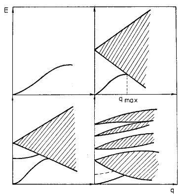
Figure 1: Schematic diagrams of excitation spectra in four microscopic models of theory of magnetism. Upper left: the Heisenberg model; upper right: the Hubbard model; lower left: the Zener model; lower right: the multiband Hubbard model.

In the Stoner band model the hydrodynamic pole is absent, there are no spin waves there. At the same time, the Stoner single-particle’s excitations are absent in the Heisenberg model’s spectrum. The Hubbard model [18, 19, 189] with narrow energy bands contains both types of excitations: the collective spin waves (the low energy spectrum) and Stoner single-particle’s excitations (the high-energy spectrum). This is a big advantage and flexibility of the Hubbard model in comparison to the Heisenberg model. The latter, nevertheless, is a very good approximation to the realistic behavior in the domain where the hydrodynamic description is applicable, that is, for long wavelengths and low energies. The quantum protectorate concept was applied to the quantum theory of magnetism by the author of this review in the paper [189], where a criterion of models of the quantum theory of magnetism applicability to description of concrete substances was formulated. The criterion is based on the analysis of the model’s low energy and high-energy spectra.

8 The Lawrence-Doniach Model

The Ginzburg-Landau model [310, 338] is a special form of the mean-field theory. This model operates with a pseudo-wave function $\Psi(\vec{r})$, which plays the role of a parameter of complex order, while the square of this function modulus $|\Psi(\vec{r})|^{2}$ should describe the local density of superconducting electrons. It is well known, that the Ginzburg-Landau theory is applicable if the temperature of the system is sufficiently close to its critical value $T_{c}$, and if the spatial variations of the functions $\Psi$ and of the vector potential $\vec{A}$ are not too large. The main assumption of the Ginzburg-Landau approach is the possibility to expand the free-energy density $f$ in a series under the condition, that the values of $\Psi$ are small, and its spatial variations are sufficiently slow. Then, we have

$$f=f_{n0}+\alpha|\Psi|^{2}+\frac{\beta}{2}|\Psi|^{4}+\frac{1}{2m^{*}}\Bigg{|}\bigg{(}-i\hbar\nabla+\frac{2e\vec{A}}{c}\bigg{)}\Psi\Bigg{|}^{2}+\frac{\hbar^{2}}{8\pi}.$$ (8.1)

The Ginzburg-Landau equations follow from an applications of the variational method to the proposed expansion of the free energy density in powers of $|\Psi|^{2}$ and $|\nabla\Psi|^{2},$ which leads to a pair of coupled differential equations for $\Psi(\vec{r})$ and the vector potential $\vec{A}$.
The Lawrence-Doniach model was formulated in the paper [339] for analysis of the role played by layered structures in superconducting materials [340, 341, 342]. The model considers a stack of parallel two dimensional superconducting layers separated by an insulated material (or vacuum), with a nonlinear interaction between the layers. It is also assumed that an external magnetic field is applied to the system. In some sense, the Lawrence-Doniach model can be considered as an anisotropic version of the Ginzburg- Landau model [310, 338]. More specifically, an anisotropic Ginzburg-Landau model can be considered as a continuous limit approximation to the Lawrence-Doniach model. However, when the coherence length in the direction perpendicular to the layers is less than the distance between the layers, these models are difficult to compare. In the framework of the approach used by Lawrence and Doniach the superconducting properties of the layered structure were considered under the assumption that in the superconducting state the free energy per cell relative to its value in the zero external field can be written in the following form

$$f(\vec{r})=\sum\limits_{i}^{n}\Bigg{[}\alpha_{i}(T)|\Psi_{i}(\vec{r})|^{2}+\beta|\Psi_{i}(\vec{r})|^{4}+\frac{1}{2m_{ab}}\Bigg{|}\bigg{(}-i\hbar\nabla+\frac{2e\vec{A}}{c}\bigg{)}\Psi_{i}(\vec{r})\Bigg{|}^{2}\Bigg{]}+$$

$$+\sum\limits_{<ij>}\eta_{ij}\Big{|}\Psi_{i}(\vec{r})-\Psi_{j}(\vec{r})\Big{|}^{2}.$$ (8.2)

Here, $\Psi_{i}(\vec{r})$ is the order parameter of the Ginzburg-Landau order of the layer number $i,$ ($\Psi_{i}(x,y)$ is a function of two variables), the operator $\nabla$ acts in the $x$-$y$ plane; $\vec{A}$ is the corresponding vector’s potential, $\alpha$ and $\beta$ are the usual Ginzburg-Landau parameters, $\eta_{ij}$ describes a positive Josephson interaction between the layers; and $<ij>$ denotes summation over neighboring layers. It is assumed that the layers correspond to planes $ab$, and the $c$ axis is perpendicular to these planes. Accordingly, the $z$ axis is aligned with $c$, and the coordinates $x$-$y$ belong to the plane $ab$. The quantities $\eta_{ij}$ are usually written as follows

$$\eta_{ij}=\frac{\hbar^{2}}{2m_{c}s^{2}}.$$ (8.3)

Here, $s$ is the distance between the layers. As one can see, for a rigorous treatment of the problem one has to take into account the anisotropy of the effective mass at the planes $ab$ and between them, $m_{ab}$ and $m_{c},$ respectively. Frequently, the distinction between these two types of anisotropy is ignored, and a quasi-isotropic case is considered. If we write down $\Psi_{i}$ in the form $\Psi_{i}=|\Psi_{i}|\exp(i\varphi_{i})$ and assume that all $|\Psi_{i}|$ are equal, then $\eta_{ij}$ is given by

$$\eta_{ij}=\frac{\hbar^{2}}{2m_{c}s^{2}}|\Psi_{i}|^{2}[1-\cos(\varphi_{i}-\varphi_{i-1})].$$ (8.4)

The coefficient $\alpha_{i}(T)$ for the layer number $i$ is given by

$$\alpha_{i}(T)=\alpha_{i}^{\prime}\frac{(T-T^{0}_{i})}{T^{0}_{i}},$$ (8.5)

where $T^{0}_{i}$ denotes the critical temperature for the layer number $i$. Next, one can consider the situation where $\Psi_{i}(\vec{r})=\Psi_{i}(r)$ and $\vec{A}=0.$ In the vicinity of $T_{c}$ the contribution from $\beta|\Psi_{i}|^{4}$ is small. Taking into account all these simplifications one can write down the free energy’s density in the following form

$$f=\sum\limits_{i}^{n}\alpha_{i}(T)|\Psi_{i}|^{2}+\sum\limits_{<ij>}\eta_{ij}|\Psi_{i}-\Psi_{j}|^{2}.$$ (8.6)

This is the quasi-isotropic approximation with single mass parameter $\alpha$. The Ginzburg-Landau equations follow from the free-energy extremum conditions with respect to variations of $\Psi_{i}$

$$\frac{\delta{}f}{\delta\Psi_{i}^{\ast}}=(\alpha_{i}+\eta_{i-1\;i}+\eta_{i\;i-1})\Psi_{i}-(\eta_{i-1\;i}\Psi_{i-1}+\eta_{i\;i+1}\Psi_{i+1})=0.$$ (8.7)

The corresponding secular equation is given by

$$\Big{|}(\alpha_{i}(T)+\eta_{i-1\;i}+\eta_{i\;i+1})\delta_{ij}-\eta_{ij}\delta_{i\;j\pm 1}\Big{|}=0.$$ (8.8)

It is assumed in the framework of the Lawrence-Doniach model [339] that the transition temperature corresponds to the largest root of the secular equation. In other words, one has to investigate solutions of the equation

$$\left|(T-T^{0}_{i}+\frac{\eta_{i-1\;i}}{\alpha_{i}^{\prime}}T^{0}_{i}+\frac{\eta_{i\;i+1}}{\alpha_{i}^{\prime}}T^{0}_{i})\delta_{ij}-\frac{\eta_{ij}}{\alpha_{i}^{\prime}}T^{0}_{i}\delta_{i\;j\pm 1}\right|=0,$$ (8.9)

or, in other form

$$\textrm{det}(TI-M)=0,\quad\textrm{where}\quad M_{ij}=\left(T^{0}_{i}-\frac{\eta_{i-1\;i}}{\alpha_{i}^{\prime}}T^{0}_{i}-\frac{\eta_{i\;i+1}}{\alpha_{i}^{\prime}}T^{0}_{i}\right)\delta_{ij}+\frac{\eta_{ij}}{\alpha_{i}^{\prime}}T^{0}_{i}\delta_{i\;j\pm 1}.$$ (8.10)

Thus, the problem is reduced to finding the maximal eigenvalue of the matrix $M$. If we take into account the external field, then the complete form of the Lawrence-Doniach equation [339] is given by

$$\alpha\Psi_{i}+\beta|\Psi_{i}|^{2}\Psi_{i}-\frac{\hbar^{2}}{2m_{ab}}\bigg{(}\nabla+i\frac{2e}{\hbar c}\vec{A}\bigg{)}^{2}\Psi_{i}$$

$$-\,\frac{\hbar^{2}}{2m_{c}s^{2}}\bigg{(}\Psi_{i+1}e^{2ieA_{z}s/\hbar c}-2\Psi_{i}-\Psi_{i-1}e^{2ieA_{z}s/\hbar c}\bigg{)}=0.$$ (8.11)

A large number of papers are devoted to investigations of the Lawrence-Doniach model and to development of various methods for its solution [340, 341, 342, 343, 344, 345]. In many respects this model corresponds to layered structures of high-temperature superconductors [346], and in particular to mercurocuprates [340, 341, 342]. A relativistic version of the Lawrence-Doniach model was studied in the paper [313], where violation of the local $U(1)$ gauge’s symmetry was considered by analogy with Higgs mechanism [303]. A spontaneous breaking of the global U(1) invariance is taking place through the superconducting condensate. The paper [313] also studied in detail the consequences of spontaneous symmetry breaking in connection with the Anderson-Higgs phenomenon [303]. As was mentioned already, the concept of spontaneous symmetry breaking corresponds to situations with symmetric action, but asymmetric realization (the vacuum condensate) in the low-energy regime. As a result the realization has a lower symmetry than the causing action [302, 308].
In essence, the Higgs mechanism [303] follows from the Anderson idea [302] on the connection between the gauge’s invariance breaking and appearance of the zero-mass collective mode in superconductors. Difference-differential equations for the order parameter, as well as for the vector potential at the plane and between the planes were also derived in the paper [313]. These equations correspond to the Klein-Gordon, Proca and sine-Gordon equations. The paper also contains a comparison of the superconducting phase shift $(\varphi_{i}-\varphi_{i-1})$ between the layers in the London limit with the standard sine-Gordon equation. A possible application of this approach to description of the high-temperature superconductivity in layered cuprates with a single plane in the elementary cell and with a weak Josephson interaction between the layers was also considered.
Thus, a systematic scheme for a phenomenological description of the macroscopic behavior of layered superconductors can be constructed by applying the covariance and gauge invariance principles to a four-dimensional generalization of the Lawrence-Doniach model. The Higgs mechanism [303] plays the role of a guiding idea, which allows one to place this approach on a deep and nontrivial foundation. The surprising formal simplicity of the Lawrence-Doniach model once again stresses the R. Peierls idea [93] on the efficiency of physical model creating.

9 Nonequilibrium Statistical Operators and Quasiaverages in the Theory of Irreversible Processes

It has been mentioned above that Bogoliubov’s quasiaverages concept [327, 328] plays an important role in equilibrium statistical mechanics. According to that concept, infinitely small perturbations can trigger macroscopic responses in the system if they break some symmetry and remove the related degeneracy (or quasidegeneracy) of the equilibrium state. As a result, they can produce macroscopic effects even when the perturbation magnitude is tend to zero, provided that happens after passing to the thermodynamic limit. D.N. Zubarev showed [347, 348] that the concepts of symmetry breaking perturbations and quasiaverages play an important role in the theory of irreversible processes as well [38]. The method of the construction of a nonequilibrium statistical operator [38] becomes especially deep and transparent when it is applied in the framework of the quasiaverage concept. The main idea of the papers [347, 348] was to consider infinitesimally small sources breaking the time-reversal symmetry of the Liouville equation

$$\frac{\partial\rho(t,0)}{\partial t}+\frac{1}{i\hbar}[\rho(t,0),H]=0$$ (9.1)

which become vanishingly small after a thermodynamic limiting transition.
The main idea of the method of a nonequilibrium statistical operator (NESO) [38] can be summarized as follows. In the scale of sufficiently large times the nonequilibrium state of the system can be described by some set of parameters $F_{m}(t)$, and one can find such a particular solution of the Liouville equation (9.1) which depends on time only through $F_{m}(t)$. The first argument of the operator $\rho(t,0)$ refers to an implicit time dependence. It is assumed that the nonequilibrium statistical ensemble can be characterized by a small set of relevant operators $P_{m}(t)$ (quasi-integrals of motion). The corresponding NESO is a functional of $P_{m}(t)$:

$$\rho(t)=\rho\{\ldots P_{m}(t)\ldots\}.$$ (9.2)

One can show, see [38], that if the statistical operator $\rho(t,0)$ satisfies the Liouville equation, then it is given by

$$\rho=\exp\bigl{(}\Lambda-\int^{0}_{-\infty}dt_{1}\sum_{m}G_{m}(t_{1})P_{m}(t_{1})\bigr{)};\quad\Lambda=1-\lambda,$$ (9.3)

where

$$G_{m}(t_{1})=\varepsilon e^{\varepsilon t_{1}}F_{m}(t+t_{1}),$$ (9.4)

$$\Lambda=\varepsilon\int^{0}_{-\infty}dt_{1}e^{\varepsilon t_{1}}\lambda(t+t_{1})=\lambda(t)-\int^{0}_{-\infty}dt_{1}e^{\varepsilon t_{1}}\dot{\lambda}(t+t_{1}).$$ (9.5)

Alternatively, it can be written as follows

$$\rho=\exp(\overline{\ln\rho_{q}})=\exp\bigl{(}\varepsilon\int^{0}_{-\infty}dt_{1}e^{\varepsilon t_{1}}e^{(}\frac{iHt_{1}}{\hbar})\ln\rho_{q}(t+t_{1})e^{(}\frac{-iHt_{1}}{\hbar})\bigr{)}=$$ (9.6)

$$\exp(-\overline{S(t,0)})=\exp(-\varepsilon\int^{0}_{-\infty}dt_{1}e^{\varepsilon t_{1}}S(t+t_{1},t_{1}))=$$

$$\exp\bigl{(}-S(t,0)+\int^{0}_{-\infty}dt_{1}e^{\varepsilon t_{1}}\dot{S}(t+t_{1},t_{1})\bigr{)},$$

where

$$\rho_{q}=\exp\left(\Omega-\sum_{m}F_{m}(t)P_{m}\right)\equiv\exp(-S(t,0)),\quad\Omega=\ln\textrm{Tr}\exp\left(-\sum_{m}F_{m}(t)P_{m}\right),$$ (9.7)

$$\dot{S}(t,0)=\frac{\partial S(t,0)}{\partial t}+\frac{1}{i\hbar}[S(t,0),H];$$ (9.8)

$$\dot{S}(t,t_{1})=\exp\left(\frac{iHt_{1}}{\hbar}\right)\dot{S}(t,0)\exp\left(\frac{-iHt_{1}}{\hbar}\right).$$

Here, $\rho_{q}$ is the quasi-equilibrium statistical operator, which corresponds to the extremum value of the information’s entropy

$$S=-\textrm{Tr}(\rho\ln\rho),$$ (9.9)

under the additional conditions that $\textrm{Tr}(\rho P_{m})=\langle P_{m}\rangle_{q};\quad\textrm{Tr}\rho=1.$ In this case

$$\frac{\delta\Phi}{\delta F_{m}}=-\langle P_{m}\rangle_{q};\quad\langle\ldots\rangle_{q}=\textrm{Tr}(\rho_{q}\ldots),$$ (9.10)

$$\Phi(\rho)=-\textrm{Tr}(\rho\ln\rho)-\sum_{m}F_{m}\textrm{Tr}(\rho P_{m})+\lambda\textrm{Tr}\rho,$$ (9.11)

$$\langle P_{m}\rangle^{t}=\langle P_{m}\rangle^{t}_{q}.$$ (9.12)

The quantum Liouville equation (9.1) (as well as the classical one) is invariant with respect to the time reversal. One can show [347, 348] that $\rho(t,0)$ satisfies the Liouville equation with an additional infinitesimally small (proportional to $\varepsilon$) source-term in the right hand side, and we send $\varepsilon$ to zero after the thermodynamic limit. Indeed, let us consider the equation

$$\frac{\partial\rho_{\varepsilon}}{\partial t}+\frac{1}{i\hbar}[\rho_{\varepsilon},H]=-\varepsilon(\rho_{\varepsilon}-\rho_{q})$$ (9.13)

or, equivalently,

$$\frac{\partial\ln\rho_{\varepsilon}}{\partial t}+\frac{1}{i\hbar}[\ln\rho_{\varepsilon},H]=-\varepsilon(\ln\rho_{\varepsilon}-\ln\rho_{q}),$$ (9.14)

where $\varepsilon\rightarrow 0$ after passage to the thermodynamic limit. Equation (9.13) is an analogue of the corresponding equation in the quantum scattering theory [349, 350]. The introduction of infinitely small sources in the Liouville equation corresponds to imposing the following boundary conditions

$$\exp\left(\frac{iHt_{1}}{\hbar}\right)\left(\rho(t+t_{1})-\rho_{q}(t+t_{1})\right)\exp\left(\frac{-iHt_{1}}{\hbar}\right)\rightarrow 0.$$ (9.15)

Here,$t_{1}\rightarrow-\infty$ after the thermodynamic limit. It was shown in the papers [38, 347, 348] that the operator$\rho_{\varepsilon}$ is given by

$$\rho_{\varepsilon}(t,t)=\varepsilon\int^{t}_{-\infty}dt_{1}e^{\varepsilon(t_{1}-t)}\rho_{q}(t_{1},t_{1})=\varepsilon\int^{0}_{-\infty}dt_{1}e^{\varepsilon t_{1}}\rho_{q}(t+t_{1},t+t_{1}).$$ (9.16)

Here, the first argument in $\rho(t,t)$ refers to the implicit time dependence via the parameters $F_{m}(t)$, while the second argument refers to the time dependence via the Heisenberg representation. The desired statistical operator is given by

$$\rho_{\varepsilon}=\rho_{\varepsilon}(t,0)=\overline{\rho_{q}(t,0)}=\varepsilon\int^{0}_{-\infty}dt_{1}e^{\varepsilon t_{1}}\rho_{q}(t+t_{1},t_{1}).$$ (9.17)

Hence, the nonequilibrium statistical operator is given by

$$\rho=Q^{-1}\exp\left(-\sum_{m}B_{m}\right)=Q^{-1}\exp\left(-\sum_{m}\varepsilon\int^{0}_{-\infty}dt_{1}e^{\varepsilon t_{1}}\left(F_{m}(t+t_{1})P_{m}(t_{1})\right)\right)=$$ (9.18)

$$Q^{-1}\exp\left(-\sum_{m}F_{m}(t)P_{m}+\sum_{m}\int^{0}_{-\infty}dt_{1}e^{\varepsilon t_{1}}[\dot{F}_{m}(t+t_{1})P_{m}(t_{1})+F_{m}(t+t_{1})\dot{P}_{m}(t_{1})]\right).$$

One can rewrite Eq. (9.14) in the following form

$$\frac{d}{dt}\left(e^{\varepsilon t}\ln\rho(t,t)\right)=\varepsilon e^{\varepsilon t}\ln\rho_{q}(t,t),$$ (9.19)

where

$$\ln\rho(t,t)=U^{\dagger}(t,0)\ln\rho(t,0)U(t,0);\quad U(t,0)=\exp\left(\frac{iHt}{\hbar}\right).$$ (9.20)

Integrating Eq. (9.19) over the interval $(-\infty,0)$ we obtain

$$\ln\rho(t,t)=\varepsilon\int^{0}_{-\infty}dt_{1}e^{\varepsilon t_{1}}\ln\rho_{q}(t+t_{1},t+t_{1}).$$ (9.21)

It is assumed that $\lim_{\varepsilon\rightarrow 0^{+}}\ln\rho(t,t)=0$. Therefore,

$$\rho(t,0)=\exp\left(-\varepsilon\int^{0}_{-\infty}dt_{1}e^{\varepsilon t_{1}}\ln\rho_{q}(t+t_{1},t_{1})\right)=\exp\overline{\left(\ln\rho_{q}(t,0)\right)}\equiv\exp\overline{\left(-S(t,0)\right)}.$$ (9.22)

The average value of any dynamic variable $A$ is now given by

$$\langle A\rangle=\lim_{\varepsilon\rightarrow 0^{+}}\textrm{Tr}(\rho(t,0)A).$$ (9.23)

We see that the above average is in fact nothing else but a quasiaverage. The normalization of the quasi-equilibrium distribution $\rho_{q}$ is preserved if

$$\textrm{Tr}(\rho(t,0)P_{m})=\langle P_{m}\rangle=\langle P_{m}\rangle_{q};\quad\textrm{Tr}\rho=1.$$ (9.24)

Thus, one can assert that the origin of the irreversibility effect is closely related to the violation of the time-reversal symmetry [351], as well as to the notion of quasiaverages from statistical mechanics [38, 347, 348].

9.1 Generalized Kinetic Equations

The NESO method [38] found wide applications in various problems of statistical mechanics. An important contribution to the development of the kinetic equations’ theory in the framework of NESO method was made by L.A. Pokrovskii [352, 353, 354]. Generalized kinetic and transport equations describing the time evolution of the variables $\langle P_{m}\rangle$ and $F_{m}(t)$ are obtained by averaging the equation of motion for $P_{m}$ over the derived NESO

$$\langle P_{m}\rangle=-\frac{\delta\Omega}{\delta F_{m}(t)};\quad F_{m}(t)=\frac{\delta S}{\delta\langle P_{m}\rangle}.$$ (9.25)

The generalized transport equations are given by

$$\langle\dot{P}_{m}\rangle=-\sum_{n}\frac{\delta^{2}\Omega}{\delta F_{m}(t)\delta F_{n}(t)}\dot{F}_{n}(t);\quad\dot{F}_{m}(t)=\sum_{n}\frac{\delta^{2}S}{\delta\langle P_{m}\rangle\delta\langle P_{n}\rangle}\langle\dot{P}_{n}\rangle.$$ (9.26)

The corresponding entropy production can be written down in the following form

$$\dot{S}(t)=\langle\dot{S}(t,0)\rangle=-\sum_{m}\langle\dot{P}_{m}\rangle F_{m}(t)=-\sum_{n,m}\frac{\delta^{2}\Omega}{\delta F_{m}(t)\delta F_{n}(t)}\dot{F}_{n}(t)F_{m}(t).$$ (9.27)

The two equations in (9.26) are mutually conjugate, and together with Eq. (9.27) they form a complete system of equations for calculation of the quantities $\langle P_{m}\rangle$ and $F_{m}$.
Now, following the paper [354], we are going to write down kinetic equations for a system with weak interaction. The corresponding Hamiltonian is given by

$$H=H_{0}+V.$$ (9.28)

Here, $H_{0}$ is the Hamiltonian of noninteracting particles (or quasiparticles) and $V$ is the interaction operator. As the set of relevant operators we choose the operators $P_{m}=P_{k}$ of the form $a^{\dagger}_{k}a_{k}$ or $a^{\dagger}_{k}a_{k+q}.$ Here, $a^{\dagger}_{k}$ and $a_{k}$ are the usual creation and the annihilation operators (either Fermi or Bose). We begin with the following equations of motion:

$$\dot{P}_{k}=\frac{1}{i\hbar}[P_{k},H].$$ (9.29)

It is usually assumed that

$$[P_{k},H_{0}]=\sum_{l}c_{kl}P_{l},$$ (9.30)

where $c_{kl}$ are some coefficients (c-numbers).
According to Eq. (9.18) we have

$$\rho=Q^{-1}\exp\left(-\sum_{k}F_{k}(t)P_{k}+\sum_{k}\int^{0}_{-\infty}dt_{1}e^{\varepsilon t_{1}}[\dot{F}_{k}(t+t_{1})P_{k}(t_{1})+F_{k}(t+t_{1})\dot{P}_{k}(t_{1})]\right).$$ (9.31)

Keeping in mind that $\langle P_{k}\rangle=\langle P_{k}\rangle_{q},$ we can write down the generalized kinetic equations [354] for $\langle P_{k}\rangle$ as follows

$$\frac{d\langle P_{k}\rangle}{dt}=\frac{1}{i\hbar}\langle[P_{k},H]\rangle=\frac{1}{i\hbar}\sum_{l}c_{kl}\langle P_{l}\rangle+\frac{1}{i\hbar}\langle[P_{k},V]\rangle.$$ (9.32)

The right hand side of Eq. (9.32) contains the generalized collision integral, which, using an expansion in powers of $V$, can be written as follows

$$\frac{d\langle P_{k}\rangle}{dt}=L^{0}_{k}+L^{1}_{k}+L^{21}_{k}+L^{22}_{k},$$ (9.33)

where

$$L^{0}_{k}=\frac{1}{i\hbar}\sum_{l}c_{kl}\langle P_{l}\rangle_{q},$$ (9.34)

$$L^{1}_{k}=\frac{1}{i\hbar}\langle[P_{k},V]\rangle_{q},$$ (9.35)

$$L^{21}_{k}=\frac{1}{\hbar^{2}}\int^{0}_{-\infty}dt_{1}e^{\varepsilon t_{1}}\langle[V(t_{1}),[P_{k},V]]\rangle_{q},$$ (9.36)

$$L^{22}_{k}=\frac{1}{\hbar^{2}}\int^{0}_{-\infty}dt_{1}e^{\varepsilon t_{1}}\langle[V(t_{1}),i\hbar\sum_{l}P_{l}\frac{\partial L^{1}_{k}(\ldots\langle P_{l}\rangle\ldots)}{\partial\langle P_{l}\rangle}]\rangle_{q}.$$ (9.37)

Analogously one can find the higher-order terms $V^{3}$, $V^{4}$ and so on.

9.2 Generalized Kinetic Equations for a System in a Thermal Bath

The papers [355, 356, 357] (see also [7]) generalize the equations in (9.32) for the case of a system interacting with a thermal bath. The concept of a thermal bath or heat reservoir is fairly complicated and has certain specific features [358]. According to the standard definition, a thermal bath is a system with, effectively, an infinite number of degrees of freedom. A thermal bath is a heat reservoir maintaining the investigated system under a particular temperature. Following Bogoliubov [359], we will assume that a thermal bath is a source of stochasticity for a small subsystem (which in an extreme situation can be just a single particle). Such a small subsystem can be, for example, an atomic or a molecular system interacting with an electromagnetic field, or a system of nuclear or electron spins interacting with the crystal lattice, etc. We will describe the entire system by the Hamiltonian

$$H=H_{1}+H_{2}+V,$$ (9.38)

where

$$H_{1}=\sum_{\alpha}E_{\alpha}a^{\dagger}_{\alpha}a_{\alpha};\quad V=\sum_{\alpha,\beta}\Phi_{\alpha\beta}a^{\dagger}_{\alpha}a_{\beta},\quad\Phi_{\alpha\beta}=\Phi^{\dagger}_{\beta\alpha}.$$ (9.39)

Here, $H_{1}$ is the Hamiltonian of the small subsystem; $a^{\dagger}_{\alpha}$, $a_{\alpha}$ are the creation and annihilation operators of quasiparticles with the energies $E_{\alpha}$ in the small subsystem; $V$ is the operator describing the interaction between the small subsystem and the thermal bath; and $H_{2}$ is the thermal bath’s Hamiltonian, which we do not write down explicitly. The quantities $\Phi_{\alpha\beta}$ are operators acting on the thermal bath’s degrees of freedom. We assume that the state of the system can be characterized by a set of operators $\langle P_{\alpha\beta}\rangle=\langle a^{\dagger}_{\alpha}a_{\beta}\rangle$, and the state of the thermal bath by the operator $\langle H_{2}\rangle$. Here, $\langle\ldots\rangle$ denotes the averaging with respect to the NESO, which is defined as follows:

$$\rho_{q}(t)=\exp(-S(t,0)),\quad S(t,0)=\Omega(t)+\sum_{\alpha\beta}P_{\alpha\beta}F_{\alpha\beta}(t)+\beta H_{2},$$ (9.40)

$$\Omega=\ln\textrm{Tr}\exp(-\sum_{\alpha\beta}P_{\alpha\beta}F_{\alpha\beta}(t)-\beta H_{2}).$$

Here, $F_{\alpha\beta}(t)$ are the thermodynamic parameters conjugate to $P_{\alpha\beta},$ $\beta$ is the inverse temperature of the thermal bath. All operators are considered in the Heisenberg representation. We write down the nonequilibrium statistical operator as follows

$$\rho(t)=\exp(-\overline{S(t,0)}),$$ (9.41)

$$\overline{S(t,0)}=\varepsilon\int^{0}_{-\infty}dt_{1}e^{\varepsilon t_{1}}\left(\Omega(t+t_{1})+\sum_{\alpha\beta}P_{\alpha\beta}F_{\alpha\beta}(t)+\beta H_{2}\right).$$

The parameters $F_{\alpha\beta}(t)$ are determined by the condition $\langle P_{\alpha\beta}\rangle=\langle P_{\alpha\beta}\rangle_{q}$. To derive the kinetic equations we will use an expansion over the small parameter in the interaction $V$. It is also assumed that the equation $\langle\Phi_{\alpha\beta}\rangle_{q}=0$. holds. It is convenient to rewrite $\rho_{q}$ as follows

$$\rho_{q}=\rho_{1}\rho_{2}=Q^{-1}_{q}\exp(-L_{0}(t)),$$ (9.42)

where

$$\rho_{1}=Q^{-1}_{1}\exp\left(-\sum_{\alpha\beta}P_{\alpha\beta}F_{\alpha\beta}(t)\right);\quad Q_{1}=\textrm{Tr}\exp\left(-\sum_{\alpha\beta}P_{\alpha\beta}F_{\alpha\beta}(t)\right),$$ (9.43)

$$\rho_{2}=Q^{-1}_{2}e^{-\beta H_{2}};\quad Q_{2}=\textrm{Tr}\exp(-\beta H_{2}),$$ (9.44)

$$Q_{q}=Q_{1}Q_{2};\quad L_{0}=\sum_{\alpha\beta}P_{\alpha\beta}F_{\alpha\beta}(t)+\beta H_{2}.$$ (9.45)

We begin from the following relationship:

$$\frac{d\langle P_{\alpha\beta}\rangle}{dt}=\frac{1}{i\hbar}\langle[P_{\alpha\beta},H]\rangle=\frac{1}{i\hbar}(E_{\beta}-E_{\alpha})\langle P_{\alpha\beta}\rangle+\frac{1}{i\hbar}\langle[P_{\alpha\beta},V]\rangle.$$ (9.46)

We terminate the expansions at the second order terms in $V$. The kinetic equations for the quantities $\langle P_{\alpha\beta}\rangle$ of a system in a thermal bath are given by

$$\frac{d\langle P_{\alpha\beta}\rangle}{dt}=\frac{1}{i\hbar}(E_{\beta}-E_{\alpha})\langle P_{\alpha\beta}\rangle-\frac{1}{\hbar^{2}}\int^{0}_{-\infty}dt_{1}e^{\varepsilon t_{1}}\langle\left[[P_{\alpha\beta},V],V(t_{1})\right]\rangle_{q}.$$ (9.47)

These equations generalize the results of the paper [354] for a system in a thermal bath. One can show that the choice of the concrete model’s form for the Hamiltonian (9.38) is not essential. For arbitrary $H_{1}$ and $V$, and for some set of variables $\langle P_{k}\rangle$ satisfying the condition $[H_{1},P_{k}]=\sum_{l}c_{kl}P_{l}$, one can construct a quasi-equilibrium statistical operator $\rho_{q}$ in the following form

$$\rho_{q}=Q^{-1}_{q}\exp\left(-\sum_{k}P_{k}F_{k}(t)-\beta H_{2}\right).$$ (9.48)

Here, $F_{k}(t)$ are the parameters conjugate to $\langle P_{k}\rangle$. The kinetic equations for $\langle P_{k}\rangle$ are given by

$$\frac{d\langle P_{k}\rangle}{dt}=\frac{i}{\hbar}\sum_{l}c_{kl}\langle P_{l}\rangle-\frac{1}{\hbar^{2}}\int^{0}_{-\infty}dt_{1}e^{\varepsilon t_{1}}\langle\left[[P_{k},V],V(t_{1})\right]\rangle_{q}.$$ (9.49)

9.3 A Schrödinger-Type Equation for a Dynamic System in a Thermal Bath

Following the papers [7, 355, 356, 357], we consider now the behavior of a small dynamical subsystem with a Hamiltonian $H_{1}$, which interacts with a thermal bath described by the Hamiltonian $H_{2}$. As the operators characterizing the state of the small subsystem we choose the operators $a^{\dagger}_{\alpha},a_{\alpha}$, and $n_{\alpha}=a^{\dagger}_{\alpha}a_{\alpha}$. In this case the quasi-equilibrium statistical operator $\rho_{q}$ is given by

$$\rho_{q}=\exp\left(\Omega-\sum_{\alpha}(f_{\alpha}(t)a_{\alpha}+f^{\dagger}_{\alpha}(t)a^{\dagger}_{\alpha}+F_{\alpha}(t)n_{\alpha})-\beta H_{2}\right)\equiv\exp(-S(t,0)),$$ (9.50)

$$\Omega=\ln\textrm{Tr}\exp\left(-\sum_{\alpha}(f_{\alpha}(t)a_{\alpha}+f^{\dagger}_{\alpha}(t)a^{\dagger}_{\alpha}+F_{\alpha}(t)n_{\alpha})-\beta H_{2}\right).$$

Here, $f_{\alpha},f^{\dagger}_{\alpha}$ and $F_{\alpha}$, play the role of Lagrange multipliers. They are the parameters conjugate to $\langle a_{\alpha}\rangle_{q},\langle a^{\dagger}_{\alpha}\rangle_{q}$ and $\langle n_{\alpha}\rangle_{q}$:

$$\langle a_{\alpha}\rangle_{q}=-\frac{\delta\Omega}{\delta f_{\alpha}(t)},\quad\langle n_{\alpha}\rangle_{q}=-\frac{\delta\Omega}{\delta F_{\alpha}(t)},\quad\frac{\delta S}{\delta\langle a_{\alpha}\rangle_{q}}=f_{\alpha}(t),\quad\frac{\delta S}{\delta\langle n_{\alpha}\rangle_{q}}=F_{\alpha}(t).$$ (9.51)

The quantities $a_{\alpha},\,a^{\dagger}_{\alpha}$ in the statistical operator can be interpreted as sources of quantum noise (those terms break the spin conservation law in the case of fermions; see the papers [7, 357]). Let us write down the quasi-equilibrium statistical operator as follows

$$\rho_{q}=\rho_{1}\rho_{2},$$ (9.52)

where

$$\rho_{1}=\exp\left(\Omega_{1}-\sum_{\alpha}(f_{\alpha}(t)a_{\alpha}+f^{\dagger}_{\alpha}(t)a^{\dagger}_{\alpha}+F_{\alpha}(t)n_{\alpha})\right)$$ (9.53)

$$\Omega_{1}=\ln\textrm{Tr}\exp\left(-\sum_{\alpha}(f_{\alpha}(t)a_{\alpha}+f^{\dagger}_{\alpha}(t)a^{\dagger}_{\alpha}+F_{\alpha}(t)n_{\alpha})\right)$$

$$\rho_{2}=\exp\left(\Omega_{2}-\beta H_{2}\right),\quad\Omega_{2}=\ln\textrm{Tr}\exp\left(-\beta H_{2}\right)$$ (9.54)

As a result we obtain the expression (9.41) for the NESO $\rho$. We assume that the following conditions are satisfied:

$$\langle a_{\alpha}\rangle_{q}=\langle a_{\alpha}\rangle,\quad\langle a^{\dagger}_{\alpha}\rangle_{q}=\langle a^{\dagger}_{\alpha}\rangle,\quad\langle n_{\alpha}\rangle_{q}=\langle n_{\alpha}\rangle.$$ (9.55)

We start from the equations of motion

$$i\hbar\frac{d\langle a_{\alpha}\rangle}{dt}=\langle[a_{\alpha},H_{1}]\rangle+\langle[a_{\alpha},V]\rangle,$$ (9.56)

$$i\hbar\frac{d\langle n_{\alpha}\rangle}{dt}=\langle[n_{\alpha},H_{1}]\rangle+\langle[n_{\alpha},V]\rangle.$$ (9.57)

In the second order in $V$ we obtain

$$i\hbar\frac{d\langle a_{\alpha}\rangle}{dt}=E_{\alpha}\langle a_{\alpha}\rangle+\frac{1}{i\hbar}\int^{0}_{-\infty}dt_{1}e^{\varepsilon t_{1}}\langle\left[[a_{\alpha},V],V(t_{1})\right]\rangle_{q},$$ (9.58)

$$i\hbar\frac{d\langle n_{\alpha}\rangle}{dt}=\frac{1}{i\hbar}\int^{0}_{-\infty}dt_{1}e^{\varepsilon t_{1}}\langle\left[[n_{\alpha},V],V(t_{1})\right]\rangle_{q}.$$ (9.59)

Here, $V(t_{1})$ denotes the operator $V$ in the interaction representation. The expansion yields

$$i\hbar\frac{d\langle a_{\alpha}\rangle}{dt}=E_{\alpha}\langle a_{\alpha}\rangle+$$

$$\frac{1}{i\hbar}\int^{0}_{-\infty}dt_{1}e^{\varepsilon t_{1}}\left(\sum_{\beta\mu\nu}\langle\Phi_{\alpha\beta}\phi_{\mu\nu}(t_{1})\rangle_{q}\langle a_{\beta}a^{\dagger}_{\mu}a_{\nu}\rangle_{q}-\langle\phi_{\mu\nu}(t_{1})\Phi_{\alpha\beta}\rangle_{q}\langle a^{\dagger}_{\mu}a_{\nu}a_{\beta}\rangle_{q}\right),$$ (9.60)

where $\phi_{\mu\nu}(t_{1})=\Phi_{\mu\nu}(t_{1})\exp(\frac{i}{\hbar}(E_{\mu}-E_{\nu})t_{1})$, or, equivalently

$$i\hbar\frac{d\langle a_{\alpha}\rangle}{dt}=E_{\alpha}\langle a_{\alpha}\rangle+\frac{1}{i\hbar}\sum_{\beta\mu}\int^{0}_{-\infty}dt_{1}e^{\varepsilon t_{1}}\langle\Phi_{\alpha\mu}\phi_{\mu\beta}(t_{1})\rangle_{q}\langle a_{\beta}\rangle+$$ (9.61)

$$\frac{1}{i\hbar}\sum_{\beta\mu\nu}\int^{0}_{-\infty}dt_{1}e^{\varepsilon t_{1}}\langle[\Phi_{\alpha\nu},\phi_{\mu\nu}(t_{1})]\rangle_{q}\langle a^{\dagger}_{\mu}a_{\nu}a_{\beta}\rangle_{q}.$$

Therefore, we obtain

$$i\hbar\frac{d\langle a_{\alpha}\rangle}{dt}=E_{\alpha}\langle a_{\alpha}\rangle+\frac{1}{i\hbar}\sum_{\beta\mu}\int^{0}_{-\infty}dt_{1}e^{\varepsilon t_{1}}\langle\Phi_{\alpha\mu}\phi_{\mu\beta}(t_{1})\rangle_{q}\langle a_{\beta}\rangle.$$ (9.62)

Using the spectral representations for the correlation functions we can write down

$$i\hbar\frac{d\langle a_{\alpha}\rangle}{dt}=E_{\alpha}\langle a_{\alpha}\rangle+\sum_{\beta}K_{\alpha\beta}\langle a_{\beta}\rangle,$$ (9.63)

where $K_{\alpha\beta}$ are defined as follows:

$$\frac{1}{i\hbar}\sum_{\mu}\int^{0}_{-\infty}dt_{1}e^{\varepsilon t_{1}}\langle\Phi_{\beta\mu}\phi_{\mu\nu}(t_{1})\rangle_{q}=$$ (9.64)

$$\frac{1}{2\pi}\sum_{\mu}\int^{+\infty}_{-\infty}d\omega\frac{J_{\mu\nu,\beta\mu}(\omega)}{\hbar\omega-E_{\mu}-E_{\nu}+i\varepsilon}=K_{\beta\nu}.$$

Thus, we have obtained a Schrödinger-type equation for the mean amplitudes $\langle a_{\alpha}\rangle$. In a certain sense this equation is an analogue (or a generalization) of the Schrödinger equation for the case of a particle moving in a medium. Let us consider this analogy in a more detail. First, we write down the analogue of the wave function in the following form

$$\psi(\vec{r})=\sum_{\alpha}\chi_{\alpha}(\vec{r})\langle a_{\alpha}\rangle.$$ (9.65)

Here, $\{\chi_{\alpha}(\vec{r})\}$ is a complete orthonormal set of single-particle eigenfunctions of the operator $\left(-\frac{\hbar^{2}}{2m}\nabla^{2}+v(\vec{r})\right)$, where $v(\vec{r})$ is the potential energy,

$$\left(-\frac{\hbar^{2}}{2m}\nabla^{2}+v(\vec{r})\right)\chi_{\alpha}(\vec{r})=E_{\alpha}\chi_{\alpha}(\vec{r}).$$ (9.66)

Thus, the quantity $\psi(\vec{r})$ plays the role of a wave function describing a particle moving in a medium. Equation (9.63) can be rewritten in the following form

$$i\hbar\frac{\partial\psi(\vec{r})}{\partial t}=\left(-\frac{\hbar^{2}}{2m}\nabla^{2}+v(\vec{r})\right)\psi(\vec{r})+\int K(\vec{r},\vec{r^{\prime}})\psi(\vec{r^{\prime}})d\vec{r^{\prime}}.$$ (9.67)

The kernel $K(\vec{r},\vec{r^{\prime}})$ of the integral equation (9.67) is given by

$$K(\vec{r},\vec{r^{\prime}})=\sum_{\alpha\beta}K_{\alpha\beta}\chi_{\alpha}(\vec{r})\chi^{{\dagger}}_{\beta}(\vec{r^{\prime}})=\frac{1}{i\hbar}\sum_{\alpha,\beta,\mu}\int^{0}_{-\infty}dt_{1}e^{\varepsilon t_{1}}\langle\Phi_{\alpha\mu}\phi_{\mu\beta}(t_{1})\rangle_{q}\chi_{\alpha}(\vec{r})\chi^{{\dagger}}_{\beta}(\vec{r^{\prime}}).$$ (9.68)

We see that Eq. (9.67) can indeed be classified as a Schrödinger-type equation for a dynamical system in a thermal bath. It is interesting to note that very similar equations of the Schrödinger-type with a nonlocal interaction were used in the collision theory [360] for description of particle scattering on a cluster of many scattering centers.
In order to make clear some special features of Eq. (9.67) let us consider the translation operator $\exp(i\vec{q}\vec{p}/\hbar)$, $\vec{q}=\vec{r^{\prime}}-\vec{r},$ where $\vec{p}=-i\hbar\nabla_{r},$ Then, Eq. (9.67) can be rewritten in the following form

$$i\hbar\frac{\partial\psi(\vec{r})}{\partial t}=\left(-\frac{\hbar^{2}}{2m}\nabla^{2}+v(\vec{r})\right)\psi(\vec{r})+\sum_{p}D(\vec{r},\vec{p})\psi(\vec{r}),$$ (9.69)

where

$$D(\vec{r},\vec{p})=\int d^{3}qK(\vec{r},\vec{r}+\vec{q})e^{\frac{i\vec{q}\vec{p}}{\hbar}}.$$ (9.70)

It is reasonable to assume that the wave function $\psi(\vec{r})$ does not change very rapidly over distances comparable to the characteristic correlation length of the kernel $K(\vec{r},\vec{r^{\prime}}).$ Then, using the series expansion for $\exp(i\vec{q}\vec{p}/\hbar)$ in Eq. (9.69) we obtain in the zeroth order

$$i\hbar\frac{\partial\psi(\vec{r})}{\partial t}=\left(-\frac{\hbar^{2}}{2m}\nabla^{2}+v(\vec{r})+\textrm{Re}\,U(\vec{r})\right)\psi(\vec{r})+i\textrm{Im}\,U(\vec{r})\psi(\vec{r}),$$ (9.71)

where

$$U(\vec{r})=\textrm{Re}\,U(\vec{r})+i\textrm{Im}\,U(\vec{r})=\int d^{3}qK(\vec{r},\vec{r}+\vec{q}).$$ (9.72)

Equation (9.71) has the exact functional form of a Schrödinger equation with a complex potential well known in the collision theory [360]. Note that the introduction of the quantity $\psi(\vec{r})$ does not mean that the state of the small dynamical subsystem becomes pure. The state remains mixed because it is described by a statistical operator. The dynamics of the system is described by a system of coupled evolution equations for the quantities $f_{\alpha},f^{\dagger}_{\alpha}$ and $F_{\alpha}$. Note, that there were many attempts to derive a Schrödinger-type equation for a particle in a medium [361, 362, 363]. Korringa [361] tried to obtain such an equation in the form of an evolution equation with a non-hermitian Hamiltonian. However, his equation (cf. Eq. (29) from [361])

$$i\frac{\partial W^{\prime}}{\partial t}=\left(H^{\prime}(t)+h^{\prime}(t))+\frac{i}{2\theta}\frac{dh^{\prime}}{dt}+\ldots\right)W^{\prime}(t),$$ (9.73)

where $W^{\prime}(t)$ is a statistical density matrix describing the original system, is rather a modified Bloch equation. An attempt to derive a Schroedinger-type equation for a Brownian particle interacting with a thermal environment was made in the paper [362]. The evolution equation obtained there is given by

$$i\hbar\frac{\partial\psi}{\partial t}=-\frac{\hbar^{2}}{2m}\nabla^{2}\psi+V\psi+V_{R}\psi+[\frac{\hbar f}{2im}\ln(\frac{\psi}{\psi^{*}})+W(t)]\psi(\vec{r},t),$$ (9.74)

where

$$W(t)=-(\frac{\hbar f}{2im})\int\psi^{*}\ln(\frac{\psi}{\psi^{*}})\psi dr.$$ (9.75)

Here, $f$ is the friction coefficient, $V_{R}$ is a random potential, and $V_{R}(\vec{r},t)=-\vec{r}\vec{F}_{R}(t),$ where $\vec{F}_{R}(t)$ is a random vector-function of time. Excluding the function $W(t)$ with the help of the transformation

$$\psi(\vec{r},t)=\exp[i\theta(t)]\phi(\vec{r},t),$$ (9.76)

where

$$\theta(t)=-\hbar^{-1}\exp(-\frac{tf}{m})\int_{0^{t}}^{t}\exp(\frac{sf}{m})W(s)ds,$$

one obtains the equation for $\phi(\vec{r},t)$ in the following form

$$i\hbar\frac{\partial\phi}{\partial t}=-\frac{\hbar^{2}}{2m}\nabla^{2}\phi(\vec{r},t)+V(\vec{r})\phi(\vec{r},t)+V_{R}(\vec{r},t)\phi(\vec{r},t)+$$ (9.77)

$$\frac{\hbar f}{2im}\phi(\vec{r},t)\ln[\frac{\phi(\vec{r},t)}{\phi^{*}(\vec{r},t)}].$$

It is clear that the dynamic behavior of a particle in a dissipative environment is most accurately described by a Schrödinger-type equation with damping, see Eq.(9.67) above. This is actually the reason for applications of this equation in numerous problems of physics, physical chemistry, biophysics, and other areas [364, 365, 366, 367, 368, 369, 370, 371, 372]. A more detailed discussion of various aspects of dissipative behavior and of stochastic process in complex systems is given in the reviews [7, 373, 374, 375, 376].

10 Conclusion

In the present paper we have shown the determining role played by correlation effects in systematic microscopic descriptions of magnetic, electrical, and superconducting properties of complex substances. We have stressed that the approximation of tight-binding electrons and the method of model Hamiltonians are very effective tools for description of these substances. In many cases the methods of quantum statistical mechanics, many of which were formulated and developed by N.N. Bogoliubov, allow one to develop efficient approaches for solution of complicated problems from microscopic theory of correlation effects, especially in the case of strong electron correlations. The method of two-time temperature Green’s functions allows one to efficiently investigate the quasiparticle dynamics generated by the main model Hamiltonians from the quantum solid state theory and the quantum theory of magnetism. The method of quasiaverages allows one to take a deeper look at the problems of spontaneous symmetry breaking, as well as at the problems of symmetry and dissymmetry in the physics of condensed matter. Further development of the theory describing many-particle effects and investigations of more realistic models will allow one to gain more precise ideas on the effective interactions in the systems, which determine various phenomena, the main features of electron states, and therefore, the physical properties of real substances. The methods developed by N.N. Bogoliubov are and will remain the important core of a theoretician’s toolbox, and of the ideological basis behind this development.

11 Acknowledgements

The author recollects with gratefulness discussions of this review topics with N.N. Bogoliubov (21.08.1909-13.02.1992) and D.N. Zubarev (30.11.1917-16.07.1992). He is also grateful to Professor N.N. Bogoliubov, Jr., for valuable discussions and bringing the reference [286] to his attention.

References

- [1] J. W. Gibbs, Elementary Principles in Statistical Mechanics Developed with Especial Reference to the Rational Foundations of Thermodynamics (Yale Uni. Press, New Heaven, 1902).
- [2] U. I. Frankfurt and A. M. Frenk, Josiah Willard Gibbs (Nauka, Moscow, 1964) [in Russian].
- [3] N. N. Bogoliubov, Collected Works, in 12 Vols. (Nauka, Moscow, 2005-2009) [in Russian].
- [4] N. N. Bogoliubov and N. N. Bogoliubov, Jr., Introduction to Quantum Statistical Mechanics, 2nd ed. (World Scientific, Singapore, 2009).
- [5] A. N. Bogoliubov, N. N. Bogoliubov. The Life. The Scientific Activity (JINR Publishing, Dubna, 1996) [in Russian].
- [6] N. N. Bogoliubov, Jr. and D. P. Sankovich, N. N. Bogoliubov and Statistical Mechanics, Usp. Mat. Nauk 49, 21 (1994) [Russ. Math. Surv. 49, 19 (1994)].
- [7] A. L. Kuzemsky, Theory of Transport Processes and the Method of the Nonequilibrium Statistical Operator, Int. J. Mod. Phys. B 21, 2821-2949 (2007) [e-Preprint:arXiv:cond-mat/0707.0753].
- [8] R. W. van Boeyen, N. Watanabe, J. P. Doering, J. H. Moore, M. A. Coplan. Practical Means for the Study of Electron Correlation in Atoms, Phys. Rev. Lett. 92 223202 (2004).
- [9] R. E. Hummel. Understanding Materials Science: History, Properties, Applications. (Springer, Berlin, 2005).
- [10] R. C. O’Handley. Modern Magnetic Materials: Principles and Applications ( Wiley-Interscience, New York, 1999).
- [11] D. Shi et al., eds. Nanostructured Magnetic Materials and Their Applications (Springer, Berlin, 2001).
- [12] A. Planes, L. Manosa and A. Saxena, eds. Magnetism and Structure in Functional Materials. (Springer, Berlin, 2006).
- [13] C. P. Poole, H. A. Farach, R. J. Creswick, R. Prozorov, Superconductivity, 2nd ed. (Academic Press, New York, 2007).
- [14] H. Fredriksson, U. Akerlind. Physics of Functional Materials. ( John Wiley and Sons, New York, 2008).
- [15] C. G. Stefanita. From Bulk to Nano: The Many Sides of Magnetism (Springer Series in Materials Science, Vol.117) (Springer, Berlin, 2008).
- [16] S. V. Tyablikov, Methods in the Quantum Theory of Magnetism (Plenum Press, New York, 1967).
- [17] D. Mattis, The Theory of Magnetism (Springer, Berlin, 1988).
- [18] A. L. Kuzemsky, Neutron Scattering and Magnetic Properties of Transition Metals and Alloys, Fiz. Elem. Chastits At. Yadra 12, 366-423 (1981) [Sov. J. Part. Nucl. 12, 146 (1981)]
- [19] A. L. Kuzemsky, Fundamental Principles of the Physics of Magnetism and the Problem of Itinerant and Localized Electronic States. Communication JINR E17-2000-32, Dubna (2000).
- [20] A. L. Kuzemsky, Irreducible Green Functions Method and Many-Particle Interacting Systems on a Lattice. Rivista del Nuovo Cimento 25, 1 (2002) [e-Preprint: arXiv:cond-mat/0208219].
- [21] A. L. Kuzemsky, Correlation Effects in High Temperature Superconductors and Heavy Fermion Compounds. in: Superconductivity and Strongly Correlated Electron Systems, Eds. C. Noce, A. Romano, G. Scarpetta (World Scientific, Singapore, 1994), Pp.346–376.
- [22] A. L. Kuzemsky, A Self-consistent Theory of the Electron Correlation in the Hubbard Model. Teor.Mat.Fiz. 36 208-223 (1978) [Theor.Math.Phys. 36 692 (1979)].
- [23] A. L. Kuzemsky, Irreducible Green’s Function Method in Condensed Matter Physics, Doklady AN SSSR 309 323-326 (1989) [Sov.Phys.Dokl. 34 974 (1989)].
- [24] A. L. Kuzemsky, Generalized Mean Fields and Quasiparticle Interactions in the Hubbard Model. Nuovo Cimento, B 109 829–854 (1994).
- [25] G. Czycholl, A. L. Kuzemsky, S. Wermbter, New Interpolative Treatment of the Single-Impurity Anderson Model. Europhysics Lett. 34 133-138 (1996).
- [26] A. L. Kuzemsky, Quasiparticle Many-Body Dynamics of the Anderson Model. Int. J. Mod. Phys. B 10, 1895-1912 (1996).
- [27] A. L. Kuzemsky, Role of Correlation and Exchange for Quasiparticle Spectra of Magnetic and Diluted Magnetic Semiconductors. Physica B 355, 318-340 (2005) [e-Preprint: arXiv:cond-mat/0403266].
- [28] Steven G. Louie, Marvin L. Cohen, eds. Conceptual Foundations of Materials: A Standard Model for Ground- and Excited-State Properties (Elsevier, Amsterdam, 2006).
- [29] J. D. Livingston. Driving Force: The Natural Magic of Magnets. (Harvard University Press, Cambridge, Mass., 1996).
- [30] V. Weisskopf, Knowledge and Wonder ( Doubleday and Co., New York, 1962).
- [31] W. O. Gilbert, On the Magnet and Magnetic Bodies, and on the Great Magnet the Earth, Translated 1893 from Latin to English by Paul Fleury Mottelay, Dover Books.
- [32] N. G. Bochkarev, Magnetic Fields in Space (Nauka, Moscow, 1985) [in Russian].
- [33] W. H. Campbell, Earth Magnetism (Academic Press, New York, 2001).
- [34] M. T. Zuber, Model for Magnetic Mystery. Nature 421, 119 (2003).
- [35] S. V. Vonsovskii, Magnetism (Nauka, Moscow, 1971; Wiley, New York, 1971).
- [36] P. Weiss, L’hypothese du champ moleculaire et la propriete ferromagnetique. Journal de Physique. Theorique et Applique. Ser. 4, 6, 661 (1907) [in French].
- [37] J. S. Smart, Effective Field Theories of Magnetism (Saunders, London, 1966).
- [38] D. N. Zubarev, Nonequilibrium Statistical Thermodynamics (Consultant Bureau, New York, 1974).
- [39] M. Toda, R. Kubo, N. Saito. Statistical Physics: vol.1, Equilibrium Statistical Mechanics. (Berlin: Springer, 1992).
- [40] R. Kubo, M. Toda, N. Hashitsume. Statistical Physics: vol.2, Nonequilibrium Statistical Mechanics. (Berlin: Springer, 1991).
- [41] R. A. Minlos, Introduction to Mathematical Statistical Physics ( Amer. Math. Soc., Providence, RI, 2000).
- [42] P. J. Grout and N. H. March, Internal Energy versus Moment for Ferromagnets and Pyroelectrics. Phys.Rev. B 14, 4027 (1976).
- [43] N. H. March, A. M. L. Nip, and J. A. Tuszynski, Free Energy in Relation to Order Parameter in Magnets and Pyroelectrics. Intern. J. Quant. Chem. 30, 1549 (1996).
- [44] A. Misra, A. Ayuela, D. J. Klein, and N. H. March, Magnetically Ordered Materials: Relation Between Internal Energy, Magnetization and Applied Field. Phys. Lett. A 329, 396 (2004).
- [45] A. Ayuela and N. H. March, Spontaneous Magnetization Related to Internal Energy in an Assembly with Long-Range Interaction: Predicted Universal Features Fingerprints in Experimental Data from and . Phys. Lett. A 372, 5617 (2008).
- [46] C. Domb, The Critical Point (Taylor and Francis, London, 1996).
- [47] P. Weiss and G. Foex, Le Magnetisme (Colin, Paris, 1926) [in French].
- [48] Z. Wlodarski and J. Wlodarska, Analytical Approximation of the Dependence of Magnetic Material Properties on Temperature. The Intern. J. for Computation and Mathematics in Electrical and Electronic Engineering 17, 408 (1998).
- [49] M. D. Kuzmin and A. M. Tishin, Temperature Dependence of the Spontaneous Magnetization of Ferromagnetic Insulators: Does it obey the law? Phys. Lett. A 341, 240 (2005).
- [50] Z. Wlodarski, Analytical Description of Magnetization Curves. Physica B 373, 323 (2006).
- [51] Ya. G. Dorfman, Magnetic Properties and Structure of the Matter (GITTL, Moscow, 1955) [in Russian].
- [52] W. Weber, S. Riesen, and H. C. Siegmann, Magnetization Precession by Hot Spin Injection. Science 291, 1015 (2001).
- [53] C. Albert, L. Ferrari, J. Froehlich, and B. Schlein, Magnetism and the Weiss Exchange Field - A Theoretical Analysis Motivated by Recent Experiments. J. Stat. Phys. 125, 77 (2006).
- [54] L. Neel, Magnetism and Local Molecular Fields. Usp. Fiz. Nauk 107, 185 (1972).
- [55] R. M. White, Quantum Theory of Magnetism, 3rd ed. (Springer, Berlin, 2007).
- [56] J. Stohr and H. C. Siegmann, Magnetism. From Fundamentals to Nanoscale Dynamics (Springer, Berlin, 2006).
- [57] B. A. Vvedenskii and G. S. Landsberg, Contemporary Study of Magnetism (OGIZ, Moscow, 1929) [in Russian].
- [58] E. C. Stoner, Magnetism and Atomic Structure (Dutton, New York, 1926).
- [59] J. H. van Vleck, The Theory of Electric and Magnetic Susceptibilities (Clarendon, Oxford, 1932).
- [60] F. Bloch, Molecular Theory of Magnetism (ONTI, Kiev, 1934) [in Russian].
- [61] K. Yosida, Theory of Magnetism (Springer, Berlin, 1996).
- [62] C. Herring, Exchange Interactions among Itinerant Electrons (Academic, New York, 1966).
- [63] H. J. Zeiger and G. W. Pratt, Magnetic Interactions in Solids (Clarendon, Oxford, 1973).
- [64] B. Barbara, D. Gignoux, and C. Vettier, Lectures on Modern Magnetism (Springer, Berlin, 1988).
- [65] W. J. Caspers, Spin Systems (World Scientific, Singapore, 1989).
- [66] A. Aharoni, Introduction to the Theory of Ferromagnetism (Clarendon, Oxford, 1996).
- [67] S. Chikazumi, Physics of Ferromagnetism, 2nd ed. (Clarendon, Oxford, 1997).
- [68] K. W. H. Stevens, Magnetic Ions in Crystals (Princeton Univ., Princeton, 1997).
- [69] L. J. de Jongh and A. R. Miedema, Experiments on Simple Magnetic Model Systems. Adv. Phys. 50, 947 (2001).
- [70] Magnetism. I. Fundamentals. Eds. E. du Tremolet de Lacheisserir, D. Gignoux, M. Schlenker. (Springer, Berlin, 2002).
- [71] Magnetism. II. Materials and Applications. Eds. E. du Tremolet de Lacheisserir, D. Gignoux, M. Schlenker. (Springer, Berlin, 2005).
- [72] K. H. J. Buschow and F. R. De Boer, Physics of Magnetism and Magnetic Materials (Kluwer, New York, Boston, 2003).
- [73] N. Spaldin, Magnetic Materials: Fundamentals and Device Applications (Cambridge Univ., Cambridge, 2003).
- [74] Magnetic Heterostructures. Advances and Perspectives in Spinstructures and Spintransport, Ed. by H. Zabel, S. D. Bader (Springer, Berlin, 2007).
- [75] Modern Techniques for Characterizing Magnetic Materials, Ed. by Yimei Zhu (Kluwer, New York, Boston, 2005).
- [76] W. Marshall and S. Lovesey, Theory of Thermal Neutron Scattering (Clarendon, Oxford, 1971).
- [77] Neutron Scattering from Magnetic Materials, Ed. by Tapan Chatterji (Elsevier, Amsterdam, 2006).
- [78] Magneto-Optics, Ed. by S. Sugano, N. Kojima. (Springer, Berlin, 2000).
- [79] G. H. Lander, Studies of Magnetism with Synchrotron X-rays. Journal of Alloys and Compounds 250, 544 (1997).
- [80] Magnetism and Synchrotron Radiation, Eds. E. Beaurepaire et al. (Springer, Berlin, 2001).
- [81] Magnetism: A Synchrotron Radiation Approach, Eds. E. Beaurepaire et al. (Springer, Berlin, 2006).
- [82] G. V. Fetisov, Synchrotron Radiation. Methods for Structural Studies of Substances (Fizmatlit, Moscow, 2007) [in Russian].
- [83] Fifty Years of Neutron Diffraction, Ed. by G. E. Bacon (Adam Hilger, Bristol, 1986).
- [84] K. Yosida, Development of Magnetism Studies. in: Perspectives in Quantum Physics (Naukova Dumka, Kiev, 1982), p. 101 [in Russian].
- [85] J. van Vleck, Quantum Mechanics: The Key to Understanding Magnetism. Usp. Fiz. Nauk 127, 3 (1979).
- [86] S. Yamanaka et al., Chemical Bonding, Less Screening, and Hund’s Rule Revisited. Intern. J. Quant. Chem. 105, 687 (2005).
- [87] A. Mielke, Ferromagnetism in the Hubbard Model and Hund’s Rule. Phys. Lett. A 174, 443 (1993).
- [88] J. Froehlich and D. Ueltschi, Hund’s Rule and Metallic Ferromagnetism. J. Stat. Phys. 118, 973 (2005).
- [89] M. Massimi, Pauli’s Exclusion Principle: The Origin and Validation of a Scientific Principle (Cambridge Univ., Cambridge, 2005).
- [90] J. Callaway, Energy Band Theory (Academic Press, New York, 1964).
- [91] W. A. Harrison, Elementary Electronic Structure (World Scientific, Singapore, 1999).
- [92] R. M. Martin, Electronic Structure: Basic Theory and Practical Methods (Cambridge Univ., Cambridge, 2004).
- [93] R. Peierls, Model-Making in Physics, Contemp.Phys. 21, 3 (1980).
- [94] S. G. Brush, History of the Lenz-Ising Model. Rev. Mod. Phys. 39, 883 (1967).
- [95] S. Kobe, Ernst Ising - Physicist and Teacher. J. Stat. Phys. 88, 991 (1997).
- [96] The Collected Works of Lars Onsager, Eds. P. C. Hemmer et al. (World Scientific, Singapore, 1996).
- [97] G. Bennetin, G. Gallavotti, G. Jona-Lasinio, and A. L. Stella, On the Onsager-Yang-Value of the Spontaneous Magnetization. Commun. Math. Phys. 30, 45 (1973).
- [98] W. Heisenberg, Zur Theorie des Ferromagnetismus. Zeits. f. Physik 49, 619 (1928) [in German].
- [99] P. Dirac, Quantum Mechanics of Many-Electron Systems. Proc. Roy. Soc. A 123, 714 (1929).
- [100] J. H. Van Vleck, Nonorthogonality and Ferromagnetism. Phys. Rev. 49, 232 (1936).
- [101] C. Kittel, Ferromagnetism. Suppl. del Nuovo Cimento 6, 897 (1957).
- [102] J. H. Van Vleck, Models of Exchange Coupling in Ferromagnetic Media. Rev. Mod. Phys. 25, 220 (1953).
- [103] T. Arai, Exchange Interaction and Heisenberg’s Spin Hamiltonian. Phys. Rev. 126, 471 (1962).
- [104] C. Herring, On the Possibility of Saturated Ferromagnetism. Phys. Rev. B 11, 2056 (1975).
- [105] C. Carson, The Peculiar Notion of Exchange Forces - I. Origins in Quantum Mechanics 1926-1928. Studies in History and Philosophy of Modern Physics 27, 23 (1996).
- [106] J. H. Van Vleck, On the Theory of Antiferromagnetism. J. Chem. Phys. 9, 85 (1941).
- [107] C. J. Gorter, Antiferromagnetism. Suppl. del Nuovo Cimento. 6, 923 (1957).
- [108] W. J. O’Sullivan, W. A. Robinson, and W. W. Simmons, Sublattice Switching in Antiferromagnets. Phys. Rev. 124, 1317 (1961).
- [109] Antiferromagnetism and Ferrites, Ed. by Ya. G. Dorfman (Akad. Nauk SSSR, Moscow, 1962) [in Russian].
- [110] K. P. Belov et al., Rare-Earth Ferro- and Antiferromagnetics (Nauka, Moscow, 1965) [in Russian].
- [111] G. A. Smolenskii et al., Physics of Magnetic Dielectrics, Ed. by G. A. Smolenskii (Nauka, Leningrad, 1974) [in Russian]
- [112] G. A. Smolenskii and V. V. Lemanov, Ferrites and their Technical Applications (Nauka, Leningrad, 1975) [in Russian].
- [113] A. K. Zvezdin et al., Rare-Earth Ions in Magnetically Ordered Crystals (Nauka, Moscow, 1985) [in Russian].
- [114] S. A. Nikitin, Magnetic Properties of Rare Earth Metals and Their Alloys (Moscow State Univ., Moscow, 1989) [in Russian].
- [115] E. A. Turov et al., Symmetry and Physical Properties of Antiferromagnets (Fizmatlit, Moscow, 2001) [in Russian].
- [116] E. S. Borovik, V. V. Eremenko, and A. S. Mil’ner, Lectures on Magnetism (Fizmatlit, Moscow, 2005) [in Russian].
- [117] L. Neel, Proprietes Magnetiques des Ferrites. Ferrimagnetisme et Antiferromagnetisme (Magnetic Properties of Ferrites. Ferromagnetism and Antiferromagnetism), Annals de Physique 3, 137 (1948) [in French].
- [118] W. P. Wolf, Ferrimagnetism. Rep. Progr. Phys. 24, 212 (1961).
- [119] P. Quedec, Itineraire de Louis Neel des Aimants aux Grenats Ferrimagnetiques. Annals of Science 47, 261 (1990) [in French].
- [120] Selected Works of Louis Neel, Ed. by N. Kurti (Routledge, London, 1988).
- [121] Louis Neel, Un Siecle de Physique. (Odile Jacob, Paris, 1991) [in French].
- [122] M. Prevot and D. Dunlop, Louis Neel: 40 years of magnetism. Physics of the Earth and Planetary Interiors 126, Issues 1-2, 3 (2001).
- [123] P. W. Anderson, Ordering and Antiferromagnetism in Ferrites. Phys. Rev. 102, 1008 (1956).
- [124] A. H. Morrish, Canted Antiferromagnetism: Hematite (World Scientific, Singapore, 1994).
- [125] L. Neel, Annals de Physique 4, 249 (1949).
- [126] A. Aharoni, E. H. Frei, and M. Schierer, Curie Point and Origin of Weak Ferromagnetism in Hematite. Phys. Rev. 127, 439 (1962).
- [127] T. Moriya, New Mechanism of Anisotropic Superexchange Interaction. Phys. Rev. Lett. 4, 228 (1960).
- [128] T. Moriya, Anisotropic Superexchange Interaction and Weak Ferromagnetism. Phys. Rev. 117, 635 (1960).
- [129] S. T. Lin, Magnetic Properties of Hematite Single Crystals.I. Magnetization Isotherms, Antiferromagnetic Susceptibility, and Weak Ferromagnetism of a Natural Crystal. Phys. Rev. 116, 1447 (1959).
- [130] P. J. Flanders and J. P. Remeika, The Magnetic Properties of Hematite Single Crystals. Phil. Mag. 11, 1271 (1965). 1
- [131] D. J. Dunlop, Hematite: Intrinsic and Defect Ferromagnetism. Science 169, 858 (1970).
- [132] A. L. Kuzemsky and E. A. Tkachenko, Scattering of Slow Neutrons on Hematite in Strong Magnetic Fields, Fiz. Tverd. Tela 16, 3082-3088 (1974) [Sov. Phys. Solid State 16, 1989 (1974)].
- [133] L. Suber et al., Structural and Magnetic Properties of Nanoparticles. Appl. Organometallic Chemistry 12, 347 (1998).
- [134] F. Bodker and S. Morup, Size Dependence of the Properties of Hematite Nanoparticles. Europhysics Lett. 52, 217 (2000).
- [135] M. F. Hansen, C. B. Koch, and S. Morup, Magnetic Dynamics of Weakly and Strongly Interacting Hematite Nanoparticles. Phys. Rev. B 62, 1124 (2000).
- [136] T. P. Raming et al., The Synthesis and Magnetic Properties of Nanosized Hematite Particles. J. of Colloid and Interface Science 249, 346 (2002).
- [137] C. M. Hurd, Varieties of Magnetic Order in Solids. Contemp. Phys. 23, 469 (1982).
- [138] E. L. Nagaev, Magnets with Complex Exchange Interactions (Nauka, Moscow, 1988) [in Russian].
- [139] L. A. Maksimov and A. L. Kuzemsky, To the Theory of Ferromagnetic Crystal with Two Spins per Site. Fiz. Met. Metalloved. 31, 5-12 (1971) [Phys. Met. Metallogr. 31, 1-8 (1971)].
- [140] T. Lulek, The System of Two Spins as a Simplified Model for the Heisenberg Ferromagnet. Acta Magnetica. 1, 85 (1984).
- [141] R. Piasecki, Anisotropic Ferromagnet with Two Spins per Site. phys. stat. sol. b 103, 547 (1981).
- [142] L. Berger et al., Magnetic Susceptibility of at Low Temperature. Phys. Rev. 132, 1057 (1963).
- [143] M. Tachiki and T. Yamada, Spin Ordering in a Spin-Pair System. J. Phys. Soc. Jpn. 28, 1413 (1970).
- [144] A. Furrer and H. U. Gudel, Interference Effects in Neutron Scattering from Magnetic Clusters. Phys. Rev. Lett. 39, 657 (1977).
- [145] H. U. Gudel, A. Furrer, and J. K. Kjems, Neutron Scattering in Dimers. J. Magn. Magn. Mater. 54-57, 1453 (1986).
- [146] B. Strieb, H. B. Callen, and G. Horwitz, Cluster Expansion for the Heisenberg Ferromagnet. Phys. Rev. 130, 1798 (1963).
- [147] E. L. Nagaev, Physics of Magnetic Semiconductors (Nauka, Moscow, 1979; Mir, Moscow, 1983).
- [148] R. Peierls, Quantum Theory of Solids (Oxford Univ., Oxford, 1955).
- [149] R. Peierls, Bird of Passage. Recollections of a Physicist (Princeton Univ., Princeton, 1985).
- [150] J. Ziman, Electrons and Phonons (Clarendon, Oxford, 1960).
- [151] U. Mizutani, Introduction to the Electron Theory of Metals (Cambridge Univ., Cambridge, 2001).
- [152] A. L. Kuzemsky, Works by D. I. Blokhintsev and the Development of Quantum Physics. Fiz. Elem. Chastits At. Yadra 39, 5-81 (2008) [Phys. Part. Nucl. 39, 137- 172 (2008)].
- [153] J. H. Van Vleck, Magnetic Properties of Metals. Suppl. del Nuovo Cimento 6, 857 (1957).
- [154] M. Shimizu, Itinerant Electron Magnetism. Rep. Prog. Phys. 44, 329 (1981).
- [155] T. Moriya, Spin Fluctuations in Itinerant Electron Magnetism (Springer, Heidelberg, 1985).
- [156] J. Kubler, Theory of Itinerant Electron Magnetism (Clarendon, Oxford, 2000).
- [157] J. Mizia and G. Gorski, Models of Itinerant Ordering in Crystals (Elsevier, Amsterdam, 2007).
- [158] N. F. Mott, Electrons in Transition Metals. Adv.Phys. 13, 325 (1964).
- [159] S. Raimes, Many-Electron Theory (North-Holland, Amsterdam, 1972).
- [160] J. Friedel, On the Band Structure of Transition Metals. J. Physics F: Metal Phys. 3, 785 (1973).
- [161] C. M. Goringe, D. R. Bowler, and E. Hernandez, Tight-Binding Modelling of Materials. Rep. Prog. Phys. 60, 1447 (1997).
- [162] P. W. Anderson, Localized Magnetic States in Metals. Phys. Rev. 124, 41 (1961).
- [163] P. W. Anderson, Local Moments and Localized States. Usp. Fiz. Nauk 127, 19 (1979).
- [164] J. Hubbard, Electron Correlations in Narrow Energy Bands. Proc.Roy.Soc. A 276, 238 (1963).
- [165] J. Hubbard, Electron Correlations in Narrow Energy Bands.II. The Degenerate Band Case. Proc. Roy. Soc. A 277, 237 (1964).
- [166] J. Hubbard, Electron Correlations in Narrow Energy Bands.III. An Improved Solution. Proc. Roy. Soc. A 281, 41 (1964).
- [167] J. Hubbard, Electron Correlations in Narrow Energy Bands.IV. The Atomic Representation. Proc. Roy. Soc. A 285, 542 (1965).
- [168] J. Hubbard, Electron Correlations in Narrow Energy Bands.V. A Perturbation Expansion About the Atomic Limit. Proc. Roy. Soc. A 296, 82 (1966).
- [169] J. Hubbard, Electron Correlations in Narrow Energy Bands.VI. The Connection with Many-body Perturbation Theory. Proc. Roy. Soc. A 296, 100 (1966).
- [170] E. H. Lieb, Models. Proc. 14th Conf. on Chemistry (Brussels, 1969), p. 45.
- [171] J. Kanamori, Electron Correlations and Ferromagnetism of Transition Metals. Prog. Theor. Phys. 30, 275 (1963).
- [172] E. H. Lieb, The Hubbard Model: Some Rigorous Results and Open Problems. arXiv:cond-mat/9311032 (1993).
- [173] A. Mielke and H. Tasaki, Ferromagnetism in the Hubbard Model. Commun. Math. Phys. 158, 341 (1993).
- [174] H. Tasaki, The Hubbard Model – An Introduction and Selected Rigorous Results. J. Phys.: Condens.Matter 10, 4353 (1998).
- [175] A. Mielke and H. Tasaki, Ferromagnetism in the Hubbard Model: A Constructive Approach. Commun. Math. Phys. 242, 445 (2003).
- [176] E. H. Lieb, M. Loss, and R. J. McCann, Uniform Density Theorem for the Hubbard Model. J. Math. Phys. 34, 891 (1993).
- [177] T. Yanagisawa and Y. Shimoi, Exact Results in Strongly Correlated Electrons - Spin-Reflection Positivity and the Perron-Frobenius Theorem. Int. J. Mod. Phys. B 10, 3383 (1996).
- [178] J. Stein, Flow Equations and the Strong-Coupling Expansion for the Hubbard Model. J. Stat. Phys. 88, 487 (1997).
- [179] J. Kanamori, On Some Aspects of Solid State Physics, in: Perspectives in Quantum Physics (Naukova Dumka, Kiev, 1982), p. 85 [in Russian].
- [180] H. Fröhlich, Superconductivity and the Many Body Problem. in: Perspectives in Modern Physics, Ed. by R. E. Marshak (Wiley, New York, 1966), p. 539.
- [181] T. K. Mitra, Electron-Phonon Interaction in the Modified Tight-Binding Approximation. J. Physics C: Solid St.Phys. 2, 52 (1969).
- [182] S. Barisic, J. Labbe, and J. Friedel, Tight Binding and Transition-Metal Superconductivity. Phys. Rev. Lett. 25, 919 (1970).
- [183] A. L. Kuzemsky, A. Holas, and N. M. Plakida, Self-Consistent Theory of an Electron-Phonon Interaction in Transition Metals and Their Compounds. Physica, B 122, 168-182 (1983).
- [184] A. L. Kuzemsky and A. P. Zhernov, Modified Tight-Binding Approximation and Electron-Phonon Spectral Function of Transition Metals. Int. J. Mod. Phys. B 4, 1395-1407 (1990).
- [185] V. Christoph and A. L. Kuzemsky, Electrical Conductivity of a Metallic System with a Non-spherical Fermi Surface. phys. stat. sol. b 111, K1-K6 (1982).
- [186] V. Christoph and A. L. Kuzemsky, The Influence of the Electron-Phonon Interaction on the Electroconductivity of Disordered Metallic Alloys. phys. stat. sol. b 120, K219-K224 (1983).
- [187] K. I. Wysokinski and A. L. Kuzemsky, Electron-Phonon Interaction in Disordered Transition Metal Alloys. phys. stat. sol. b 113, 409-420 (1982).
- [188] K. I. Wysokinski and A. L. Kuzemsky, The Theory for Strong-Coupling Superconductivity in Disordered Transition Metal Alloys. J. Low Temp. Phys. 52, 81-98 (1983).
- [189] A. L. Kuzemsky, Quantum Protectorate and Microscopic Models of Magnetism. Int. J. Mod. Phys. B 16, 803-823 (2002) [e-Preprint: arXiv: cond-mat/0208222].
- [190] K. H. Fischer, Theory of Dilute Magnetic Alloys. phys. stat. sol. b 46, 11 (1971).
- [191] K. H. Fischer, Dilute Magnetic Alloys with Transition Metals as Host. Phys. Rep. 47, 225 (1978).
- [192] A. C. Hewson, Kondo Problem to Heavy Fermions. (Cambridge Univ., Cambridge, 1993).
- [193] A. L. Kuzemsky, Spectral Properties of the Generalized Spin-Fermion Models. Int. J. Mod. Phys. B 13, 2573-2605 (1999) [e-Preprint: arXiv:cond-mat/0208277].
- [194] A. M. Tsvelick and P. Wiegmann, Exact Results in the Theory of Magnetic Alloys. Adv. Phys. 32, 453 (1983).
- [195] G. Czycholl, Approximate Treatments of Intermediate Valence and Heavy Fermion Model Systems. Phys. Rep. 143, 277 (1986).
- [196] L. M. Falicov and J. C. Kimball, Simple Model for Semiconductor-Metal Transitions: and Transition-Metal Oxides. Phys. Rev. Lett. 22, 997 (1969).
- [197] J. C. Kimball, Magnetic Metal-Nonmetal Transitions: A Simple Model. Phys. Rev. Lett. 29, 127 (1972).
- [198] T. Kennedy, Some Rigorous Results on the Ground States of the Falicov-Kimball Model. Rev. Math. Phys. 6, 901 (1994).
- [199] J. L. Lebowitz and N. Macris, Long Range Order in the Falicov-Kimball Model: Extension of Kennedy-Lieb Theorem. Rev. Math. Phys. 6, 927 (1994).
- [200] C. Gruber and N. Macris, The Falicov-Kimball Model: A Review of Exact Results and Extensions. Helv. Phys. Acta 69, 850 (1996).
- [201] C. Gruber, N. Macris, A. Messager, and D. Ueltschi, Ground States and Flux Configurations of the Two-Dimensional Falicov-Kimball Model. J. Stat. Phys. 86, 57 (1997).
- [202] J. K. Freericks and V. Zlatic, Exact Dynamical Mean-Field Theory of the Falicov-Kimball Model. Rev. Mod. Phys. 75, 1333 (2003).
- [203] C. Gruber and D. Ueltschi, The Falicov-Kimball Model. e-Preprint: arXiv:math-ph/0502041 (2005).
- [204] C. D. Batista, Electronic Ferroelectricity in the Falicov-Kimball Model. Phys. Rev. Lett. 89, 166403 (2002).
- [205] A. L. Kuzemsky, Theory of Transverse Neutron Inelastic Scattering in the Transition Metals. Phys. Condens. Matter 18, 179-187 (1974).
- [206] A. L. Kuzemsky, To the Correlation Theory of d-Electrons in Transition Metals, Acta Phys. Polon. A 49, 169-180 (1976).
- [207] D. Marvakov, J. Vlahov, and A. L. Kuzemsky, Electronic Spectrum of a Magnetic Semiconductor in the Exchange Model Approximation. Bulgarian J. Phys. 10, 289-296 (1983).
- [208] D. Marvakov, J. Vlahov, and A. L. Kuzemsky, The Self-Consistent Theory of Elementary Excitations in System with Many-Branch Quasiparticle Spectra (Ferromagnetic Semiconductors). J. Physics C: Solid State Phys. 18, 2871-2885 (1985).
- [209] Theory of Chemisorption, Ed. by J.R. Smith (Springer, Berlin, 1980).
- [210] Y. Kuramoto and Y. Kitaoka, Dynamics of Heavy Electrons (Clarendon, Oxford, 2000).
- [211] J. Flouquet, On the Heavy Fermion Road. Prog. Low Temp. Phys. 15, 139 (2005).
- [212] C. Herring, State of -electrons in Transition Metals. J. Appl. Phys. 31, 1 (1960).
- [213] V. Bach, E. H. Lieb, and M. V. Travaglia, Ferromagnetism of the Hubbard Model at Strong Coupling in the Hartree-Fock Approximation. Rev. Math. Phys. 18, 519 (2006).
- [214] A. Tanaka and H. Tasaki, Metallic Ferromagnetism in the Hubbard Model: A Rigorous Example. Phys. Rev. Lett. 98, 116402 (2007).
- [215] K. G. Wilson, Renormalization Group and Critical Phenomena. Usp. Fiz. Nauk 141, 193 (1983).
- [216] R. D. Laughlin and D. Pines, Theory of Everything. Proc. Natl. Acad. Sci. (USA) 97, 28 (2000).
- [217] D. L. Cox and D. Pines, Complex Adaptive Matter: Emergent Phenomena in Materials. MRS Bulletin 30, 425 (2005).
- [218] M. B. Stearns, Why is Iron Magnetic? Phys. Today No. 4, 34 (1978).
- [219] M. I. Kaganov and V. M. Tsukernik, The Nature of Magnetism (Mir, Moscow, 1985).
- [220] R. Skomski, Simple Models of Magnetism (Oxford Univ., Oxford, 2008).
- [221] D. ter Haar, Introduction to the Physics of Many-Body Systems (Interscience, New York, 1958).
- [222] P. Nozieres, Interacting Fermi Systems (Benjamin, New York, 1963).
- [223] D. Pines, Elementary Excitations in Solids (Benjamin, New York, 1963).
- [224] J. W. Negele and H. Orland, Quantum Many Particle Systems (Addison-Wesley, New York, 1988).
- [225] G. D. Mahan, Many-Particle Physics, 3rd ed. (Kluwer Academic, New York, 2000).
- [226] L. Hoddeson and V. Daitch, True Genius. The Life and Science of John Bardeen (Joseph Henry, Washington, DC, 2002).
- [227] J. Bardeen and J. Schrieffer, Recent Developments in Superconductivity. in: Progress in Low Temperature Physics, Ed. by C. J. Gorter (Interscience, New York, 1961).
- [228] N. N. Bogoliubov, On a New Method in the Theory of Superconductivity. I. Nuovo Cimento 7, 794 (1958).
- [229] N. N. Bogoliubov, V. V. Tolmachev, and D. V. Shirkov, A New Method in the Theory of Superconductivity (Consultants Bureau, New York, 1959).
- [230] N. N. Bogoliubov, To the Question of Model Hamiltonian in Superconductivity Theory. Preprint JINR R-511 (Dubna, 1960); Fiz. Elem. Chastits At. Yadra 1, 301 (1971) [Sov. J. Part. Nucl. 1 (Pt. 2), 1 (1971)].
- [231] R. Haag, The Mathematical Structure of the Bardeen-Cooper-Schrieffer Model. Nuovo Cimento 25, 287 (1962).
- [232] D. Ya. Petrina, Hamiltonians of Quantum Statistics and the Model Hamiltonian of the Theory of Superconductivity. Teor.Mat.Fiz. 4, 394 (1970). [Theor.Math.Phys. 4, 916 (1971)].
- [233] J. Schwinger, On the Green’s Functions of Quantized Fields. I. Proc. Natl. Acad. Sci. (USA) 37, 452 (1951).
- [234] J. Schwinger, On the Green’s Functions of Quantized Fields. II. Proc. Natl. Acad. Sci. (USA) 37, 455 (1951).
- [235] J. Schwinger, The Greening of Quantum Field Theory. in: Julian Schwinger ed. Y. Jack Ng (World Scientific, Singapore, 1996), pp. 13-27.
- [236] T. Matsubara, A New Approach to Quantum-Statistical Mechanics. Progr. Theor. Phys. 14, 351 (1955).
- [237] A. A. Abrikosov, L. P. Gor’kov, and I. E. Dzyaloshinskii, Methods of Quantum Field Theory in Statistical Physics (Dover Publications, New York, 1975).
- [238] N. F. Mott, Metal-Insulator Transitions (Taylor Francis, London, 1974).
- [239] N. N. Bogoliubov, On Representation of Green-Schwinger’s Function with the Help of Functional Integrals. Dokl. Akad. Nauk SSSR 99, 225 (1954).
- [240] S. S. Schweber, The Sources of Schwinger’s Green’s Functions. Proc. Natl. Acad. Sci.(USA) 102, 7783 (2005).
- [241] J. Mehra and K. A. Milton, Climbing the Mountain. The Scientific Biography of Julian Schwinger (Oxford Univ., Oxford, New York, 2000).
- [242] N. N. Bogoliubov and S. V. Tyablikov, The Retarded and Advanced Green’s Functions in Statistical Mechanics. Dokl. Akad. Nauk SSSR 126, 53 (1959) [Sov. Phys. Dokl. 4, 589 (1959)].
- [243] V. L. Bonch-Bruevich and S. V. Tyablikov, The Green’s Function Method in Statistical Mechanics (North-Holland, Amsterdam, 1962).
- [244] D. N. Zubarev, Two-Time Green’s Functions in Statistical Mechanics. Usp. Fiz. Nauk 71, 71 (1960) [Sov. Phys. Usp. 3, 320 (1960)].
- [245] T. Matsubara, Note on the Generating Function of Two-Time Green Functions. Progr. Theor. Phys. 32, 50 (1964).
- [246] D. G. Duffy, Green’s Functions with Applications (Chapman and Hall, CRC, New York, 2001).
- [247] Yu. A. Lyubimov, George Green: His Life and Works. Usp. Fiz. Nauk 164, 105 (1994) [Phys.-Usp. 37, 97 (1994)].
- [248] H. B. Callen and T. A. Welton, Irreversibility and Generalized Noise. Phys. Rev. 83, 34 (1951).
- [249] V. L. Bonch-Bruevich and Sh. M. Kogan, On the Theory of the Temperature Green’s Functions. Ann. Phys.(NY) 9, 125 (1960).
- [250] Yu. A. Tserkovnikov, To the Theory of Nonideal Bose-Gas at the Temperature Different from Zero. Dokl. Akad. Nauk SSSR 143, 832 (1962) [Sov. Phys. Dokl. 7, 322 (1962)].
- [251] Yu. A. Tserkovnikov, To the Question on Second Sound in Nonideal Bose-Gas. Dokl. Akad. Nauk SSSR 169, 1064 (1966).
- [252] N. M. Plakida, Uncaupling of Two-Time Green Function and Diagram Analysis. Teor. Mat. Fiz. 5, 147 (1970).
- [253] N. M. Plakida, Dyson Equation for Heisenberg Ferromagnet. Phys. Lett. A 43, 481 (1973).
- [254] A. L. Kuzemsky, Irreducible Green Function Method in the Theory of Many-Body Systems with Complex Spectrum and Strong Interaction. in: Proc. V-th Intern.Symposium: Selected Topics in Statistical Mechanics, Ed. by A. A. Logunov, N. N. Bogolubov (jr.), V. G. Kadyshevsky, A. S. Shumovsky (World Scientific, Singapore, 1990), pp. 157-169.
- [255] A. L. Kuzemsky, Quasiparticle Many-Body Dynamics of the Highly Correlated Electronic Systems. Molecular Physics Reports 17, 221-246 (1997).
- [256] A. L. Kuzemsky, Itinerant Antiferromagnetism of Correlated Lattice Fermions. Physica. A 267, 131-152 (1999) [e-Preprint: arXiv:cond-mat/0208242].
- [257] R. Zwanzig, Ensemble Method in the Theory of Irreversibility. J. Chem. Phys. 33, 1338 (1960).
- [258] R. Zwanzig, Nonequilibrium Statistical Mechanics (Oxford Univ., Oxford, 2001).
- [259] H. Mori, Transport, Collective Motion, and Brownian Motion. Prog. Theor. Phys. 33, 423 (1965).
- [260] H. Mori, A Continued-Fraction Representation of the Time-Correlation Function. Prog. Theor. Phys. 34, 399 (1965).
- [261] M. Ichiyanagi, Projection Operators in the Theory of Two-time Green Functions. J. Phys. Soc. Jpn. 32, 604 (1972).
- [262] Yu. A. Tserkovnikov, A Method of Solving Infinite Systems of Equations for Two-Time Thermal Green’s Functions. Teor. Mat. Fiz. 49, 219 (1981) [Theor. Math. Phys. 49, 993 (1982)].
- [263] U. Balucani, M. H. Lee, and V. Tognetti, Dynamical Correlations. Phys. Rep. 373, 409 (2003).
- [264] N. N. Bogoliubov, Problems of Dynamical Theory in Statistical Physics (Gostekhteorizdat, Moscow, 1946; Interscience, New York, 1962).
- [265] A. Z. Patashinskii and V. L. Pokrovskii, Fluctuation Theory of Phase Transitions (Pergamon, Oxford, 1979).
- [266] A. Ya. Kipnis and B. E. Yavelov, Van der Waals and Molecular Science (Clarendon, Oxford, 1996).
- [267] Equations of State for Gases and Liquids. On the 100th Anniversary of Van der Waals Equation, Collected vol., Ed. by I. I. Novikov (Nauka, Moscow, 1975) [in Russian].
- [268] A. A. Ivanov, The Mean Field in Description of Magnetic Structure of Ultradisperse Magnetics. Fiz. Met. Metalloved. 104, 465 (2007).
- [269] H. B. Callen and S. Shtrikman, A Probability Density Common to Molecular Field and Collective Excitation Theories of Ferromagnetism. Solid State Comm. 3, 5 (1965).
- [270] H. Behringer, M. Pleimling, and A. Huller, Phase Transitions in a Cluster Molecular Field Approximation. The European Physical Journal B 31, 81 (2003).
- [271] Antiferromagnetism, Collected vol., Ed. by S. V. Vonsovskii (Inostr. Liter., Moscow, 1956) [in Russian].
- [272] P. W. Anderson, An Approximate Quantum Theory of the Antiferromagnetic Ground State. Phys. Rev. 86, 694 (1952).
- [273] D. J. Thouless, Long-range Order in the Antiferromagnetic Ground State. Proc. Phys. Soc. 90, 243 (1967).
- [274] W. J. Caspers, Renormalization Techniques for Quantum Spin Systems. Ground State Energies. Phys. Rep. 63, 223 (1980).
- [275] G. Misguich, C. Lhuillier, M. Mambrini, and P. Sindzingre, Degeneracy of the Ground-State of Antiferromagnetic Spin-1/2 Hamiltonians. The European Physical Journal. B 26, 167 (2002).
- [276] M. I. Kurkin, Wave Function of Antiferromagnetically Ordered Spins. Conditions of Magnetic Sublattice Formation. Ukr. Fiz. Zh. A 50, 22 (2005).
- [277] M. I. Kurkin, Conditions of Stability of Magnetic Sublattices at Exchanged Mixing of States with Different Spins. Izv. RAN, Ser. Fiz. 71, 1648 (2007).
- [278] L. Onsager, Electric Moments of Molecules in Liquids. J. Am. Chem. Soc. 58, 1486 (1936).
- [279] M. E. Gouvea, A. S. Pires, and G. M. Wysin, Onsager Reaction Field Theory for the Three-Dimensional Anisotropic XY Model. Phys. Rev. B 58, 2399 (1998).
- [280] G. M. Wysin and J. Kaplan, Correlated Molecular-Field Theory for Ising Models. Phys. Rev. E 61, 6399 (2000).
- [281] G. M. Wysin, Onsager Reaction-Field Theory for Magnetic Models on Diamond and hcp Lattices. Phys. Rev. B 62, 3251 (2000).
- [282] M. V. Medvedev, Onsager Reaction-Field Approximation for a Ferromagnet with a Single-Ion Anisotropy. Fiz. Met. Metalloved. 103, 15 (2007).
- [283] T. Kinoshita and Y. Nambu, The Collective Description of Many-Particle Systems (A Generalized Theory of Hartree Fields). Phys.Rev. 94, 598 (1954).
- [284] M. Takahashi, Generalization of Mean-Field Approximations by the Feynman Inequality and Application to Long-Range Ising Chain. J. Phys. Soc. Jpn. 50, 1854 (1981).
- [285] A. V. Soldatov, Generalization of the Peierls-Bogoliubov Inequality by Means of a Quantum-Mechanical Variational Principle. Physics of Elementary Particles and Atomic Nuclei 31, N 7B, 138 (2000) [in Russian].
- [286] N. N. Bogoliubov, Jr., Hartree-Fock-Bogoliubov Approximation in Models with Four-Fermion Interaction. in: Problems of the Modern Math. Physics: Trudy MIRAN 228, 264 (2000).
- [287] H. B. Callen, Green Function Theory of Ferromagnetism. Phys.Rev. 130, 890 (1963).
- [288] M. V. Medvedev, Short-Range Magnetic Order in an Anisotropic Ferromagnet in the Tyablikov Approximation. Fiz. Met. Metalloved. 106, 451 (2008) [Phys. Met. Metallogr. 106, 444 (2008)].
- [289] A. Czachor and A. Holas, Extension of the Random-Phase-Approximation Theory of Ferromagnetism in a Magnetic Field Applicable at All Temperatures. Phys. Rev. B 41, 4674 (1990).
- [290] A. L. Kuzemsky and D. Marvakov, Excitation Spectrum of Heisenberg Antiferromagnet at Finite Temperatures. Teor. Mat. Fiz. 83, 147-157 (1990) [Theor.Math. Phys. 83, 441 (1990)].
- [291] L. M. Roth, Electron Correlation in Narrow Energy Bands.I. The Two-Pole Approximation in a Narrow s Band. Phys. Rev. 184, 451 (1969).
- [292] L. M. Roth, Electron Correlation in Narrow Energy Bands.II. One Reversed Spin in an Otherwise Fully Aligned Narrow s Band. Phys. Rev. 186, 428 (1969).
- [293] G. Vujicic, A. L. Kuzemsky, and N. M. Plakida, Superconductivity Equations for Transition Metals in Wannier Representation. Teor. Mat. Fiz. 53, 138-145 (1982) [Theor. Math. Phys. 53, 1035 (1982)].
- [294] D. Marvakov, A. L. Kuzemsky, and J. Vlahov, A Self-Consistent Theory of the Magnetic Polaron. Physica B 138, 129-140 (1986).
- [295] A. L. Kuzemsky, Bound and Scattering State of Itinerant Charge Carriers in Complex Magnetic Materials. Int. J. Mod. Phys. B 18, 3227-3266 (2004); [e-Preprint: arXiv:cond-mat/0408404].
- [296] B. S. Shastry and D. C. Mattis, Theory of the Magnetic Polaron. Phys. Rev. B 24, 5340 (1981).
- [297] P. W. Anderson, Coherent Excited States in the Theory of Superconductivity: Gauge Invariance and the Meissner Effect. Phys. Rev. 110, 827 (1958).
- [298] Y. Nambu, Quasi-Particles and Gauge Invariance in the Theory of Superconductivity. Phys. Rev. 117, 648 (1960).
- [299] Y. Nambu and G. Jona-Lasinio, Dynamical Model of Elementary Particles Based on an Analogy with Superconductivity.I Phys. Rev. 122, 345 (1961).
- [300] J. Goldstone, Field Theories with ”Superconductor” Solution. Nuovo Cimento 19, 154 (1961).
- [301] S. A. Bludman and A. Klein, Broken Symmetries and Massless Particles. Phys. Rev. 131, 2364 (1963).
- [302] P. W. Anderson, Plasmons, Gauge Invariance and Mass. Phys. Rev. 130, 439 (1963).
- [303] P. W. Higgs, Spontaneous Symmetry Breakdown without Massless Bosons. Phys. Rev. 145, 1156 (1966).
- [304] H. Wagner, Long-Wavelength Excitations and the Goldstone Theorem in Many-Particle Systems with ”Broken Symmetries”. Z.Physik 195, 273 (1966).
- [305] D. Forster, Hydrodynamic Fluctuations, Broken Symmetry, and Correlation Functions (Benjamin, Reading, MA, 1975).
- [306] D. A. Kirzhnits, Superconductivity and Elementary Particles. Usp. Fiz. Nauk 125, 169 (1978) [Sov. Phys. Usp. 21, 470 (1978)].
- [307] N. N. Bogoliubov, Color Quarks as a New Level of Understanding the Microcosm. Preprint JINR D2-85-206 (Dubna, 1985); Vestn. AN SSSR, No. 6, 54 (1985).
- [308] A. A. Grib, Problem of Noninvariant Vacuum in Quantum Field Theory (Atomizdat, Moscow, 1978) [in Russian].
- [309] F. Strocchi, Symmetry Breaking (Springer, Berlin, 2005).
- [310] Qiang Du, Numerical Approximations of the Ginzburg-Landau Model for Superconductivity. J. Math. Phys. 46, 095109 (2005).
- [311] P. W. Anderson, Basic Notions of Condensed Matter Physics (Benjamin, New York, 1984).
- [312] W. Heisenberg, H. Wagner, and K. Yamazaki, Magnons in a Model with Antiferromagnetic Properties. Nuovo Cimento A 59, 377 (1969).
- [313] E. Kolley and W. Kolley, Higgs Mechanism within a Lawrence-Doniach-type Model for Layered Cuprate Superconductors. Nuovo Cimento B 116, 371 (2001).
- [314] J. P. Whitehead, H. Matsumoto, and H. Umezawa, Spin Rotational Invariance and the Thermal Excitation of Magnons at Low Temperatures. Phys. Rev. B 29, 423 (1984).
- [315] E. A. Turov and V. G. Shavrov, Broken Symmetry and Magnetoacoustical Effects in Ferro- and Antiferromagnets. Usp. Fiz. Nauk 140, 429 (1983) [Sov. Phys. Usp. 26, 593 (1983)].
- [316] P. W. Anderson, in: Gauge Theories and Modern Particle Theory, Eds. R. Arnowitt, P. Nath (MIT Press, Cambridge, Mass., 1975), p. 311
- [317] P. W. Anderson, Broken Symmetry Can’t Compare with Ferromagnet. Phys. Today No. 5, 117 (1990).
- [318] Y. Nambu, From Yukawa’s Pion to Spontaneous Symmetry Breaking. J. Phys. Soc. Jpn. 76, 111002 (2007).
- [319] P. Curie, Journal de Physique. Theorique et Applique 4e serie, 3, 393 (1894).
- [320] P. Curie, Selected Works, Ser. Science Classics (Akad. Nauk SSSR, Moscow, 1966) [in Russian].
- [321] Curie Marie. Pierre Curie, Collected Vol., Ed. by I. M. Frank (Fizmatlit, Moscow, 1968) [in Russian].
- [322] J. F. Nye, Physical Properties of Crystals (Clarendon Press, Oxford, 1964).
- [323] C. Kulske and A. Le Ny, Spin-flip of the Curie-Weiss Model: Loss of Gibbsianness with Possibly Broken Symmetry. Commun. Math. Phys. 271, 401 (2007).
- [324] A. V. Shubnikov and V. A. Koptsik, Symmetry in Science and Art (Nauka, Moscow, 1972; Plenum Press, New York, 1974).
- [325] G. Cagliotti, The Dynamics of Ambiguity (Springer, Berlin, Heidelberg, 1992).
- [326] S. K. Chatterjee, Crystallography and the World of Symmetry (Springer, Berlin, Heidelberg, 2008).
- [327] N. N. Bogoliubov, Quasiaverages in Problems of Statistical Mechanics. Preprint D-781 (JINR, Dubna,1961); in: Statistical Physics and Quantum Field Theory (Nauka, Moscow, 1973), p. 7 [in Russian].
- [328] N. N. Bogoliubov, Jr. and B. I. Sadovnikov, Some Problems in Statistical Mechanics (Vyssh. shkola, Moscow, 1975) [in Russian].
- [329] A. W. Overhauser, Spin Density Waves in an Electron Gas. Phys. Rev. 128, 1437 (1962).
- [330] T. Koma and H. Tasaki, Symmetry Breaking and Finite-Size Effects in Quantum Many-Body Systems. J. Stat. Phys. 76, 745 (1994)
- [331] T. Koma and H. Tasaki, Symmetry Breaking and Long Range Order in Heisenberg Antiferromagnet. Phys. Rev. Lett. 70, 93 (1993).
- [332] V. Bach, E. H. Lieb, and J. P. Solovej, Generalized Hartree-Fock Theory and the Hubbard Model. J. Stat. Phys. 76, 3 (1994).
- [333] H. Tasaki, Stability of Ferromagnetism in Hubbard Models with Nearly Flat Bands. J. Stat. Phys. 84, 535 (1996).
- [334] D. R. Penn, Stability Theory of the Magnetic Phases for a Simple Model of the Transition Metals. Phys. Rev. 142, 350 (1966).
- [335] D. R. Penn and M. H. Cohen, Antiferromagnetism in Simple Metals. Phys. Rev. 155, 468 (1967).
- [336] P. Thalmeier and L. M. Falicov, Broken-Symmetry States in Solids with Multiple Bands. Phys. Rev. B 22, 2456 (1980).
- [337] J. Callaway and D. G. Kanhere, Band Model of Antiferromagnetism. Phys. Rev. B 49, 12823 (1994).
- [338] J. B. Ketterson and S. N. Song, Superconductivity (Cambridge Univ., Cambridge, 1999).
- [339] W. E. Lawrence and S. Doniach, Theory of Layer Structure Superconductors. in: Proc. of the 12th Intern. Conf. on Low Temp. Phys. 1970, Ed. by E. Kanda (Tokyo, 1971), p. 361.
- [340] A. L. Kuzemsky, I. G. Kuzemskaya, and A. A. Cheglokov, Superconducting Properties of the Family of the Mercurocuprates and Role of Layered Structure. J. Low Temp. Phys. 118, 147-152 (2000).
- [341] A. L. Kuzemsky, I. G. Kuzemskaya, Structural Sensitivity of Superconducting Properties of Layered Systems. Physica C 383, 140-158 (2002).
- [342] A. L. Kuzemsky, I. G. Kuzemskaya, The Structural, Superconducting and Transport Properties of the Mercurocuprates and Other Layered Systems. in: Studies in High- Superconductors, Ed. by A. Narlikar. (Nova Science Publ., New York, 2003), Vol. 44, pp. 1-80.
- [343] S. J. Chapman, Q. Du, and M. D. Gunzburger, On the Lawrence-Doniach and Ginzburg-Landau Models for Layered Superconductors. SIAM J. Appl. Math. 55, 156 (1995).
- [344] Z. Chen, K. H. Hoffmann, and L. Jiang, On the Lawrence-Doniach Model for Layered Superconductors. European Journal of Applied Mathematics 8, 369 (1997).
- [345] P. Bauman and Y. Ko, Analysis of Solutions to the Lawrence–Doniach System for Layered Superconductors. SIAM J. Math. Anal. 37, 914 (2005).
- [346] R. J. Radtke and K. Levin, Origin of Intrinsic Josephson Coupling in the Cuprates and its Relation to Order Parameter Symmetry: An Incoherent Hopping Model. Physica C 250, 282 (1995).
- [347] D. N. Zubarev, Nonequilibrium Statistical Operators and Quasiaverages in the Theory of Irreversible Processes. Preprint JINR R4-4886 (Dubna, 1970).
- [348] D. N. Zubarev, Boundary Conditions for Statistical Operators in the Theory of Nonequilibrium Processes and Quasiaverages. Teor. Mat. Fiz. 3, 276 (1970).
- [349] M. Gell-Mann and M. L. Goldberger, The Formal Theory of Scattering. Phys. Rev. 91, 398 (1953).
- [350] M. L. Goldberger and K. Watson, Collision Theory (Wiley, New York, 1964).
- [351] T. Petrosky and I. Prigogine, Thermodynamic limit, Hilbert Space and Breaking of Time Symmetry. Chaos, Solitons and Fractals 11, 373 (2000)
- [352] L. A. Pokrovskii, Irreversible Processes in System with Internal Rotations. Dokl. Akad. Nauk SSSR 177, 1054 (1967) [Sov. Phys. Dokl. 12, 1054 (1967)].
- [353] L. A. Pokrovskii, Application of Nonequilibrium Statistical Operator in the Theory of Energy Exchange between Two Subsystems. Dokl. Akad. Nauk SSSR 182, 317 (1968) [Sov. Phys. Dokl. 13, 911 (1968)].
- [354] L. A. Pokrovskii, Derivation of Generalized Kinetic Equations with Nonequilibrium Statistical Operator. Dokl. Akad. Nauk SSSR 183, 806 (1968) [Sov. Phys. Dokl. 13, 1154 (1968)].
- [355] K. Walasek and A. L. Kuzemsky, Kinetic Equations for the System Coupled to Thermal Bath. Teor. Mat. Fiz. 4, 267-276 (1970) [Theor. Math. Phys. 4, 826 (1971)].
- [356] K. Walasek, D. N. Zubarev, and A. L. Kuzemsky, Schrodinger Type Equation with Decay for Dynamic System in Thermostat. Teor. Mat. Fiz. 5, 280-292 (1970) [Theor. Math. Phys. 5, 1150 (1971)].
- [357] A. L. Kuzemsky, Generalized Kinetic and Evolution Equations in the Approach of the Nonequilibrium Statistical Operator. Int. J. Mod. Phys. B 19, 1029-1059 (2005); [e-Preprint: arXiv:cond-mat/050219].
- [358] V. V. Kozlov, Gibbs Ensembles, Equidistribution of the Energy of Sympathetic Oscillators and Statistical Models of Thermostat. Regular and Chaotic Dynamics 13 (3), 141 (2008).
- [359] N. N. Bogoliubov, On Stochastic Processes in Dynamical Systems. Preprint JINR E17-10514 (Dubna, 1977); Fiz. Elem. Chastits At. Yadra 9, 501 (1978) [Sov. J. Part. Nucl. 9, 205 (1978)].
- [360] N. F. Mott and H. S. W. Massey, The Theory of Atomic Collisions (Clarendon, Oxford, 1965).
- [361] J. Korringa, Dynamical Decomposition of a Large System. Phys. Rev. 133, A1228 (1964).
- [362] M. D. Kostin, On the Schrödinger-Langevin Equation. J. Chem. Phys. 57, 3589 (1972).
- [363] A. P. Polychronakos and R. Tzani, Schrödinger Equation for Particle with Friction. Phys. Lett. B 302, 255 (1990).
- [364] A. L. Kuzemsky and K. Walasek, On the Calculation of the Natural Width of Spectral Lines of Atom by the Methods of Nonequilibrium Statistical Mechanics. Lett. Nuovo Cimento 2, 953-956 (1971).
- [365] Z. Ivic, M. Sataric, S. Stamenkovic, and R. Zakula, Influence of Phonon Fluctuations on Soliton Dynamics in the Easy-Axis Heisenberg Model. Physica Scripta 43, 528 (1991).
- [366] A. R. Vasconcellos and R. Luzzi, Vanishing Thermal Damping of Davydov’s Solitons. Phys. Rev. E 48, 2246 (1993).
- [367] R. Luzzi and A. R. Vasconcellos, Complexity, Dissipation, Order Out of Chaos and Chaos Out of Order. Brazilian J. Phys. 24, 875 (1994).
- [368] M. V. Mesquita, A. R. Vasconcellos, and R. Luzzi, Near-Dissipationless Coherent Excitations in Biosystems. Int. J. Quantum Chem. 60, 689 (1996).
- [369] M. V. Mesquita, A. R. Vasconcellos, and R. Luzzi, Solitons in Highly Excited Matter: Dissipative-thermodynamic and Supersonic Effects. Phys. Rev. E 58, 7913 (1998).
- [370] R. Luzzi, A. R. Vasconcellos, and J. G. Ramos, A Nonequilibrium Statistical Ensemble Formalism. Int. J. Mod. Phys. B 14, 3189 (2000).
- [371] M. V. Mesquita, A. R. Vasconcellos, R. Luzzi, and S. Mascarenhas, System Biology: An Information-Theoretic-Based Thermo-Statistical Approach. Brazilian J. Phys. 34, 459 (2004).
- [372] M. V. Mesquita, A. R. Vasconcellos, and R. Luzzi, Considerations on Undistorted-progressive X-waves and Davydov Solitons, Frohlich-Bose-Einstein Condensation, and Cherenkov-like Effect in Biosystems. Brazilian J. Phys. 34, 489 (2004).
- [373] A. L. Kuzemsky, Statistical Theory of Spin Relaxation and Diffusion in Solids. J. Low Temp. Phys. 143, 213-256 (2006).
- [374] C. Ramanathan, Dynamic Nuclear Polarization and Spin-diffusion in Nonconducting Solids. Appl. Magn. Resonance 34, 409 (2008).
- [375] Y. Tanimura, Stochastic Liouville, Langevin, Fokker-Planck, and Master Equation Approaches to Quantum Dissipative Systems. J. Phys. Soc. Jpn. 75, 082001-1 (2006).
- [376] A. Ishizaki and Y. Tanimura, Nonperturbative non-Markovian Quantum Master Equation: Validity and Limitation to Calculate Nonlinear Response Functions. Chemical Physics 347, 185 (2008).