Time-Dependent Models for a decade of SN 1993J

Abstract

A classical and a relativistic law of motion for a supernova remnant (SNR) are deduced assuming an inverse power law behavior for the density of the interstellar medium and applying the thin layer approximation. A third equation of motion is found in the framework of relativistic hydrodynamics with pressure, applying momentum conservation. These new formulas are calibrated against a decade of observations of SN 1993J . The existing knowledge of the diffusive processes of ultrarelativistic electrons is reviewed in order to explain the behavior of the ‘U’ shaped profile of intensity versus distance from the center of SN 1993J.

Keywords  supernovae: general supernovae: individual (SN 1993J ) ISM : supernova remnants

1 Introduction

The study of the supernova remnant (SNR) started with Oort (1946) where an on ongoing collisional excitation as a result of a post-explosion expansion of the SNR against the ambient medium was suggested. The next six decades where dedicated to the deduction of an analytical or numerical law of expansion. The target is a relationship for the instantaneous radius of expansion, $R$, of the type $\propto~{}t^{m}$ where $t$ is time and $m$ is a parameter that depends on the chosen model. On adopting this point of view, the Sedov expansion predicts $R\propto t^{0.4}$, see Sedov (1959), and the thin layer approximation in the presence of a constant density medium predicts $R\propto t^{0.25}$, see Dyson, J. E. and Williams, D. A. (1997). A simple approach to the SNR evolution in the first $10^{4}$ yr assumes an initial free expansion in which $R\propto t$ until the surrounding mass is of the order of 1 $M_{\sun}$ and a second phase characterized by the energy conservation in which according to the Sedov solution $R\propto t^{2/5}$, see McCray and Layzer (1987). A third phase characterized by an adiabatic expansion with $R\propto t^{2/7}$ starts after $10^{4}$ yr, see McCray and Layzer (1987). A more sophisticated approach given by Chevalier (1982, 1982) analyzes self-similar solutions with varying inverse power law exponents for the density profile of the advancing matter, $R^{-n}$, and ambient medium, $R^{-s}$. The previous assumptions give a law of motion $R\propto t^{\frac{n-3}{n-s}}$ when $n\,>5$. Another example is an analytical solution suggested by Truelove and McKee (1999) where the radius–time relationship is regulated by the decrease in density: as an example, a density proportional to $R^{-9}$ gives $R\propto t^{2/3}$. With regard to observations, the radius–time relationship was clarified when a decade of very-long-baseline interferometry (VLBI) observations of SN 1993J at wavelengths of 3.6, 6, and 18 cm became available, see Marcaide et al. (2009). As a first example, these observations collected over a 10 year period can be approximated by a power law dependence of the type $R\,\propto t^{0.82}$. This observational fact rules out the Sedov model and the momentum conservation model. The observed radius–time relationship leaves a series of questions unanswered or merely partially answered:

• Is it possible to deduce a classical equation of motion for the SNR with an adjustable parameter that can be found from a numerical analysis of the radius–time relationship?

• Is it possible to deduce a relativistic-mechanics equation of motion for the SNR, since the initial velocity of the SNR can be on the order of 1/3 of the velocity of light?

• Is it possible to deduce a relativistic-hydrodynamics equation of motion for the SNR applying momentum conservation?

• Can we build a diffusive model which explains the behavior of the emission intensity of the SNR?

• Can a simple model for the time evolution of the total mapped flux densities of SN 1993J be built?

In order to answer these questions, Section 2 reports the data on SN 1993J . Section 3.3 reports a new classical law of motion assuming an inverse power law dependence for the density of the medium. Section 4 reports the evolution of SN 1993J on the basis of four models. Section 5 contains two new relativistic laws of motion as well as a fit to the data. Section 6 reviews the existing situation with the radiative transport equation as well as three different processes of diffusion for ultrarelativistic electrons. Section 6 also contains a new scaling law for the temporal evolution of the flux of SN 1993J at 6 cm.

2 A spherical SNR

The supernova SN 1993J started to be visible in M81 in 1993, see Ripero et al. (1993), and presented a circular symmetry for 4000 days, see Marcaide et al. (2009). Its distance is 3.63 Mpc (the same as M81), see Freedman et al. (1994). The expansion of SN 1993J has been monitored in various bands over a decade and Fig. 1 reports its temporal evolution.

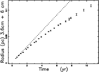
Fig. 1 : Radius in pc versus year of SN 1993J with vertical error bars. The em bands are $\lambda=3.6\,cm$ and $\lambda=6\,cm$. The data are extracted from Table 1 in Marcaide et al. 2009. The dotted line represents an expansion at a constant velocity.

The instantaneous velocity of expansion can be deduced from the following formula

$$v_{j}=\frac{r_{j+1}-r_{j}}{t_{j+1}-t_{j}}\quad,$$ (1)

where $r_{j}$ and $t_{j}$ denote the radius and the time at the position $j$. The uncertainty in the instantaneous velocity is found by implementing the error propagation equation (often called the law of errors of Gauss) when the covariant terms are neglected, see  Bevington, P. R. and Robinson, D. K. (2003)). Fig. 2 reports the instantaneous velocity aw well the relative uncertainty.

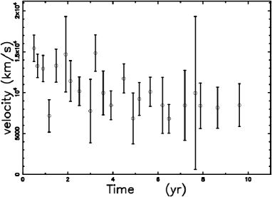
Fig. 2 : Instantaneous velocity of SN 1993J with uncertainty.

In particular, the observed instantaneous velocity decreases from $v=15437~{}\frac{km}{s}$ at $t=0.052$ yr to $v=8474~{}\frac{km}{s}$ at $t=10.53$ yr. We briefly recall that Fransson et al. (2005) quote an inner velocity from the shapes of the lines of $\approx 7000\frac{km}{s}$ and an outer velocity of $\approx 10000\frac{km}{s}$.

3 Classical case

This section reviews the free expansion , two simple laws of motion for the SNR and a new law of motion in the light of the classical physics.

3.1 The constant expansion velocity

The SNR expands at a constant velocity until the surrounding mass is of the order of the solar mass. This time , $t_{M}$ , is

$$t_{M}=186.45\,{\frac{\sqrt[3]{{\it M_{\sun}}}}{\sqrt[3]{{\it n_{0}}}{\it v_{10000}}}}\quad yr\quad,$$ (2)

where $M_{\sun}$ is the number of solar masses in the volume occupied by the SNR, $n_{0}$, the number density expressed in particles $\mathrm{cm}^{-3}$, and $v_{10000}$ the initial velocity expressed in units of $10000\,km/s$ , see McCray and Layzer (1987).

3.2 Two solutions

A first law of motion for the $SNR$ is the Sedov solution

$$R(t)=\left({\frac{25}{4}}\,{\frac{{\it E}\,{t}^{2}}{\pi\,\rho}}\right)^{1/5}\quad,$$ (3)

where $E$ is the energy injected into the process and $t$ is time, see Sedov (1959); McCray and Layzer (1987). Our astrophysical units are: time, ($t_{1}$), which is expressed in years; $E_{51}$, the energy in $10^{51}$ erg; $n_{0}$, the number density expressed in particles $\mathrm{cm}^{-3}$  (density $\rho=n_{0}$m, where m = 1.4$m_{\mathrm{H}}$). In these units, equation (3) becomes

$$R(t)\approx 0.313\,\sqrt[5]{{\frac{{\it E_{51}}\,{{\it t_{1}}}^{2}}{{\it n_{0}}}}}~{}{pc}\quad.$$ (4)

The Sedov solution scales as $t^{0.4}$. We are now ready to couple the Sedov phase with the free expansion phase

$$R(t)=\left\{\begin{array}[]{ll}0.0157\,{\it t}\,pc&\mbox{if $t\leq 2.5yr$ }\\ 0.0273\,\sqrt[5]{{{\it t}}^{2}}\,pc&\mbox{if $t>2.5yr$ ~{}.}\end{array}\right.$$ (5)

This two phases solution is obtained with the following parameters $M_{\sun}$ =1 , $n_{0}=1.127\,10^{5}$ , $E_{51}=0.567$ and Fig. 3 reports it’s temporal behavior as well the data. The quality of the simulation , $\epsilon_{q}$, can be obtained by a comparison of observed and simulated quantities:

$$\epsilon_{q}=(1-\frac{|(R_{\mathrm{pc,obs}}-R_{pc,\mathrm{num}})|}{R_{pc,\mathrm{obs}}})\cdot 100\,,$$ (6)

where $R_{pc,\mathrm{obs}}$ is the observed radius, in parsec and $R_{pc,\mathrm{num}}$ is the radius from our simulation in parsec. In the case of the two-phases simulation we have $\epsilon_{q}=65\%$ which is a low value in comparison with the other models here considered see Table 1.

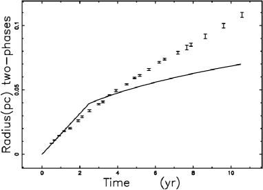
Fig. 3 : Theoretical radius as given by the two-phases solution with data as in Table 1 (full line), and astronomical data of SN 1993J with vertical error bars.

A second solution is connected with momentum conservation in the presence of a constant density medium, see Dyson, J. E. and Williams, D. A. (1997); Padmanabhan (2001); Zaninetti (2009). The astrophysical radius in pc as a function of time is

$$R(t)=\sqrt[4]{{{\it R_{0}}}^{3}\left(4.08\,10^{-6}\,{\it v_{1}}\,\left(t_{1}-t_{{0}}\right)+{\it R_{0}}\right)}\,pc\quad,$$ (7)

where $t_{1}$ and $t_{0}$ are times in years, $R_{0}$ is the radius in pc when $t_{1}=t_{0}$ and $v_{1}$ is the velocity in $\frac{1\,km}{s}$ units when $t_{1}=t_{0}$. The momentum solution in the presence of a constant density medium scales as $t^{0.25}$.

3.3 Momentum conservation with variable density

We assume that around the SNR the density of the interstellar medium (ISM) has the following two piecewise dependencies

$$\rho(R)=\left\{\begin{array}[]{ll}\rho_{0}&\mbox{if $R\leq R_{0}$ }\\ \rho_{0}(\frac{R_{0}}{R})^{d}&\mbox{if $R>R_{0}$ ~{}.}\end{array}\right.$$ (8)

In this framework, the density decreases as an inverse power law with an exponent $d$ that can be fixed from the observed temporal evolution of the radius, with $d=0$ meaning constant radius. The mass swept, $M_{0}$, in the interval $0\leq r\leq R_{0}$ is

$$M_{0}=\frac{4}{3}\,\rho_{{0}}\pi\,{R_{{0}}}^{3}\quad.$$ (9)

The mass swept, $M$, in the interval $0\leq r\leq R$ with $r\geq R_{0}$ is

$$M=-4\,{r}^{3}\rho_{{0}}\pi\,\left({\frac{R_{{0}}}{r}}\right)^{d}\left(d-3\right)^{-1}$$

$$+4\,{\frac{\rho_{{0}}\pi\,{R_{{0}}}^{3}}{d-3}}+\frac{4}{3}\,\rho_{{0}}\pi\,{R_{{0}}}^{3}\quad.$$ (10)

Momentum conservation requires that

$$Mv=M_{0}v_{0}\quad,$$ (11)

where $v$ is the velocity at $t$ and $v_{0}$ is the velocity at $t=t_{0}$. This formula is not invariant under Lorentz transformations and the initial velocity, $v_{0}$, can be greater than the velocity of light. The previous expression as a function of the radius is

$$\beta=\frac{{{\it r_{0}}}^{3}{\it\beta_{0}}\,\left(3-d\right)}{3\,{{\it r_{0}}}^{d}{R}^{3-d}-{{\it r_{0}}}^{3}d}\quad,$$ (12)

where $\beta_{0}$=$v_{0}/c_{l}$, $\beta$=$v/c_{l}$ and $c_{l}$ is the velocity of light. Here, we have introduced a relativistic notation for later use. In this differential equation of first order in $R$, the variables can be separated and an integration term-by-term gives the following nonlinear equation ${\mathcal{F}}_{NL}$

$${\mathcal{F}}_{NL}=\left(4{R_{{0}}}^{3}d-{R_{{0}}}^{3}{d}^{2}\right)R-3{R_{{0}}}^{d}{R}^{4-d}+{R_{{0}}}^{4}{d}^{2}$$

$$+12{R_{{0}}}^{3}v_{{0}}t+3{R_{{0}}}^{4}-4{R_{{0}}}^{4}d$$

$$+7{R_{{0}}}^{3}v_{{0}}d{\it t_{0}}+{R_{{0}}}^{3}v_{{0}}{d}^{2}t$$

$$-7{R_{{0}}}^{3}v_{{0}}dt-12{R_{{0}}}^{3}v_{{0}}{\it t_{0}}-{R_{{0}}}^{3}v_{{0}}{d}^{2}{\it t_{0}}=0\quad.$$ (13)

An approximate solution of ${\mathcal{F}}_{NL}(r)$ can be obtained assuming that $3R_{0}^{d}R^{4-d}$ $\gg$ $-(4R_{0}^{3}d-R_{0}^{3}d^{2})R$

$$R(t)=$$

$$({R_{{0}}}^{4-d}-\frac{1}{3}d{R_{{0}}}^{4-d}(4-d)$$

$$+\frac{1}{3}(4-d)v_{{0}}{R_{{0}}}^{3-d}(3-d)(t-t_{{0}}))^{\frac{1}{4-d}}\quad.$$ (14)

Up to now, the physical units have not been specified, pc for length and yr for time are perhaps an acceptable choice. With these units, the initial velocity $v_{{0}}$ is expressed in $\frac{pc}{yr}$ and should be converted into $\frac{km}{s}$; this means that $v_{{0}}=1.02\,10^{-6}v_{{1}}$ where $v_{{1}}$ is the initial velocity expressed in $\frac{km}{s}$.

The astrophysical version of the above equation in pc is

$$R(t)=$$

$$({R_{0}}^{4-d}-\frac{1}{3}d{R_{{0}}}^{4-d}(4-d)+3.402\,10^{-7}\times$$

$$\times(4-d)v_{{1}}{R_{{0}}}^{3-d}(3-d)(t_{1}-t_{{0}}))^{\frac{1}{4-d}}\,pc\quad,$$ (15)

where $t_{1}$ and $t_{0}$ are times in years, $R_{0}$ is the radius in pc at $t_{1}=t_{0}$ and $v_{1}$ is the velocity at $t_{1}=t_{0}$ in $\frac{km}{s}$.

4 Classical fits

The quality of the fits is measured by the merit function $\chi^{2}$

$$\chi^{2}=\sum_{j}\frac{(R_{th}-R_{obs})^{2}}{\sigma_{obs}^{2}}\quad,$$ (16)

where $R_{th}$, $R_{obs}$ and $\sigma_{obs}$ are the theoretical radius, the observed radius and the observed uncertainty respectively.

A first numerical analysis of the observed radius–time relationship of SN 1993J can be done by assuming a power law dependence of the type

$$R(t)=r_{p}t^{\alpha_{p}}\quad.$$ (17)

The two parameters $r_{p}$ and $\alpha_{p}$ can be found from the following logarithmic transformation

$$\ln(R(t))=\ln(r_{p})+\alpha_{p}\ln(t)\quad,$$ (18)

which can be written as

$$y=a_{LS}+b_{LS}x\quad.$$ (19)

The application of the least square method through the FORTRAN subroutine LFIT from Press et al. (1992) allows to find $a_{LS}$ ,$b_{LS}$ and the errors $\sigma_{a}$ and $\sigma_{b}$, see numerical values in Table 1. The error on $r_{p}$ is found by implementing the error propagation equation (often called law of errors of Gauss) when the covariant terms are neglected (see equation (3.14) in Bevington, P. R. and Robinson, D. K. (2003)),

$$\sigma_{r_{p}}=\exp(a)\sigma_{a}\quad,$$ (20)

and $\sigma_{\alpha_{p}}$ = $\sigma_{b}$. In this case, the velocity is

$$V(t)=r_{p}\,\alpha_{p}t^{(\alpha_{p}-1)}\quad.$$ (21)

Table 1 : Numerical values of the parameters of the fits and $\chi^{2}$. $N$ represents the number of free parameters and $\epsilon_{q}$ the quality of the simulation.

$\displaystyle\hskip 0.0pt{\begin{array}[]{cccc}\hline\cr\hline\cr\vskip 6.0pt\cr N&values&\chi^{2}&\epsilon_{q}\\ \vskip 6.0pt\cr\hline\cr\vskip 6.0pt\cr&power~{}law&&\\ \vskip 6.0pt\cr 2&\alpha_{p}=0.82\pm 0.0048&6364&98.54\%\\ \vskip 6.0pt\cr{}\hfil&r_{p}=(0.015\pm 0.00011)&&\\ \vskip 6.0pt\cr\hline\cr&piecewise&&\\ \vskip 6.0pt\cr 4&\alpha_{1}=0.83\pm 0.01&32&97.76\%\\ &\alpha_{2}=0.78\pm 0.0077;&{}\hfil&{}\hfil\\ \vskip 6.0pt\cr{}\hfil&r_{br}=0.05~{}{pc};t_{br}=4.10~{}{yr}&{}\hfil&{}\hfil\\ \vskip 6.0pt\cr\hline\cr&approximate~{}radius&&\\ \vskip 6.0pt\cr 4&d=2.54;r_{0}=0.019~{}{pc};&7186&96.95\%\\ \vskip 6.0pt\cr{}\hfil&t_{0}=0.249~{}{yr};v_{0}=100000\frac{km}{s}&{}\hfil&{}\hfil\\ \vskip 6.0pt\cr\hline\cr{}\hfil&nonlinear~{}radius&&\\ \vskip 6.0pt\cr 4&d=2.93;r_{0}=0.019~{}{pc};&276&93.3\%\\ \vskip 6.0pt\cr&t_{0}=0.249~{}{yr};v_{0}=100000\frac{km}{s}&{}\hfil&{}\hfil\\ \vskip 6.0pt\cr\hline\cr&relativistic~{}radius&&\\ \vskip 6.0pt\cr 4&d=2.54;r_{0}=0.0045~{}{pc};&5557&93.05\%\\ \vskip 6.0pt\cr{}\hfil&t_{0}=0.249~{}{yr};\beta_{0}=0.333&{}\hfil&{}\hfil\\ \vskip 6.0pt\cr\hline\cr&relativistic~{}pressure~{}radius&&\\ \vskip 6.0pt\cr 5&d=0.89;r_{0}=0.00072~{}{pc}&1844&99.93\%\\ \vskip 6.0pt\cr{}\hfil&f=10^{-5}&{}\hfil&{}\hfil\\ \vskip 6.0pt\cr{}\hfil&t_{0}=0.249~{}{yr};\beta_{0}=0.333&{}\hfil&{}\hfil\\ \vskip 6.0pt\cr\hline\cr\hline\cr\end{array}}$

A second numerical analysis can be done by assuming a piecewise function as in Fig. 4 of Marcaide et al. (2009)

$$R(t)=\left\{\begin{array}[]{ll}r_{br}(\frac{t}{t_{br}})^{\alpha_{1}}&\mbox{if $t\leq t_{br}$ }\\ r_{br}(\frac{t}{t_{br}})^{\alpha_{2}}&\mbox{if $t>t_{br}$. }\end{array}\right.$$ (22)

This type of fit requires the determination of four parameters, i.e., $t_{br}$, the break time, $r_{br}$ the radius of expansion at $t=t_{br}$ and the exponents of the two phases are $alpha_{1}$ and $alpha_{2}$. The two-regime fit can be visualized in Fig. 4 and Table 1 reports the four parameters.

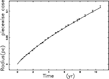
Fig. 4 : Theoretical radius as given by the two-regime fit represented by equation (22) with data as in Table 1 (full line), and astronomical data of SN 1993J with vertical error bars.

A third type of fit can be done by adopting the approximate radius as given by equation (15); Fig. 5 reports a fit of this type.

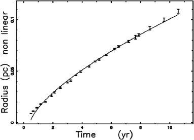
Fig. 5 : Theoretical radius as given by the approximate radius, equation (15), with data as in Table 1 (full line). The astronomical data of SN 1993J are represented with vertical error bars.

A fourth type of fit implements the nonlinear equation (13); the four roots can be found with the FORTRAN subroutine ZRIDDR from Press et al. (1992); Fig. 6 reports a fit of this type.

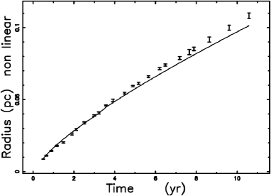
Fig. 6 : Theoretical radius as obtained by the solution of the nonlinear equation (13) (full line), data as in Table 1. The astronomical data of SN 1993J are represented with vertical error bars.

5 Relativistic case

The relativistic analysis is split in two.

1. The relativistic mechanics case in which the temperature effects are ignored and the thin layer approximation is used.

2. The case of relativistic hydrodynamics in which the pressure is considered and the velocity is found from momentum conservation.

5.1 Relativistic mechanics

Newton’s law in special relativity, after Einstein (1905), is:

$$F=\frac{dp}{dt}=\frac{d}{dt}(mV)\quad,$$ (23)

with

$$m=\frac{m_{r}}{\sqrt{1-\frac{v^{2}}{c_{l}^{2}}}}\quad,$$ (24)

where $F$ is the force, $p$ is the relativistic momentum, $m$ is the relativistic mass, $m_{r}$ is the rest-mass, $v$ is the velocity and $c_{l}$ is the velocity of light, see equation (7.16) in French, A.P. (1968). In the case of the relativistic expansion of a shell in which all the swept material resides at two different points, denoted by radius $R$ and radius $R_{0}$, the previous equation gives:

$$M\frac{\beta}{\sqrt{1-\beta^{2}}}=M_{0}\frac{\beta_{0}}{\sqrt{1-\beta_{0}^{2}}}\quad,$$ (25)

where $\beta_{0}$=$v_{0}/c_{l}$, $\beta$=$v/c_{l}$, $M$ is the rest mass swept between 0 and $R$ and $M_{0}$ is the rest mass swept between 0 and $R_{0}$. This formula is invariant under Lorentz transformations and the initial velocity, $v_{0}$, cannot be greater than the velocity of light. Assuming a spatial dependence of the ISM as given by formula (8), relativistic conservation of momentum gives

$$\frac{-4\,\rho\,\pi\,\left(3\,{r}^{3}\left({\frac{{\it r_{0}}}{r}}\right)^{d}-{{\it r_{0}}}^{3}d\right)\beta}{3\,\left(-3+d\right)\sqrt{1-{\beta}^{2}}}=\frac{4\,\rho\,\pi\,{{\it r_{0}}}^{3}{\it\beta_{0}}}{3\,\sqrt{1-{{\it\beta_{0}}}^{2}}}\quad.$$ (26)

According to the previous equation, $\beta$ is

$$\beta=\frac{-\left(-3+d\right){\it\beta_{0}}\,{{\it r_{0}}}^{3}}{\sqrt{D_{\beta}}}$$ (27)

$$with~{}D_{\beta}=9\,{R_{{0}}}^{6}{\beta_{{0}}}^{2}-6\,{R_{{0}}}^{6}{\beta_{{0}}}^{2}d$$

$$+9\,{r}^{6-2\,d}{R_{{0}}}^{2\,d}$$

$$-6\,{r}^{3-d}{R_{{0}}}^{d+3}d+{R_{{0}}}^{6}{d}^{2}$$

$$-9\,{\beta_{{0}}}^{2}{r}^{6-2\,d}{R_{{0}}}^{2\,d}+6\,{\beta_{{0}}}^{2}{r}^{3-d}{R_{{0}}}^{d+3}d\quad.$$

In this differential equation of first order in $r$, the variables can be separated and the integration can be expressed as

$$\int_{R_{0}}^{R}\sqrt{D_{\beta}}dR=c\left(3-d\right)\beta_{{0}}{R_{{0}}}^{3}\left(t-t_{{0}}\right)\quad.$$ (28)

The integral of the previous equation can be performed analytically only in the cases $d=0$, $d=1$ and $d=2$, but we do not report the result because we are interested in a variable value of $d$. The integral can be easily evaluated from a theoretical point of view using the subroutine QROMB from Press et al. (1992). The numerical result is reported in Fig. 7 and the input data in Table 1.

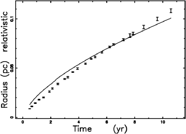
Fig. 7 : Theoretical radius as obtained by the solution of the relativistic-mechanics equation (28) (full line), data as in Table 1. The astronomical data of SN 1993J are represented with vertical error bars.

The behavior of relativistic and classical velocities are reported in Fig. 8.

Fig. 8 : Theoretical relativistic-mechanics velocity as given by equation (27) (dashed line), theoretical classical velocity as given by equation (12) (full line) and instantaneous velocity of SN 1993J with uncertainty.

5.2 Relativistic hydrodynamics

A relativistic flow on flat space time is described by the energy–momentum tensor, $T^{\mu\nu}$,

$$T^{\mu\nu}=wu^{\mu}u^{\nu}-pg^{\mu\nu}\quad,$$ (29)

where $u^{\mu}$ is the 4-velocity, and the Greek index varies from 0 to 3, $w$ is the enthalpy for unit volume, $p$ is the pressure and $g^{\mu\nu}$ the inverse metric of the manifold Weinberg (1972); Landau (1987); Hidalgo and Mendoza (2005); Gourgoulhon (2006). Momentum conservation in the presence of velocity, $v$, along the radial direction states that

$$(w(\frac{v}{c_{l}})^{2}\frac{1}{1-\frac{v^{2}}{c_{l}^{2}}}+p)A=cost\quad,$$ (30)

where $A(r)$ is the considered surface area, which is perpendicular to the motion. The enthalpy per unit volume is

$$w=c_{l}^{2}\rho+p\quad,$$ (31)

where $\rho$ is the density, and $c_{l}$ is the velocity of light. The reader may be puzzled by the $\gamma^{2}$ factor in equation (30), where $\gamma^{2}=\frac{1}{1-\frac{v^{2}}{c_{l}^{2}}}$. However it should be remembered that $w$ is not an enthalpy, but an enthalpy per unit volume: the extra $\gamma$ factor arises from ‘length contraction’ in the direction of motion Gourgoulhon (2006). We continue assuming

$$p=\frac{1}{3}f\rho{c_{l}}^{2}\quad,$$ (32)

where $f$ is a parameter which has the range $0\leq f\leq 1$ and is supposed to be constant during the expansion, see formula (2.10.26) in Weinberg (1972) for a hot extremely relativistic gas. The previous equation (30) becomes

$$\left({\frac{\left({c_{l}}^{2}\rho+\frac{1}{3}\,f\rho\,{c_{l}}^{2}\right){\beta}^{2}}{1-{\beta}^{2}}}+\frac{1}{3}\,f\rho\,{c_{l}}^{2}\right)A=constant\,.$$ (33)

The density is supposed to vary during the expansion as

$$\rho=\rho_{0}(\frac{R_{0}}{R})^{d}\quad,$$ (34)

where $\rho_{0}$ is the density at $R=R_{0}$. In two surfaces of the expansion we have:

$$-\left({\frac{R_{{0}}}{R}}\right)^{d}{R}^{2}{\beta}^{2}\left(-1+{\beta}^{2}\right)^{-1}$$

$$-1/3\,\left({\frac{R_{{0}}}{R}}\right)^{d}{R}^{2}f\left(-1+{\beta}^{2}\right)^{-1}$$

$$+{\frac{{R_{{0}}}^{2}{\beta_{{0}}}^{2}}{-1+{\beta_{{0}}}^{2}}}+1/3\,{\frac{{R_{{0}}}^{2}f}{-1+{\beta_{{0}}}^{2}}}=0\quad.$$ (35)

The positive solution of the second degree equation is:

$$\beta=\frac{N}{D}$$ (36)

$$N=-(-9\,{R_{{0}}}^{d+2}{R}^{-d+2}{\beta_{{0}}}^{4}+6\,{R_{{0}}}^{2\,d}{R}^{-2\,d+4}{\beta_{{0}}}^{2}f$$

$$-3\,{R_{{0}}}^{2\,d}{R}^{-2\,d+4}{\beta_{{0}}}^{4}f$$

$$-6\,{R_{{0}}}^{d+2}{R}^{-d+2}{\beta_{{0}}}^{2}f+9\,{R_{{0}}}^{d+2}{R}^{-d+2}{\beta_{{0}}}^{2}$$

$$-3\,{R_{{0}}}^{2\,d}{R}^{-2\,d+4}f+3\,{R_{{0}}}^{d+2}{R}^{-d+2}f$$

$$+9\,{R_{{0}}}^{4}{\beta_{{0}}}^{4}+3\,{R_{{0}}}^{d+2}{\beta_{{0}}}^{4}{R}^{-d+2}f+6\,{R_{{0}}}^{4}{\beta_{{0}}}^{2}f$$

$$-{R_{{0}}}^{d+2}{f}^{2}{R}^{-d+2}+{R_{{0}}}^{d+2}{f}^{2}{R}^{-d+2}{\beta_{{0}}}^{2}+{R_{{0}}}^{4}{f}^{2})^{\frac{1}{2}}$$

$$D=3\,{R_{{0}}}^{d}{R}^{-d+2}{\beta_{{0}}}^{2}$$

$$-3\,{R_{{0}}}^{d}{R}^{-d+2}-3\,{R_{{0}}}^{2}{\beta_{{0}}}^{2}-{R_{{0}}}^{2}f\quad.$$

The equation of motion is

$$\int_{R_{0}}^{R}\frac{D}{N}dR=c\left(t-t_{{0}}\right)\quad.$$ (37)

The integral is evaluated using the subroutine QROMB from Press et al. (1992). The numerical results are reported in Figs 9 and 10.

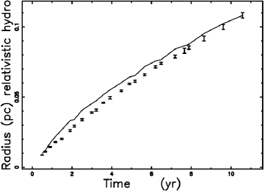
Fig. 9 : Theoretical radius as obtained by the solution of the relativistic-hydrodynamics equation (37) (full line) and data as in Table 1 with uncertainty.

Fig. 10 reports the decrease of the relativistic velocity.

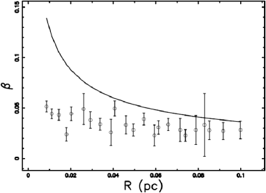
Fig. 10 : Theoretical relativistic-hydrodynamics velocity with pressure as given by equation (36) (full line), and instantaneous velocity of SN 1993J with uncertainty.

6 How the image is formed

In this section, the existing knowledge about adiabatic and synchrotron losses, the acceleration of particles by the Fermi II mechanism, , 3D mathematical diffusions with constant diffusion coefficients and the rim model with constant density are reviewed and applied to SN 1993J . A new example of a 1D random walk with a step length equal to the relativistic electron gyro-radius is also reported. A new simple model for the temporal evolution of the flux densities is introduced.

6.1 Acceleration and losses

6.1.1 Adiabatic losses

An ultrarelativistic gas which experiences an expansion loses energy at the rate

$$-(\frac{dE}{dt})=\frac{1}{3}(\nabla\cdot{\bf v})E\quad,$$ (38)

where $E$ is the energy and $\nabla\cdot{\bf v}$ is the divergence of the expansion velocity, see formula (11.27) in Longair (1994). A simple expression for $\nabla\cdot{\bf v}$ can be found from the power law model, see equations (17) and (21)

$$\nabla\cdot{\bf v}=\frac{{R}^{{\frac{\alpha-1}{\alpha}}}{{\it r_{p}}}^{\frac{1}{\alpha}}\left(3\,\alpha-1\right)}{R}\quad,$$ (39)

where $R$ is the temporary radius of the expansion and $r_{p}$ and $\alpha$ are reported in Table 1. The lifetime, $\tau_{ad}$, of an ultrarelativistic electron for adiabatic losses is

$$\tau_{ad}=\frac{E}{\frac{dE}{dt}}=344.39\,R^{1.22}\,yr\quad,$$ (40)

when the radius $R$ is expressed in pc. During the ten years of observed expansion, the radius of SN 1993J has grown from $\approx$ 0.01 pc to $\approx$ 0.1 pc and therefore the time scale of adiabatic losses has increased from $\approx$ 1.25 yr to $\approx$ 20.7 yr.

6.1.2 Synchrotron losses

An electron which loses its energy due to synchrotron radiation has a lifetime $\tau_{r}$, where

$$\tau_{r}\approx\frac{E}{P_{r}}\approx 500E^{-1}H^{-2}sec\quad,$$ (41)

$E$ is the energy in ergs, $H$ the magnetic field in Gauss, and $P_{r}$ is the total radiated power, see formula (1.157) in Lang (1999).

The energy is connected to the critical frequency, see formula (1.154) in Lang (1999), as

$$\nu_{c}=6.266\times 10^{18}HE^{2}~{}Hz\quad.$$ (42)

The lifetime, $\tau_{syn}$, for synchrotron losses is

$$\tau_{syn}=39660\,{\frac{1}{H\sqrt{H\nu}}}\,yr\quad.$$ (43)

The time-scale of synchrotron losses is shorter than that of the adiabatic losses if the following inequality is verified

$$\nu>\frac{1.572\,10^{9}}{H^{3}\,\tau_{ad}^{2}}\quad Hz\quad,$$ (44)

where $H$ is expressed in Gauss and $\tau_{ad}$ in years. The previous equation can also be expressed as

$$H>1162.98\,{\frac{1}{\sqrt[3]{{\it\nu}}{{\it t_{ad}}}^{2/3}}}Gauss\quad,$$ (45)

that is the magnetic field at which the synchrotron losses prevails on the adiabatic losses and Fig. 11 reports the numerical values of the transition.

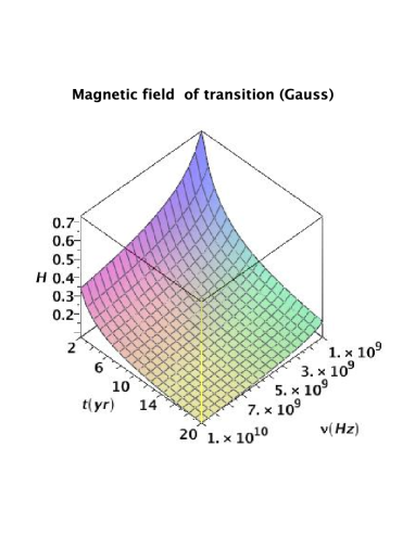
Fig. 11 : Magnetic field in Gauss over which the synchrotron losses prevail on the adiabatic losses.

6.1.3 Particle acceleration

Following Fermi (1949, 1954), the gain in energy $\Delta E$ of a particle which spirals around a line of force is proportional to its energy, $E$,

$$\Delta E=B^{2}E\quad,$$ (46)

where $B=u/c_{l}$ , see formula (3) in Fermi (1949). The continuous form is

$$\frac{dE}{dt}=\frac{E}{\tau}\quad,$$ (47)

where $\tau$ is the typical time-scale. The probability, $P(t)$ , that the particle remains in the reservoir for a period greater than $t$ is now introduced,

$$P(t)=e^{-\frac{t}{T}}\quad,$$ (48)

where $T$ is the time of escape from the considered region. The resulting probability density, $N(E)$, is

$$N(E)=\frac{\tau}{E_{0}}(\frac{E}{E_{0}})^{-\gamma_{f}}\quad,$$ (49)

where $E_{0}$ is the initial energy and

$$\gamma_{f}=1+\frac{\tau}{T}\quad.$$ (50)

Equation (49) can be written as

$$N(E)=K\;E^{-\gamma_{f}}\quad,$$ (51)

where $K=\frac{\tau}{{E_{0}}^{-\gamma_{f}+1}}$ . A power law spectrum in the particle energy has now been obtained. In Fermi II processes, the typical time-scale, $\tau_{II}$, when the particle stays in the accelerating region a time greater than $T$ is

$$\frac{1}{\tau_{II}}=\frac{4}{3}(\frac{u^{2}}{c_{l}^{2}})(\frac{c_{l}}{L})\quad,$$ (52)

where $u$ is the velocity of the accelerating cloud and $L$ is the mean free path between clouds, see formula after (4.439) in Lang (1999). The mean free path between the accelerating clouds in the Fermi II mechanism can be found from the following inequality:

$$\tau_{II}<\tau_{sync}\quad,$$ (53)

or

$$L<1.723\,10^{5}\,\frac{\beta^{2}}{H\,\sqrt{H\,\nu}}\quad pc\quad.$$ (54)

As an example, inserting $\beta=2.82\,10^{-2}$ (value of velocity at $\approx 0.1$ pc of SN 1993J ), $\nu=1.5GHz$ and $H=65.1~{}Gauss$ (Table 1 in Marti-Vidal et al. (2010)) we obtain

$$L<6.76\,10^{-6}\quad pc\quad.$$ (55)

This model of acceleration can work in the rim model with constant density of emitting particles, see Section 6.4. In this case the thickness of the emitting region is $b-a$=0.035 pc which means that an high number of collisions can be done. In Fermi II process the energy increases exponentially with time

$$E(t)=E_{0}\exp(t/\tau)\quad,$$ (56)

see , equation (3) in Fermi (1954). The effect of the synchrotron losses on the energy of the electron during the various collisions and the consequent equilibrium energy has been analyzed in Zaninetti and Siah (1988). The strong shock accelerating mechanism, named Fermi I, was later introduced by Bell (1978, 1978) and produces an increases in energy of the particle of the type

$$\Delta E=\frac{u}{c_{l}}E\quad,$$ (57)

where $u$ is the velocity of the shock, see formula (21.20) in Longair (1994). This process allows to predict a probability density in the energy of the accelerated particles of the type $N(E)\propto E^{-2}$. In our case can be considered the process which accelerates the particles before they start to diffuse from the shock , see Section 6.3 and 6.4. A modern review of the two Fermi mechanisms can be found in Kulsrud (2005); Somov (2006); Dermer and Menon (2009).

6.2 The transfer equation

The transfer equation in the presence of emission only, see for example Rybicki and Lightman (1991) or Hjellming, R. M. (1988), is

$$\frac{dI_{\nu}}{ds}=-k_{\nu}\rho I_{\nu}+j_{\nu}\rho\quad,$$ (58)

where $I_{\nu}$ is the specific intensity, $s$ is the line of sight, $j_{\nu}$ is the emission coefficient, $k_{\nu}$ is a mass absorption coefficient, $\rho$ is the density of mass at position $s$ and the index $\nu$ denotes the frequency of emission of interest. The solution to equation (58) is

$$I_{\nu}(\tau_{\nu})=\frac{j_{\nu}}{k_{\nu}}(1-e^{-\tau_{\nu}(s)})\quad,$$ (59)

where $\tau_{\nu}$ is the optical depth at frequency $\nu$

$$d\tau_{\nu}=k_{\nu}\rho ds\quad.$$ (60)

The volume emissivity (power per unit frequency interval per unit volume per unit solid angle) of the ultrarelativistic radiation from a group of electrons, according to Lang (1999), is

$$\epsilon(\nu)=\int P(\nu)N(E)dE\quad,$$ (61)

where $P(\nu)$ is the total power radiated per unit frequency interval by one electron and $N(E)dE$ is the number of electrons per unit volume, per unit solid angle along the line of sight that are moving in the direction of the observer and whose energies lie in the range $E$ to $E+dE$. In the case of a power law spectrum,

$$N(E)dE=KE^{-\gamma_{f}}\quad,$$ (62)

where $K$ is a constant. The value of the constant $K$ can be found by assuming that the probability density function for the relativistic energy is of Pareto type as defined in Evans, Hastings, and Peacock (2000)

$$f(x;a,c_{p})={c_{p}a^{c_{p}}}{x^{-(c_{p}+1)}}\quad,$$ (63)

with $c_{p}~{}>0$. In our case, $c_{p}=\gamma_{f}-1$ and $a=E_{min}$, where $E_{min}$ is the minimum energy. We can now extract

$$K=N_{0}(\gamma_{f}-1)E_{min}^{\gamma_{f}-1}\quad,$$ (64)

where $N_{0}$ is the total number of relativistic electrons per unit volume, here assumed to be approximately equal to the matter number density. The previous formula can also be expressed as

$$K=\frac{\rho}{1.4\,m_{\mathrm{H}}}(\gamma_{f}-1)E_{min}^{\gamma_{f}-1}\quad,$$ (65)

where $m_{H}$ is the mass of hydrogen. The emissivity of the ultrarelativistic synchrotron radiation from a homogeneous and isotropic distribution of electrons whose $N(E)$ is given by equation (62) is, according to Lang (1999),

$$j_{\nu}\rho=$$ (66)

$$\approx 0.933\times 10^{-23}\alpha(\gamma_{f})KH_{\perp}^{(\gamma_{f}+1)/2}\times$$

$$\times\bigl{(}\frac{6.26\times 10^{18}}{\nu}\bigr{)}^{(\gamma_{f}-1)/2}$$

$$erg\,sec^{-1}cm^{-3}Hz^{-1}rad^{-2}\quad,$$

where $\nu$ is the frequency and $\alpha(\gamma_{f})$ is a slowly varying function of $\gamma_{f}$ which is of the order of unity and is given by

$$\alpha(\gamma_{f})=$$

$$2^{(\gamma_{f}-3)/2}\frac{\gamma_{f}+7/3}{\gamma_{f}+1}\Gamma\bigl{(}\frac{3\gamma_{f}-1}{12}\bigr{)}\Gamma\bigl{(}\frac{3\gamma_{f}+7}{12}\bigr{)}\quad,$$ (67)

for $\gamma_{f}\geq\frac{1}{2}$.

We now continue to analyze the case of an optically thin layer in which $\tau_{\nu}$ is very small (or $k_{\nu}$ is very small) and where the the density $\rho$ is substituted for the concentration $C(s)$ of relativistic electrons

$$j_{\nu}\rho=K_{e}C(s)\quad,$$ (68)

where $K_{e}$ is a constant function of the energy power law index, magnetic field and frequency of e.m. emission. The intensity is now

$$I_{\nu}(s)=K_{e}\int_{s_{0}}^{s}C(s\prime)ds\prime\quad\mbox{Optically thin layer}\quad.$$ (69)

The increase in brightness is proportional to the concentration integrated along the line of sight. In numerical experiments, the concentration is memorized on the visitation-grid ${\mathcal{S}}$ and the intensity is

$${\it I}\/(i,j)=\sum_{k}\triangle\,s\times{\mathcal{S}}(i,j,k)$$ (70)

$$\quad\mbox{Optically thin layer}\quad,$$

where $\triangle$s is the spatial interval between the various values and the sum is performed over the interval of existence of index $k$. The theoretical flux density is then obtained by integrating the intensity at a given frequency over the solid angle of the source. In order to deal with the transition to the optically thick case, the intensity is given by

$${\it I}\/(i,j)=\frac{1}{K_{a}}(1-\exp(-K_{a}\sum_{k}\triangle\,s\times{\mathcal{S}}(i,j,k)))$$ (71)

$$\quad\mbox{Thin $\longmapsto$ Thick }\quad,$$

where $K_{a}$ is a constant that represents the absorption. Considering the Taylor expansion of the last formula (71), equation (70) is obtained.

6.3 3D diffusion from a spherical source

Once the concentration, $C$, and diffusion coefficient, $D$, are introduced, Fick’ s law in three dimensions is

$$\frac{\partial C}{\partial t}=D\nabla^{2}C\quad.$$ (72)

Under steady-state conditions,

$$D\nabla^{2}C=0\quad.$$ (73)

The concentration rises from 0 at r=a to a maximum value $C_{m}$ at r=b and then falls again to 0 at r=c. The solution of equation (73) is

$$C(r)=A+\frac{B}{r}\quad,$$ (74)

where $A$ and $B$ are determined by the boundary conditions,

$$C_{ab}(r)=C_{{m}}\left(1-{\frac{a}{r}}\right)\left(1-{\frac{a}{b}}\right)^{-1}\quad a\leq r\leq b\quad,$$ (75)

and

$$C_{bc}(r)=C_{{m}}\left({\frac{c}{r}}-1\right)\left({\frac{c}{b}}-1\right)^{-1}\quad b\leq r\leq c\quad.$$ (76)

These solutions can be found in Berg (1993) or in Crank (1979). Fig. 12 shows a spherical shell source of radius $b$ between a spherical absorber of radius $a$ and a spherical absorber of radius $c$.

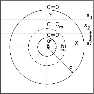
Fig. 12 : The spherical source is represented by the dashed line and the two absorbing boundaries by full lines. The observer is situated along the $x$ direction, and three lines of sight are indicated. Adapted from Fig. 3.1 in Berg (1993).

The concentration rises from 0 at r=a to a maximum value $C_{m}$ at r=b and then falls again to 0 at r=c. The concentrations to be used are formulas (75) and (76) once $r=\sqrt{x^{2}+y^{2}}$ is imposed; these two concentrations are inserted in formula (59) which represents the transfer equation. The geometry of the phenomenon fixes three different zones ($0-a,a-b,b-c$) for the variable $y$, see Zaninetti (2007); the first segment, $I^{I}(y)$, is

$$I^{I}(y)=$$

$$2{\frac{b{\it C_{m}}\sqrt{{a}^{2}-{y}^{2}}}{-b+a}}-2{\frac{b{\it C_{m}}a\ln\left(\sqrt{{a}^{2}-{y}^{2}}+a\right)}{-b+a}}$$

$$-2{\frac{b{\it C_{m}}\sqrt{{b}^{2}-{y}^{2}}}{-b+a}}+2{\frac{b{\it C_{m}}a\ln\left(\sqrt{{b}^{2}-{y}^{2}}+b\right)}{-b+a}}$$

$$+2{\frac{b{\it C_{m}}c\ln\left(\sqrt{{b}^{2}-{y}^{2}}+b\right)}{-c+b}}-2{\frac{b{\it C_{m}}\sqrt{{b}^{2}-{y}^{2}}}{-c+b}}$$

$$-2{\frac{b{\it C_{m}}c\ln\left(\sqrt{{c}^{2}-{y}^{2}}+c\right)}{-c+b}}+2{\frac{b{\it C_{m}}\sqrt{{c}^{2}-{y}^{2}}}{-c+b}}$$ (77)

$$~{}0\leq y<a\quad.$$

The second segment, $I^{II}(y)$, is

$$I^{II}(y)=-{\frac{b{\it C_{m}}a\ln\left({y}^{2}\right)}{-b+a}}-2{\frac{b{\it C_{m}}\sqrt{{b}^{2}-{y}^{2}}}{-b+a}}$$

$$+2{\frac{b{\it C_{m}}a\ln\left(\sqrt{{b}^{2}-{y}^{2}}+b\right)}{-b+a}}$$

$$+2{\frac{b{\it C_{m}}c\ln\left(\sqrt{{b}^{2}-{y}^{2}}+b\right)}{-c+b}}$$

$$-2{\frac{b{\it C_{m}}\sqrt{{b}^{2}-{y}^{2}}}{-c+b}}-2{\frac{b{\it C_{m}}c\ln\left(\sqrt{{c}^{2}-{y}^{2}}+c\right)}{-c+b}}$$

$$+2{\frac{b{\it C_{m}}\sqrt{{c}^{2}-{y}^{2}}}{-c+b}}$$ (78)

$$a\leq y<b\quad.$$

The third segment, $I^{III}(y)$, is

$$I^{III}(y)=$$

$${\frac{b{\it C_{m}}c\ln\left({y}^{2}\right)}{-c+b}}-2{\frac{b{\it C_{m}}c\ln\left(\sqrt{{c}^{2}-{y}^{2}}+c\right)}{-c+b}}$$

$$+2{\frac{b{\it C_{m}}\sqrt{{c}^{2}-{y}^{2}}}{-c+b}}$$

$$b\leq y<c\quad.$$ (79)

The profile of ${\it I}$ made up of the three segments (77), (78) and (79), can be calibrated against the real data of SN 1993J and an acceptable match can be achieved by adopting the parameters reported in Table 2.

Table 2 : Simulation of SN 1993J by 3D diffusion, optically thin case

$\displaystyle\hskip 0.0pt{\begin{array}[]{lll}\hline\cr\hline\cr\vskip 6.0pt\cr symbol&meaning&value\\ \vskip 6.0pt\cr\hline\cr\vskip 6.0pt\cr a&radius~{}internal~{}sphere&1.76(mas)\\ \vskip 6.0pt\cr b&radius~{}shock&2.2(mas)\\ \vskip 6.0pt\cr c&radius~{}external~{}sphere&5.0(mas)\\ \vskip 6.0pt\cr\frac{I_{limb}}{I_{center}}&ratio~{}observed~{}intensities&1.7926\\ \vskip 6.0pt\cr\frac{I_{max}}{I(y=0)}&ratio~{}theoretical~{}intensities&1.7927\\ \vskip 6.0pt\cr\hline\cr\hline\cr\end{array}}$

The theoretical intensity can therefore be plotted as a function of the distance from the center, see Fig. 13, or as a contour map, see Fig. 14.

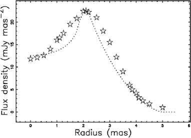
Fig. 13 : Cross-section of the mathematical intensity ${\it I}$ (formulas (77), (78) and (79)), through the center (dotted line) of SN 1993J and real data (empty stars), $\chi^{2}$ = 100.49 The real data made on day 1889 after the explosion have been extracted by the author from Fig. 3 of Marcaide et al. (2009). Parameters as in Table 2.

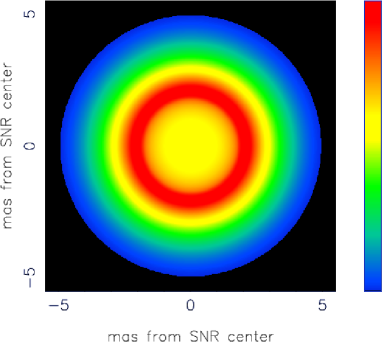
Fig. 14 : Contour map of ${\it I}$ adjusted to simulate SN 1993J . Parameters as in Table 2.

The position of the minimum of ${\it I}$ is at $y=0$ and the position of the maximum is situated in the region $a\leq y<b$, or more precisely at:

$$y={\frac{\sqrt{-\left(b-2\,a+c\right)a\left(ab-2\,bc+ac\right)}}{b-2\,a+c}}\quad.$$ (80)

This means that the maximum emission is not at the position of the shock, identified here as $b$, but shifted a little towards the center; see Fig. 15.

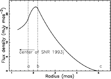
Fig. 15 : Cross-section through the mathematical intensity ${\it I}$ towards the edge of SN 1993J . The three parameters which characterize the expanding PN, a , b and c, are reported. Parameters as in Table 2.

The ratio between the theoretical maximum intensity, $I_{max}$, as given by formula (80), and minimum intensity ($y=0$) is complex and is reported in formulas (74-76) in Zaninetti (2007). The observed ratio as well as the theoretical ratio are reported in Table 2.

The effect of absorption is easily evaluated by applying formula (71) and fixing the value of $K_{a}$. The result is shown in Fig. 16.

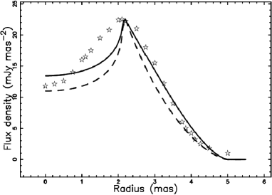
Fig. 16 : Cross-section through the mathematical intensity ${\it I}$ (formulas (77), (78) and (79)), in the optically thin case (dashed line, $\chi^{2}=237.3$), and optically thick case (full line, $\chi^{2}=84.7$) and real data (empty stars). Parameters as in Table 3.

Table 3 : Simulation of SN 1993J with 3D diffusion, optically thick case with $K_{a}=0.2$.

$\displaystyle\hskip 0.0pt{\begin{array}[]{llc}\hline\cr\hline\cr\vskip 6.0pt\cr symbol&meaning&value\\ \vskip 6.0pt\cr\hline\cr\vskip 6.0pt\cr a&radius~{}internal~{}sphere&2.01(mas)\\ \vskip 6.0pt\cr b&radius~{}of~{}shock&2.2(mas)\\ \vskip 6.0pt\cr c&radius~{}external~{}sphere&5.0(mas)\\ \vskip 6.0pt\cr\frac{I_{limb}}{I_{center}}&ratio~{}observed~{}intensities&1.7926\\ \vskip 6.0pt\cr\frac{I_{max}}{I(y=0)}&ratio~{}optically~{}thin~{}case&2.0491\\ \vskip 6.0pt\cr\frac{I_{max}}{I(y=0)}&ratio~{}optically~{}thick~{}case&1.6741\\ \vskip 6.0pt\cr\hline\cr\hline\cr\end{array}}$

6.4 The rim model with constant density

We assume that the number density of ultrarelativistic electrons $C$ is constant and in particular rises from 0 at $r=a$ to a maximum value $C_{m}$ , remains constant up to $r=b$ and then falls again to 0, see Section 5.2 in Zaninetti (2009). The length of sight , when the observer is situated at the infinity of the $x$-axis , is the locus parallel to the $x$-axis which crosses the position $y$ in a Cartesian $x-y$ plane and terminates at the external circle of radius $b$. The locus length is

$$l_{0a}=2\times(\sqrt{b^{2}-y^{2}}-\sqrt{a^{2}-y^{2}})\quad;0\leq y<a$$

$$l_{ab}=2\times(\sqrt{b^{2}-y^{2}})\quad;a\leq y<b\quad.$$ (81)

When the number density of ultrarelativistic electrons $C_{m}$ is constant between two spheres of radius $a$ and $b$ the intensity of radiation is

$$I_{0a}=$$

$$C_{m}\times 2\times(\sqrt{b^{2}-y^{2}}-\sqrt{a^{2}-y^{2}})\quad;0\leq y<a$$ (82)

$$I_{ab}=C_{m}\times 2\times(\sqrt{b^{2}-y^{2}})\quad;a\leq y<b\quad.$$ (83)

The ratio between the theoretical intensity at the maximum , $(y=a)$ , and at the minimum , ($y=0$) , is given by

$$\frac{I(y=a)}{I(y=0)}=\frac{\sqrt{b^{2}-a^{2}}}{b-a}\quad.$$ (84)

The parameter $b$ is identified with the external radius of the SNR. The parameter $a$ can be found from the following formula

$$a=\frac{b\left((\frac{I(y=a)}{I(y=0)})_{obs}^{2}-1\right)}{\left((\frac{I(y=a)}{I(y=0)})_{obs}^{2}+1\right)}\quad,$$ (85)

where $(\frac{I(y=a)}{I(y=0)})_{obs}$ is the observed ratio between maximum intensity at the rim and intensity at the center. A cut in the theoretical intensity is reported in Figure 17.

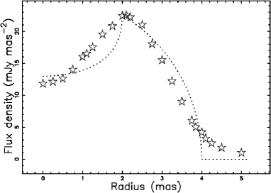
Fig. 17 : Cut of the mathematical intensity ${\it I}$ of the rim model ( equation (83)) through the center (dotted line) of SN 1993J and real data (empty stars). The parameters are $a=2$ mas , $b=4$ mas , $\frac{I(y=a)}{I(y=0)}$=1.73 and $\chi^{2}$ = 125.19.

6.5 1D diffusion

The Fick equation in 1D with a constant diffusion coefficient, see Crank (1979), is

$$\frac{d^{2}C}{dr^{2}}=0\quad.$$ (86)

The general solution to equation (86) is

$$C(r)=A+Br\quad.$$ (87)

The boundary conditions give

$$C(r)=C_{{m}}\frac{r-a}{b-a}\quad a\leq r\leq b\quad,$$ (88)

and

$$C(r)=C_{{m}}\frac{r-c}{b-c}\quad b\leq r\leq c\quad.$$ (89)

The transport of relativistic electrons with a step length equal to the gyro-radius of the relativistic electrons is called Bohm diffusion (Bohm, Burhop, and Massey (1949)) and the diffusion coefficient is energy-dependent. The assumption of Bohm diffusion allows of setting a one-to-one correspondence between the energy and the step length in the random walk. The relativistic electron gyro-radius $r_{H}$ is

$$r_{H}=\frac{m_{e}c_{l}v_{\perp}\gamma_{e}}{qB}\quad,$$ (90)

where $m_{e}$ is the electron mass, $gamma_{e}$ is the Lorentz factor of the relativistic electron, $c_{l}$ is the velocity of light, $v_{perp}$ is the velocity perpendicular to the magnetic field, $B$ is the magnetic field in Gauss and $q$ is the electron charge in statcoulombs. The astrophysical version, see formula 1.153 in Lang (1999), is

$$r_{H}=2\,10^{9}\frac{E}{B}cm\quad,$$ (91)

where $E$ is the electron energy in cgs. The typical frequency of synchrotron emission, $\nu_{c}$, is

$$\nu_{c}\approx 6.266\,10^{18}BE^{2}Hz\quad.$$ (92)

This formula allows us to express the relativistic electron gyro-radius as a function of the wavelength of emission expressed in centimeters, $\lambda_{1}$,

$$r_{H}=\frac{1.42\,10^{-6}\,\sqrt{{\frac{{\it B_{-5}}}{{\it\lambda_{1}}}}}}{{{\it B_{-5}}}^{2}}pc\quad,$$ (93)

where the magnetic field, $H_{-5}$, is expressed in units of $10^{-5}$ Gauss.

The 1D theoretical solution and a Monte Carlo simulation characterized by a given number of trials, NTRIALS, are reported in Fig. 18.

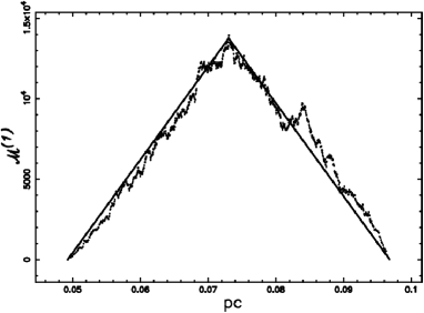
Fig. 18 : Values of concentration computed with equation (89) (full line) compared with the results of a Monte Carlo simulation (filled circles). The parameters in the Monte Carlo 1D random walk are $H_{5}$ = 0.5, $\lambda_{1}$ = 6, $r_{H}=1.6510^{-6}$ pc and NTRIALS = 100.

The theoretical intensity can therefore be evaluated by a numerical integration of equations (88) and (89) along the line of sight, see Fig. 19 and Table 4.

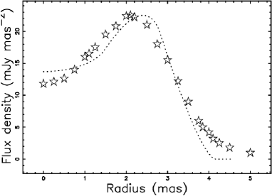
Fig. 19 : Cross-section through the mathematical intensity ${\it I}$ of 1D diffusion in the optically thin case (dashed line, $\chi^{2}=80.64$) and real data (empty stars). Parameters as in Table 4.

Table 4 : Simulation of SN 1993J based on 1D diffusion, optically thin case.

$\displaystyle\hskip 0.0pt{\begin{array}[]{llc}\hline\cr\hline\cr\vskip 6.0pt\cr symbol&meaning&value\\ \vskip 6.0pt\cr\hline\cr\vskip 6.0pt\cr a&radius~{}internal~{}sphere&1.44(mas)\\ \vskip 6.0pt\cr b&radius~{}of~{}shock&2.79(mas)\\ \vskip 6.0pt\cr c&radius~{}external~{}sphere&4.15(mas)\\ \vskip 6.0pt\cr\frac{I_{limb}}{I_{center}}&ratio~{}observed~{}intensities&1.7926\\ \vskip 6.0pt\cr\frac{I_{max}}{I(y=0)}&ratio~{}optically~{}thin&1.6430\\ \vskip 6.0pt\cr\hline\cr\hline\cr\end{array}}$

6.6 Evolution of flux densities

The source of synchrotron luminosity is assumed here to be the flux of kinetic energy, $L_{m}$,

$$L_{m}=\frac{1}{2}\rho 4\pi R^{2}V^{3}\quad,$$ (94)

where $R$ is the instantaneous radius of the SNR and $\rho$ is the density in the advancing layer in which synchrotron emission takes place. The density in the advancing layer is assumed to scale as $R^{-d}$, see formula (8), which means that

$$L_{m}\propto R^{2-d}V^{3}\quad.$$ (95)

The temporal and velocity evolutions can be given by the power law dependencies of equations (17) and (21) and therefore

$$L_{m}\propto t^{-\alpha_{p}d+5\alpha_{p}-3}\quad.$$ (96)

The synchrotron luminosity $L_{\lambda}$ and the observed flux $S_{\lambda}$ at a given wavelength $\lambda$ are assumed to be proportional to the mechanical luminosity and therefore

$$S_{\lambda}=S_{0}(\frac{t}{t_{0}})^{-\alpha_{p}d+5\alpha_{p}-3}\quad,$$ (97)

where $S_{0}$ is the flux at $t=t_{0}$. The availability of synchrotron flux at 6 cm, see Table 1 and Fig. 14 in Marcaide et al. (2009), allows of fixing the parameters $S_{0}$. Fig. 20 reports the observed flux as a function of time as well as a theoretical evaluation using equation (97). The astrophysical version of the above equation is

$$S_{\lambda=6cm}=69.41\,{(\frac{t}{t_{0}}})^{-1.16}~{}mJy\quad,$$ (98)

with the time expressed in years.

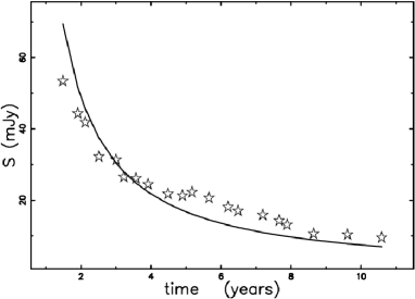
Fig. 20 : Observed time evolution of total flux densities of SN 1993J as given by VLBI data (empty stars) at 6 cm and theoretical relationship as given by formula (97) (full line), with $d$ = 2.79 and $\alpha_{p}=0.82$. The VLBI data at 6 cm are extracted from Table 1 in Marcaide et al. 2009.

7 Conclusions

Law of motion The first two parts of the law of motion for SNR are thought to be a free expansion in which $R\propto t$ and an energy conserving phase in which $R\propto t^{2/5}$. A careful analysis of SN 1993J in the first 10 $yr$ conversely suggest that $R\propto t^{0.82}$. In other words the free expansion which follows the first Newton’s law of motion does not corresponds to the observations. This observational evidence requires a law of motion which contains an adjustable parameter. Here we have chosen as a physical arguments the thin layer approximation in a medium which has a decreasing density of the type $\propto R^{-d}$ The two laws of motion here deduced are the classical nonlinear equation (13) and the complex relativistic-mechanics equation (28). In the classical case of the thin layer approximation, we derived a useful asymptotic law of the type $R\propto t^{1/(4-d)}$, see equation 14. This means that $d=1-1/(\alpha)$ and therefore the value of the $d$ can be deduced from the observational parameter $\alpha$. Both the classical and relativistic equations of the thin layer approximation can be used as a fitting function to deduce the remaining physical parameters , which are the initial radius and the initial velocity or $\beta$.

A third law of motion is deduced in the framework of the relativistic-hydrodynamics with pressure applying the momentum conservation, see equation (37). The two relativistic cases here considered does not have an asymptotic solution. The evaluation of the merit function $\chi^{2}$ , see equation (16) as well the efficiency of the final radius, see equation (6) allows to eliminate the free expansion + the Sedov phase which are supposed to characterize the first two phases of the SNR’s. The best results are obtained by the ”ad hoc” piecewise function (22) followed by the classical nonlinear equation (13) once the $\chi^{2}$ and efficiency are considered together.

Relativistic velocities It is really necessary the relativistic treatment for the equation of motion? We briefly recall that at the moment of writing the maximum observed velocity from CaII H&K absorptions in SN 2002bo  is $\approx 26000km/s$ as measured at -15 days from B maximum , see Figure 11 in Benetti et al. (2004). A shift of 7 days characterizes the time delay between Gamma-ray burst (GRB) and SN spectrum in the case of SN 2003dh  , see Matheson et al. (2003). A quadratic fit allows to extrapolate at t=-22 days from B maximum the velocity of expansion ; in particular we found $\approx 28710km/s$ as a maximum velocity for SN 2002bo  , see data in Figure 11b of Benetti et al. (2004). This means that $\beta\approx 1/10.4$ which is not far from the canonical $\beta=1/10$ which marks the transition from classical to relativistic regime.

Formation of the image The radial decrease in the density of the relativistic electrons from the position of the shock at 3 cm can be obtained by assuming a diffusive process and the resulting intensity of synchrotron emission can be calculated as the integral along the line of sight. Here, we considered the intensity profiles which arise from a 3D mathematical diffusion with constant diffusion coefficient in the optically thin case, see Fig. 13. In this process the particles can be accelerated by the Fermi I mechanism at the shock position in a region of thickness $\ll\,(c-b)\,and\,(b-a)$. In this case the theoretical profile as given in Fig. 13 toward the external region is concave up. A second model with diffusion in 1D with a step length corresponding to the relativistic electron gyro-radius is also analyzed, see the concentration profile given in Fig. 18 and the intensity profile given in Fig. 19. These diffusive processes allow to build up a theoretical 2D map of the shell-like intensity , see Fig. 14. A third model analyzes the radiation from a shell with constant density of emission, see Figure 17. This is the simplest model which produces an ”U” profile in the cut of the intensity which toward the external region is concave down. In this case the accelerating mechanism can be the Fermi II mechanism characterized by multiple collisions in a shell having thickness $b-a$.

A model based on the conversion into radiation of the flux of kinetic energy explains the observed decrease in flux at $6\,cm$, see equation 98 and Figure 20 . This means that a direct conversion of the flux of kinetic energy which varies with time is a realistic model. Due to the fact that the observed profile in intensity is concave up , see Figure 13 , a direct acceleration through the Fermi I mechanism in thin region around the shock is an acceptable model.

References

- Bell (1978) Bell, A.R.: MNRAS 182, 147 (1978)
- Bell (1978) Bell, A.R.: MNRAS 182, 443 (1978)
- Benetti et al. (2004) Benetti, S., Meikle, P., Stehle, M., Altavilla, G., Desidera, S., Folatelli, G.: MNRAS 348, 261 (2004)
- Berg (1993) Berg, H.C.: Random walks in biology. Princeton University Press, Princeton (1993)
- Bevington, P. R. and Robinson, D. K. (2003) Bevington, P. R. and Robinson, D. K.: Data reduction and error analysis for the physical sciences. McGraw-Hill, New York (2003)
- Bohm, Burhop, and Massey (1949) Bohm, D., Burhop, E., Massey, H.: in characteristic of electrical discharges in magnetic fields. McGraw-Hill, New-York (1949)
- Chevalier (1982) Chevalier, R.A.: ApJ 258, 790 (1982)
- Chevalier (1982) Chevalier, R.A.: ApJ 259, 302 (1982)
- Crank (1979) Crank, J.: Mathematics of diffusion. Oxford University Press, Oxford (1979)
- Dermer and Menon (2009) Dermer, C.D., Menon, G.: High Energy Radiation from Black Holes: Gamma Rays, Cosmic Rays, and Neutrinos. Princeton Univerisity Press, Princeton (2009)
- Dyson, J. E. and Williams, D. A. (1997) Dyson, J. E. and Williams, D. A.: The physics of the interstellar medium. Institute of Physics Publishing, Bristol (1997)
- Einstein (1905) Einstein, A.: Annalen der Physik 322, 891 (1905)
- Evans, Hastings, and Peacock (2000) Evans, M., Hastings, N., Peacock, B.: Statistical distributions - third edition. John Wiley & Sons Inc, New York (2000)
- Fermi (1949) Fermi, E.: Physical Review 75, 1169 (1949)
- Fermi (1954) Fermi, E.: ApJ 119, 1 (1954)
- Fransson et al. (2005) Fransson, C., Challis, P.M., Chevalier, R.A., Filippenko, A.V., Kirshner, R.P.: ApJ 622, 991 (2005)
- Freedman et al. (1994) Freedman, W.L., Hughes, S.M., Madore, B.F., Mould, J.R., Lee, M.G.: ApJ 427, 628 (1994)
- French, A.P. (1968) French, A.P.: Special Relativity. CRC, New York (1968)
- Gourgoulhon (2006) Gourgoulhon, E.: EAS PUBL.SER. 21, 43 (2006)
- Hidalgo and Mendoza (2005) Hidalgo, J.C., Mendoza, S.: Physics of Fluids 17, 6101 (2005)
- Hjellming, R. M. (1988) Hjellming, R. M.: Radio stars IN Galactic and Extragalactic Radio Astronomy . Springer, New York (1988)
- Kulsrud (2005) Kulsrud, R.M.: Plasma physics for astrophysics. Princeton University Press, Princeton, N.J. (2005)
- Landau (1987) Landau, L.: Fluid mechanics 2nd edition. Pergamon Press, New York (1987)
- Lang (1999) Lang, K.R.: Astrophysical formulae. (Third Edition). Springer, New York (1999)
- Longair (1994) Longair, M.S.: High energy astrophysics. Cambridge University Press, 2nd ed., Cambridge (1994)
- Marcaide et al. (2009) Marcaide, J.M., Martí-Vidal, I., Alberdi, A., Pérez-Torres, M.A.: A&A 505, 927 (2009)
- Marti-Vidal et al. (2010) Marti-Vidal, I., Marcaide, J.M., Alberdi, A., Guirado, J.C., Perez-Torres, M.A., Ros, E.: ArXiv : 1007.1224 (2010)
- Matheson et al. (2003) Matheson, T., Garnavich, P.M., Stanek, K.Z., Bersier, D.: ApJ 599, 394 (2003)
- McCray and Layzer (1987) McCray, A. R. In: Dalgarno, Layzer, D. (eds.): Spectroscopy of astrophysical plasmas. Cambridge University Press, Cambridge (1987)
- Oort (1946) Oort, J.H.: MNRAS 106, 159 (1946)
- Padmanabhan (2001) Padmanabhan, P.: Theoretical astrophysics. Vol. II: Stars and Stellar Systems. Cambridge University Press, Cambridge, MA (2001)
- Press et al. (1992) Press, W.H., Teukolsky, S.A., Vetterling, W.T., Flannery, B.P.: Numerical recipes in FORTRAN. The art of scientific computing. Cambridge University Press, Cambridge (1992)
- Ripero et al. (1993) Ripero, J., Garcia, F., Rodriguez, D., Pujol, P., Filippenko, A.V., Treffers, R.R., Paik, Y., Davis, M., Schlegel, D., Hartwick, F.D.A., Balam, D.D., Zurek, D., Robb, R.M., Garnavich, P., Hong, B.A.: IAU circ. 5731, 1 (1993)
- Rybicki and Lightman (1991) Rybicki, G., Lightman, A.: Radiative processes in astrophysics. Wiley-Interscience, New-York (1991)
- Sedov (1959) Sedov, L.I.: Similarity and Dimensional Methods in Mechanics. Academic Press, New York (1959)
- Somov (2006) Somov, B.V.: Plasma Astrophysics, Part I: Fundamentals and Practice. Springer, New-York (2006)
- Truelove and McKee (1999) Truelove, J.K., McKee, C.F.: ApJS 120, 299 (1999)
- Weinberg (1972) Weinberg, S.: Gravitation and Cosmology: Principles and Applications of the General Theory of Relativity. John Wiley & Sons, Inc., New York (1972)
- Zaninetti (2007) Zaninetti, L.: Baltic Astronomy 16, 251 (2007)
- Zaninetti (2009) Zaninetti, L.: MNRAS 395, 667 (2009)
- Zaninetti and Siah (1988) Zaninetti, L., Siah, M.J.: A&A 201, 21 (1988)