Rationality in the Theory of the Firm

Abstract

We have previously presented a critique of the standard Marshallian theory of the firm, and developed an alternative formulation that better agreed with the results of simulation. An incorrect mathematical fact was used in our previous presentation. This paper deals with correcting the derivation of the Keen equilibrium, and generalising the result to the asymmetric case. As well, we discuss the notion of rationality employed, and how this plays out in a two player version of the game.

1 Introduction

Keen [3, Ch 4] pointed out a fundamental flaw with the standard Marshallian theory of the firm, whereby the market demand function $P(Q)$ (price of a good given total market production Q) is assumed to be a decreasing function of $Q$ (i.e. $P^{\prime}(Q)<0$), yet at the same time, for a large number of firms, each individual firm’s production $q_{i}$ has no effect on market price, ie $\partial P/\partial q_{i}=0$. Yet it is easy to see from elementary calculus, that these two conditions cannot be true simultaneously, as first noted by Stigler [7].

Marshallian analysis proceeds under this assumption that individual firms’ actions have no effect on the market, leading to the profit maximum for each firm to occur when it’s marginal cost is equal to the market price.

In [5, 4], we argue that the economy’s equilibrium will not occur at the zero of the partial derivative of the individual profit function, but rather when the total derivative of each individual profit with respect to market production is simultaneously satisfied. This leads to a revised prediction of the difference between market price and marginal cost being related to the slope of the demand curve:

$$P(Q)-MC(q_{i})=-nq_{i}P^{\prime}(Q)$$ (1)

Furthermore, a simple reactive rational agent model of the firm produced results compatible with the Keen equilibrium, and not the Cournot-Nash equilibrium predicted from standard Marshallian analysis. It should be pointed out that this agent model makes neither the partial derivative assumption of Marshallian analysis, nor the total derivative assumption of Keen’s analysis, but rather the agents seek to always optimise their profits assuming the past is a guide to the future.

Anglin [2] critiqued our 2006 paper, but the critique was not without its own mathematical difficulties. We extensively rebutted his paper in a submission to the same journal in which our 2006 paper, and Anglin’s critique appeared. This was rejected on editorial privilege. We chose not to publish the rebuttal in another journal, as the rebuttal doesn’t advance the state of the field, but have made it available via arXiv [6], for thos who might be interested.

Nevertheless, in the course of corresponding with Anglin, the main issue bothering Anglin was identified as an erroneous mathematical assumption we made for the value of $dq_{i}/dQ$, for which no such assumption can be made. This paper serves to correct the analysis, and also correctly generalise the Keen analysis to the asymmetric firm case. As a consequence, our previous attempt described in section 3 of [4], which Anglin ridiculed as “conjectural variation”, is no longer relevant.

The purpose of this paper is not to rebut Anglin’s paper, but to correct a problematic assertion in our work, and consequently extend the Keen analysis to asymmetric firm response.

2 The profit formula

We take as our starting point, the usual profit formula of a single product market with $n$ firms:

$$\pi_{i}=q_{i}P(Q)-\int_{0}^{q_{i}}MC(q_{i})dq_{i},$$ (2)

where $\pi_{i}$ is the profit obtained by firm $i$, as a function of its production $q_{i}$, and the total market production $Q=\sum_{i}q_{i}$. The function $P(Q)$ is the demand curve, namely the price the good achieves when $Q$ items of the good is available on the market. In the following, $P(Q)$ is taken to be a monotonically decreasing curve ($P^{\prime}<0$). The function $MC(q_{i})$ is the marginal cost of producing an extra item of the good, given that a firm is producing $q_{i}$ items.

3 Rationality

The key concept of the rational agent, or homo economicus is that the agent chooses from an array of actions so as to maximise some utility function. In the context of the theory of the firm, the utility functions are given by $\pi_{i}$ in eq (2), and the choices are the production values chosen by the individual firms.

Intrinsic to the notion of rationality is the property of determinism. Given a single best course of action that maximises utility, the agent must choose that action. Only where two equally good courses of action occur, might the agents behave stochastically. This deterministic behaviour of the agents is the key to understanding the stability of the Keen equilibrium, and the instability of the Cournot equilibrium, which is the outcome of traditional Marshallian analysis.

When setting up a game, it is important to circumscribe what information the agents have access to. Clearly, if the agents know what the total market production $Q$ will be in the next cycle, as well as their marginal cost $MC$, the rational value of $q_{i}$ can be found by setting the partial derivative of $\pi_{i}$ to zero:

$$\frac{\partial\pi_{i}}{\partial q_{i}}=P+q_{i}\frac{\partial P}{\partial q_{i}}-MC(q_{i})=0.$$ (3)

Indeed, the Marshallian theory further assumes that in the limit as the number of firms $n$ tends to infinity, the term $\partial P/\partial q_{i}\rightarrow 0$, to arrive at the ultimate result that price will tend to the marginal cost (assuming a unique marginal cost exists over all firms)[1, p. 322]. This assumption is strictly false, as shown by [7]. Instead, $\partial P/\partial q_{i}=dP/dQ$, which is independent of the number firms in the economy. The Cournot-Nash model starts with each agent knowing that all other agents are rational, and their marginal cost curves, consequently (under the right circumstances) being able to predict the optimal production levels for each agent. Therefore, the total production $Q$ is predictable, and equation (3) should hold. Furthermore, for certain distributions of market share (eg the symmetric case of equal market share where $q_{i}=Q/n$), individual production levels vanish in the limit $n\rightarrow\infty$. Therefore $P\rightarrow MC$. This result is known as the Cournot theorem.

However, it is completely unrealistic for the firms to be able to predict market production (and hence price). Firms cannot know whether their competitors will act completely rationally, and details such as the marginal cost curve for each firm, and even the total number of players is unlikely to be known. So equation (3) cannot be correct. Instead, firms can really only assume that the price tomorrow will most likely be similar today, and that the best they can do is incrementally adjust their output to “grope for” the optimal production value. So in our model, firms have a choice between increasing production or decreasing it. If the previous round’s production change caused a rise in profits, the rational thing to do is to repeat the action. If, on the other hand, it leads to a decrease in profit, the opposite action should be taken. At equilibrium, one would expect the production to be continuously increased and decreased in a cycle with no net movement.

4 Game theoretic analysis of the Cournot equilibrium

For simplicity, assume a two firm system with identical constant marginal costs, that has been initialised at its Cournot equilibrium ($P+QP^{\prime}/2-MC=0,q_{1}=q_{2}=Q/2$). There are three possible outcomes for the next step:

1. Both firms increase production. This reduces the price fetched for each firm. The right hand side of equation 3 becomes negative, reducing the profits of both firms. The logical next step is for both firms to decrease production, which is covered under item 3

2. One firm increases production whilst the other decreases it. If the production increment is the same in each case, then the market price does not change. The net effect is of one firm gaining market share at the expense of the other. In this case, the firm losing market share will switch to increasing production, whilst the other firm will continue increasing production. This is situation described by item 1.

   If the production increments differed between firms, then there are two cases: if the firm with larger increment increases, and the increment is sufficiently big, then profit levels will fall for both firms. The dynamics returns to the original (Cournot) point. Otherwise, the firm losing market share will switch to increasing, which is situation 1.

3. Both firms decrease production. In this case, provided the price is higher than the monopoly price, both firms’ profits will rise, leading to another round of production decreases.

The net result is that the Cournot equilibrium is unstable in the direction of both firms decreasing production. The n-firm case can be analysed in the same way [5]. The situation where the majority of firms are decreasing their production simultaneously will occur by chance within a few cycles of the system initialisation. From there, the entrainment of all firms into the production-reducing behaviour happens rapidly, until the system stabilises at monopoly prices.

It is important to note, that this effect depends on the deterministic nature of the agent behaviour, a result of the assumption of rationality. Presumably, most real economic agents are not as rational as this, and the introduction of 30% irrationality into the agents is sufficient to ensure competitive pricing [5].

5 Derivation of the Keen equilibrium

Mathematically, global equilibrium will occur when all partial derivatives $\partial\pi_{i}/\partial q_{j}$ vanish. However, this situation can never pertain, as $\forall i\neq j,\,\partial\pi_{i}/\partial q_{j}=q_{i}P^{\prime}<0$, except possibly for the trivial solution $Q=0$.

Instead we propose the condition that all firm’s profits are maximised with respect to total industry output $d\pi_{i}/dQ=0$. This constrains the dynamics of firms’ outputs to an $n-1$-dimensional polyhedron, but otherwise does not specify what the individual firms should do. As an equilibrium condition, it is vulnerable to a single firm “stealing” market share. However, no firm acts in isolation. The other firms will react, negating the benefit obtained by first firm, causing the system to settle back to the $d\pi_{i}/dQ=0$ manifold.

The derivation of the Keen equilibrium follows the presentation in [4]. The total derivative of an individual firm’s profit is given by

$$\frac{d\pi_{i}}{dQ}=P\frac{dq_{i}}{dQ}+q_{i}\frac{dP}{dQ}-MC(q_{i})\frac{dq_{i}}{dQ}$$ (4)

which is zero at the Keen equilibrium.

In terms of the model introduced in §4, there is no absolute equilibrium, but rather a limit cycle where the individual firms are “jiggling” their outputs around the equilibrium value. If we average over this limit cycle, and retaining only zeroth order terms in $\Delta q_{i}$, we get

$$\left\langle\frac{d\pi_{i}}{dQ}\right\rangle = P(\langle Q\rangle)\left\langle\frac{dq_{i}}{dQ}\right\rangle+\langle q_{i}\rangle P^{\prime}(\langle Q\rangle)-MC(\langle q_{i}\rangle)\left\langle\frac{dq_{i}}{dQ}\right\rangle$$ (5)

$$= P\theta_{i}+q_{i}P^{\prime}-MC(q_{i})\theta_{i}=0.$$

where $\theta_{i}=\langle dq_{i}/dQ\rangle$ and the terms $P$, $P^{\prime}$ and $q_{i}$ refer to the equilibrium average values of these quantities. The $\theta_{i}$ terms are normalised: $\sum_{i}\theta_{i}=dQ/dQ=1$. They can be considered to be the (normalised) responsiveness of the firms to changing market conditions

The symmetric firm case corresponds to setting $\theta_{i}=1/n$, which leads to the equation:

$$P+nq_{i}P^{\prime}-MC(q_{i})=0$$ (6)

which is equation (6) of [4].

In our previous expositions [4, 5], we incorrectly set $dq_{i}/dQ=\sum_{j}\partial q_{j}/\partial q_{i}=1$, which as pointed out in a critique by Paul Anglin[2], when coupled with $q_{i}(Q=0)=0$ leads to the unjustifiable conclusion that $q_{i}=Q/n$ at all times. Now, in equation (5), the values $\theta_{i}$ only refer to the derivatives at equilibrium, so there is no necessity for (6) to entail an equi-partition of the market share.

6 Testing the Keen equilibrium

We can use an agent-based computational model based on the model introduced in §4 to test the Keen equilibrium, or more specifically, equation (5). The terms $P(Q)$, $q_{i}$ and $MC_{i}$ are all available as part of the model. In addition, each agent has an attribute $\delta_{i}$, which is the amount that agent $i$ varies its production up or down each time step.

We can compute the quantity $\theta_{i}$ by averaging $\Delta q_{i}/\Delta Q$ over $\theta_{w}=10$ time steps.

In the following experiment with 1000 firms, we used a linear pricing function $P=11-Q/3$, and constant marginal costs $MC_{i}$ drawn uniformly from the range $[0.5,0.5)$. The $\delta_{i}$ increments were drawn from a half normal distribution — ie the absolute values of normally distributed deviates with zero mean and standard deviation $0.002/n$. The code implementing the model, and the experimental parameter script is available as firmmodel.1.D7, from the EcoLab website (http://ecolab.sf.net).

Figure 1 shows the histogram of values taken by the statistic $q_{i}P^{\prime}+\theta_{i}(P-M_{i})$ for the 1000 firms over 1378 replications. The vast majority of observed values are consistent with zero, the predicted value of eq (5), however there is a significant minority of outliers, which are not explained within the theory presented in §5.

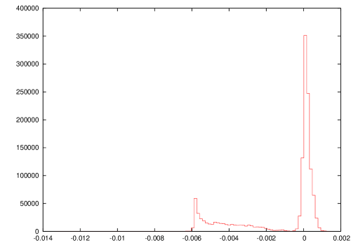
Figure 1: Histogram of the statistic $q_{i}P^{\prime}+\theta_{i}(P-MC_{i})$ for 1378 replications of the 1000 firm model. Most of the values are clustered close to zero, but a sizable minority have non-zero negative values. The left hand half of the histogram also has non-zero bins, but are not visible with the shown vertical scale

We can, however, consider the statistic $\xi=q_{i}P^{\prime}/(M_{i}-P)$, which in the Cournot theory should be one by (3). Figure 2 shows a histogram of $\xi$ for a single run of the 1000 firm model. The values approximately fit a lognormal distribution, from which we can see that value $\xi=1$ lies some 35 “sigmas” to the right of the mean, ie the Cournot prediction (3) is excluded to the tune of $p\approx 10^{-267}$.

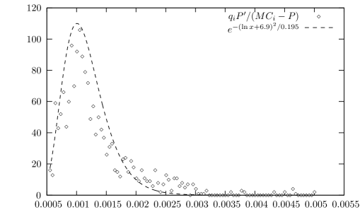
Figure 2: Histogram of the statistic $q_{i}P^{\prime}/(MC_{i}-P)$ for a single run of the 1000 firm model. The dashed line shows a fitted log-normal distribution.

7 Conclusion

In this paper, we have discussed the behaviour of an n-player game of rational, but not clairvoyant, agents. This exhibits a phase of coordinated behaviour of the agents that brings market prices to near monopoly levels due to the very rationality of the agents rather than any overt coordination mechanism. We use numerical simulations to reject the traditional Cournot-Nash solution of the game.

References

- [1] J.R.Green A. Mas-Colell, M.D. Whinston. Microeconomics. Oxford University Press, New York, 1995.
- [2] Paul Anglin. On the proper behavior of atoms: A comment on a critique. Physica A, 387:277–280, 2008.
- [3] Stephen Leslie Keen. Debunking Economics: The Naked Emperor of the Social Sciences. Zed Books, 2002.
- [4] Steve Keen and Russell Standish. Profit maximisation, industry structure, and competition: a critique of neoclassical theory. Physica A, 370:81–85, 2006.
- [5] Russell Standish and Steve Keen. Emergent effective collusion in an economy of perfectly rational competitors. In Proceedings 7th Asia-Pacific Conference on Complex Systems, page 228, Cairns, December 2004. nlin.AO/0411006.
- [6] Russell Kim Standish and Stephen Leslie Keen. Comment on “on the proper behavior of atoms” by paul anglin. arXiv:1309.3369, 2010.
- [7] George J. Stigler. Perfect competition, historically contemplated. The Journal of Political Economy, 65:1–17, 1957.