Quotient cohomology for tiling spaces

Abstract.

We define a relative version of tiling cohomology for the purpose of comparing the topology of tiling dynamical systems when one is a factor of the other. We illustrate this with examples, and outline a method for computing the cohomology of tiling spaces of finite type.

1. Introduction

Since its development, cohomology has been an essential tool of algebraic topology. It is a topological invariant that can tell spaces apart (both with the groups and with the ring structure). It is computable by a variety of cut-and-paste rules. It is a functor that relates two or more spaces and the maps between them. Finally, it is the setting for other topological structures, such as characteristic classes.

The cohomology of tiling spaces is far less developed, and in some ways resembles the state of abstract cohomology in the mid-20th century. Mostly it has been used to tell spaces apart. There has been little progress in using cut-and-paste arguments to compute anything, and most computations have relied on inverse limit structures. It is only used to study one space at a time, not in a functorial setting. We have a limited understanding of what cohomology tells us, and what other problems can be addressed using cohomology. (However, see [B, BBG, CGU, CS, S1] for some applications to gap labeling, deformations, spaces of measures, and exact regularity.)

This paper is an attempt to remedy this deficiency. By specializing the algebraic mapping cylinder and mapping cone construction to tiling theory, we develop a relative version of tiling cohomology, which we call quotient cohomology. We then show how to use quotient cohomology to relate similar tiling spaces.

In Section 2, we lay out the definitions and basic properties of quotient cohomology. In Section 3 we illustrate the formalism with some simple examples, both from basic topology and from one dimensional tilings. In Section 4 we develop the tools needed to handle more complicated problems. The key tool for tiling theory is Proposition 4, which describes how to get the quotient cohomology of two tiling spaces that differ only on the suspension of a lower-dimensional tiling space. In Section 5 we examine a family of nine tiling spaces that includes the 2-dimensional dyadic solenoid and the “chair” substitution tiling. By applying Proposition 4 repeatedly, we relate the cohomology of each space to that of the dyadic solenoid. Finally, in Section 6 we explore the cohomology of tiling spaces of finite type, a class of tiling spaces that has previously defied analysis.

2. Definitions

A tiling of $\mathbb{R}^{d}$ is a collection of closed topological disks, called tiles, such that tiles overlap only on their boundaries and such that the union of all the tiles is $\mathbb{R}^{d}$. In addition to their position and geometric shape, tiles may carry labels. The translation group $\mathbb{R}^{d}$ transforms a tiling into a different tiling by moving all tiles simultaneously. If $\mathcal{T}$ is a tiling, then $\mathcal{T}-v$ is the tiling translated by $v\in\mathbb{R}^{d}$. We endow the orbit of $\mathcal{T}$ under translation with a metric where two tilings are $\epsilon$-close if they agree, up to a translation by $\epsilon$ or less, on a ball of radius $\epsilon^{-1}$ around the orgin. The completion $X_{\mathcal{T}}$ of the orbit of $\mathcal{T}$ is called the hull of $\mathcal{T}$, or the tiling space associated with $\mathcal{T}$. Locally, $X_{\mathcal{T}}$ is the product of $\mathbb{R}^{d}$ with a totally disconnected space, typically a Cantor set. $X_{\mathcal{T}}$, equipped with the action of the translation group $\mathbb{R}^{d}$, is a tiling dynamical system. Most of the tiling dynamical systems in the literature are compact, minimal and uniquely ergodic.

Substitutions provide an important method for the generation of tilings. A $d$-dimensional substitution is a recipe that linearly inflates each of a finite collection of $d$-dimensional prototiles and specifies a tiling of each of the inflated prototiles by translates of the prototiles. A tiling of $\mathbb{R}^{d}$ obtained as a limit of repeated application of a substitution is called a substitution tiling and its hull is a substitution tiling space. Under mild assumptions ([So]), a substitution induces a substitution homeomorphism on its tiling space.

Besides their intrinsic interest, tiling dynamical systems model a variety of structures in dynamics; for instance, every 1-dimensional orientable expanding attractor is topologically conjugate to either the shift homeomorphism on a solenoid or the substitution homeomorphism on a substitution tiling space [AP]. For background information on tiling spaces and their topology, see [S3].

If $X$ and $Y$ are topological spaces and $f:X\to Y$ is an injection, then the relative (co)homology groups $H_{k}(Y,X)$ and $H^{k}(Y,X)$ relate the (co)homology of $X$ and $Y$ via long exact sequences

$$\cdots\to H_{k+1}(Y,X)\to H_{k}(X)\xrightarrow{f_{*}}H_{k}(Y)\to H_{k}(Y,X)\to\cdots,$$

$$\cdots\to H^{k}(Y,X)\to H^{k}(Y)\xrightarrow{f^{*}}H^{k}(X)\to H^{k+1}(Y,X)\to\cdots.$$

Factor maps between minimal dynamical systems are surjections, since the image of each orbit is dense, but typically are not injections. To study such spaces, we need a different tool.

Let $f:X\to Y$ be a quotient map such that the pullback $f^{*}$ is injective on cochains. This is the typical situation for covering spaces, for branched covers, and for factor maps between tiling spaces. When dealing with tiling spaces, “cochains” can either mean Čech cochains or pattern-equivariant cochains [K, KP, S2]; our arguments apply equally well to both. Define the cochain group $C_{Q}^{k}(X,Y)$ to be $C^{k}(X)/f^{*}(C^{k}(Y))$. The usual coboundary operator sends $C_{Q}^{k}(X,Y)$ to $C_{Q}^{k+1}(X,Y)$, and we define the quotient cohomology $H_{Q}^{k}(X,Y)$ to be the kernel of the coboundary modulo the image. By the snake lemma, the short exact sequence of cochain complexes

$$0\to C^{k}(Y)\xrightarrow{f^{*}}C^{k}(X)\to C_{Q}^{k}(X,Y)\to 0$$

induces a long exact sequence

$$\cdots\to H^{k-1}_{Q}(X,Y)\to H^{k}(Y)\xrightarrow{f^{*}}H^{k}(X)\to H^{k}_{Q}(X,Y)\to\cdots$$ (1)

relating the cohomologies of $X$ and $Y$ to $H_{Q}^{*}(X,Y)$.

Quotient cohomology is related to an ordinary relative cohomology group involving the mapping cylinder $M_{f}=(X\times[0,1])\coprod Y/\sim$, where $(x,1)\sim f(x)$, or to the reduced cohomology of a mapping cone, where we collapse $X\times\{0\}\subset M_{f}$ to a single point. $M_{f}$ is homotopy equivalent to $Y$, and the inclusion $i:X\to M_{f}$, $i(x)=(x,0)$ is homotopically the same as $f$. This yields the (standard) long exact sequence in relative cohomology

$$\cdots H^{k}(M_{f},X)\to H^{k}(M_{f})\xrightarrow{i^{*}}H^{k}(X)\to H^{k+1}(M_{f},X)\to\cdots.$$ (2)

Applying the Five Lemma to the long exact sequences (1) and (2) and noting that $H^{k}(M_{f})\simeq H^{k}(Y)$, with $i^{*}$ essentially the same as $f^{*}$, we see that $H_{Q}^{k}(X,Y)$ equals $H^{k+1}(M_{f},X)$.

Quotient cohomology can also be viewed as the cohomology of the algebraic mapping cone of $X$ and $Y$ [W]. Specifically, let $C^{k}_{f}=C^{k}(X)\oplus C^{k+1}(Y)$, and let $d_{f}(a,b)=(d_{X}(a)+f^{*}(b),-d_{Y}(b))$. The cohomology of $d_{f}$ fits into the same exact sequence as $H^{k}_{Q}(X,Y)$, and hence is isomorphic to $H^{k}_{Q}(X,Y)$. Indeed, the mapping cone construction works even when $f^{*}$ is not injective at the level of cochains.

The mapping cylinder and cone constructions are extremely general. They are also cumbersome, and to the best of our knowledge have never been used in tiling theory. Indeed, many of the structures defined for tiling spaces, such as pattern-equivariant cohomology [K, KP], rely on an identification of certain features of a tiling $\mathcal{T}$ with sets of tilings in $X_{\mathcal{T}}$. These structures make no sense on a (topological) mapping cylinder. Fortunately, quotient cohomology does make sense, and provides an easy yet powerful tool for studying the topology of tiling spaces.

3. Topological and tiling examples

3.1. Basic topological examples

Example 1.

Let $Y$ be a CW complex with a distinguished $n$-cell $e^{n}$ that is not on the boundary of any cell of higher dimension. Let $X$ be the same complex, only with two copies of $e^{n}$ (call them $e^{n}_{1}$ and $e^{n}_{2}$), each with the same boundary as $e^{n}$, and let $f$ be the map that identifies $e^{n}_{1}$ and $e^{n}_{2}$. Then, working with cellular cohomology, $C_{Q}^{k}(X,Y)$ is trivial in all dimensions except $k=n$, and $C_{Q}^{n}(X,Y)$ is generated by the duals $(e^{n}_{i})^{\prime}$ to $e^{n}_{i}$, with the relation $(e^{n}_{1})^{\prime}+(e^{n}_{2})^{\prime}=0$, so $H_{Q}^{k}(X,Y)=\mathbb{Z}$ if $k=n$ and is zero otherwise.

Slightly more generally, let $X$ be a CW complex and let $Y$ be the quotient of $Y$ by the identification of two $n$-cells $e^{n}_{1,2}$ of $X$, whose boundaries have previously been identified. (The generalization is that we make no assumptions about how higher-dimensional cells attach to $e^{n}_{1,2}$.) Then, as before, $C_{Q}^{k}(X,Y)=\mathbb{Z}$ when $k=n$ and vanishes otherwise, so $H_{Q}^{k}(X,Y)=\mathbb{Z}$ for $k=n$ and vanishes otherwise. Up to homotopy, identifying $e^{n}_{1,2}$ is the same thing as gluing in an $(n+1)$-cell with boundary $e^{n}_{1}-e^{n}_{2}$, in which case $f$ can be viewed as an inclusion into a space $Y^{\prime}$ that is homotopy equivalent to $Y$, and $H^{k}_{Q}(X,Y)=H^{k+1}(Y^{\prime},X)$.

Repeating the construction as needed, we can compute the quotient cohomology of any two CW complexes $X$ and $Y$, where $Y$ is the quotient of $X$ by identification of some cells.

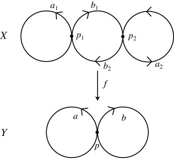
Figure 1. A simple example of quotient cohomology.

Example 2.

Figure 1 shows two graphs, with $X$ the double cover of $Y$. Let $f$ be the covering map, sending each edge $a_{i}$ to $a$, each $b_{i}$ to $b$, and each vertex $p_{i}$ to $p$. Since $f^{*}(p^{\prime})=p_{1}^{\prime}+p_{2}^{\prime}$, $f^{*}(a^{\prime})=a_{1}^{\prime}+a_{2}^{\prime}$ and $f^{*}(b^{\prime})=b_{1}^{\prime}+b_{2}^{\prime}$, $C_{Q}^{0}(X,Y)=\mathbb{Z}$ is generated by $p_{1}^{\prime}$, with $p_{2}^{\prime}=-p_{1}^{\prime}$, while $C_{Q}^{1}(X,Y)=\mathbb{Z}^{2}$ is generated by $a_{1}^{\prime}$ and $b_{1}^{\prime}$, with $a_{2}^{\prime}=-a_{1}^{\prime}$ and $b_{2}^{\prime}=-b_{1}^{\prime}$. The coboundary of $p_{1}^{\prime}$ is $b_{2}^{\prime}-b_{1}^{\prime}=-2b_{1}^{\prime}$, so $H_{Q}^{0}(X,Y)=0$ and $H_{Q}^{1}(X,Y)=\mathbb{Z}\oplus\mathbb{Z}_{2}$, with generators $a_{1}^{\prime}$ and $b_{1}^{\prime}$. Our long exact sequence (1) is then

$$0\to\mathbb{Z}\xrightarrow{f^{*}}\mathbb{Z}\to 0\to\mathbb{Z}^{2}\xrightarrow{f^{*}}\mathbb{Z}^{3}\to\mathbb{Z}\oplus\mathbb{Z}_{2}\to 0.$$ (3)

Torsion appears in $H^{1}_{Q}(X,Y)$, reflecting the fact that $f^{*}(b^{\prime})$ is cohomologous to $2b_{1}^{\prime}\in H^{1}(X)$.

3.2. One-dimensional tiling examples

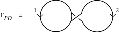
Figure 2. The approximant for the period-doubling substitution tiling

Example 3 (Period Doubling over the 2-Solenoid).

The period doubling substitution is $1\to 21$, $2\to 11$. (By this we mean that there are two prototiles, each of the same length, one labeled 1 and the other 2. The substitution inflates each prototile by a factor of two, tiling the inflated 1 with a 2 and a 1, and the inflated 2 by two 1’s.) Since this is a substitution of constant length 2, there is a natural map from the period doubing tiling space $\Omega_{PD}$ to the dyadic solenoid $S_{2}$. $\Omega_{PD}$ can be written as the inverse limit via substitution of the approximant $\Gamma_{PD}$ shown in Figure 2, where the long edges 1 and 2 represent tile types and the short edges represent possible transitions [BD]. $\Gamma_{PD}$ is homotopically a figure 8, and maps to a circle by identifying the two long edges and identifying the three short edges. This projection of $\Gamma_{PD}$ to the circle intertwines the substitution on $\Gamma_{PD}$ and the doubling map on $S^{1}$, and has quotient cohomology $H^{1}_{Q}(\Gamma_{PD},S^{1})=\mathbb{Z}$ (and $H^{0}_{Q}=0$). The dyadic solenoid $S_{2}$ is the inverse limit of a circle under doubling, and $H^{k}_{Q}(\Omega_{PD},S_{2})$ is the direct limit of $H^{k}_{Q}(\Gamma_{PD},S^{1})$ under substitution. Substitution acts on $H^{1}_{Q}(\Gamma_{PD},S^{1})$ by multiplication by $-1$, so $H^{1}_{Q}(\Omega_{PD},S_{2})=\varinjlim H^{1}_{Q}(\Gamma_{PD},S^{1})=\mathbb{Z}$.

Example 4.

The Thue-Morse substitution tiling of the real line is well known to be the double cover of the period-doubling tiling. Here we explore the quotient cohomology of the pair.

The Thue-Morse substitution is $A\to AB$, $B\to BA$. We can rewrite this in terms of collared tiles, distinguishing between $A$ tiles that are followed by $B$ tiles (call these $A_{1}$) and $A$ tiles that are followed by $A$ tiles (call these $A_{2}$). Likewise, $B$ tiles that are followed by $A$ tiles are called $B_{1}$ and $B$ tiles that are followed by $B$ tiles are $B_{2}$. In terms of these collared tiles, the substitution is:

$$A_{1}\to A_{1}B_{2};\qquad A_{2}\to A_{1}B_{1};\qquad B_{1}\to B_{1}A_{2};\qquad B_{2}\to B_{1}A_{1}.$$ (4)

The map from the Thue-Morse substitution space to the period-doubling space just replaces each $A_{1}$ or $B_{1}$ tile with a 1 and each $A_{2}$ or $B_{2}$ with a 2. This is exactly 2:1, and the preimage of any period-doubling tiling consists of a Thue-Morse tiling, plus a second tiling obtained by swapping $A_{i}\leftrightarrow B_{i}$ at each place.

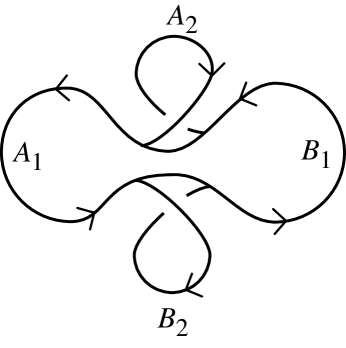
Figure 3. The approximant $\Gamma_{TM}$ for the Thue-Morse substitution tiling space.

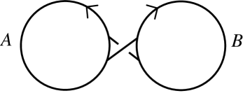
Figure 4. Another approximant $\Gamma_{TM^{\prime}}$ for the Thue-Morse tiling space.

Using collared tiles, we obtain the Thue-Morse tiling space $\Omega_{TM}$ as the inverse limit, under the substitution (4), of the approximant $\Gamma_{TM}$ shown in Figure 3. $\Gamma_{TM}$ is homotopy equivalent to the double cover of a figure 8, just as $\Gamma_{PD}$ is equivalent to a figure 8. Indeed, the quotient map from $\Gamma_{TM}$ to $\Gamma_{PD}$ is, up to homotopy, the covering map of the figure 8 that we studied in Example 2, with $H^{1}_{Q}(\Gamma_{TM},\Gamma_{PD})=\mathbb{Z}\oplus\mathbb{Z}_{2}$, with $A_{1}^{\prime}$ (or $B_{1}^{\prime}$) generating the $\mathbb{Z}_{2}$ factor and $A_{2}^{\prime}$ (or $B_{2}^{\prime}$) generating the $\mathbb{Z}$ factor.

Under substitution, $A_{1}^{\prime}+A_{2}^{\prime}$ pulls back to $A_{1}^{\prime}+B_{1}^{\prime}+A_{2}^{\prime}+B_{2}^{\prime}=0$, while $A_{1}^{\prime}$ pulls back to $A_{1}^{\prime}+A_{2}^{\prime}+B_{2}^{\prime}=A_{1}^{\prime}$, and $H_{Q}^{1}(\Omega_{TM},\Omega_{PD})=\varinjlim H_{Q}^{1}(\Gamma_{TM},\Gamma_{PD})=\mathbb{Z}_{2}$. The groups $H^{1}(\Omega_{TM})$ and $H^{1}(\Omega_{PD})$ are both isomorphic to $\mathbb{Z}[{\textstyle\frac{1}{2}}]\oplus\mathbb{Z}$ and the exact sequence (1) applied to $\Omega_{TM}$ and $\Omega_{PD}$ is

$$0\to\mathbb{Z}\xrightarrow{f^{*}}\mathbb{Z}\to 0\to\mathbb{Z}[{\textstyle\frac{1}{2}}]\oplus\mathbb{Z}\xrightarrow{f^{*}}\mathbb{Z}[{\textstyle\frac{1}{2}}]\oplus\mathbb{Z}\to\mathbb{Z}_{2}\to 0.$$ (5)

Although $H^{1}(\Omega_{TM})$ and $H^{1}(\Omega_{PD})$ are isomorphic as abstract groups, the pullback map $f^{*}$ is not an isomorphism. Rather, it is the identity on $\mathbb{Z}[{\textstyle\frac{1}{2}}]$ and multiplication by 2 on $\mathbb{Z}$.

The remaining one dimensional examples may seem trivial or contrived, but they are the building blocks for understanding the 2-dimensional examples that follow.

Example 5 (Degenerations A and B.).

If $X=S_{2}\times\{1,2\}$ is 2 copies of a dyadic solenoid and $Y=S_{2}$ is a single copy, and if $f$ is projection onto the first factor, then $H^{1}_{Q}(X,Y)=H^{1}(S_{2})=\mathbb{Z}[{\textstyle\frac{1}{2}}]$ and $H^{0}_{Q}(X,Y)=H^{0}(S_{2})=\mathbb{Z}$. We call this degeneration A. Degeneration B is where $X=\Omega_{PD}\times\{1,2\}$ projects to $Y=\Omega_{PD}$, in which case $H^{1}_{Q}(X,Y)=H^{1}(\Omega_{PD})=\mathbb{Z}[{\textstyle\frac{1}{2}}]\oplus\mathbb{Z}$ and $H^{1}_{Q}(X,Y)=H^{0}(\Omega_{PD})=\mathbb{Z}$.

Example 6 (Degeneration C.).

The space $\Gamma_{TM^{\prime}}$ of Figure 4 also serves as an approximant for another tiling space of interest using a different substitution map. Let $X$ be the inverse limit of the $\Gamma_{TM^{\prime}}$ under a map that wraps each large circle twice around itself, and that doubles the length of the small intervals that link the circles. That is, the interval that goes from the left circle to the right one turns into a piece of the left circle followed by the interval, followed by a piece of the right circle. Note that the small loop obtained from the four small intervals is homologically invariant under this map.

Let $Y=S_{2}$ be the dyadic solenoid, viewed as the inverse limit of a circle under doubling. The obvious map from $\Gamma_{TM^{\prime}}$ to $S^{1}$ has $H^{1}_{Q}(\Gamma_{TM^{\prime}},S^{1})=\mathbb{Z}\oplus\mathbb{Z}$ and $H^{0}_{Q}(\Gamma_{TM^{\prime}},S^{1})=0$. Substitution multiplies the first factor in $H^{1}_{Q}$ by 2 and the second factor by 1, so $H^{1}_{Q}(X,Y)=\varinjlim H^{1}_{Q}(\Gamma_{TM^{\prime}},S^{1})=\mathbb{Z}[{\textstyle\frac{1}{2}}]\oplus\mathbb{Z}$, while $H^{0}_{Q}(X,Y)=0$.

4. Tools

Suppose that $f:X\to\ Y$ and $g:Y\to Z$ are quotient maps that induce injections on cochains. Then $h:=g\circ f:X\to Z$ is also such a map and there is then a short exact sequence of the corresponding chain complexes

$$0\to C_{Q}^{*}(Y,Z)\to C_{Q}^{*}(X,Z)\to C_{Q}^{*}(X,Y)\to 0$$ (6)

which induces the long exact sequence for the triple

$$\cdots\to H^{k}_{Q}(Y,Z)\to H^{k}_{Q}(X,Z)\to H^{k}_{Q}(X,Y)\to H^{k+1}_{Q}(Y,Z)\to\cdots.$$ (7)

Theorem 1.

(Excision) Suppose that $f:X\to Y$ is a quotient map that induces an injection on cochains. Suppose that $Z\subset X$ is an open set such that $f|_{\bar{Z}}$ is a homeomorphism onto its image. Then the inclusion induced homomorphism from $H^{*}_{Q}(X,Y)$ to $H^{*}_{Q}(X\setminus Z,Y\setminus f(Z))$ is an isomorphism.

Proof.

Inclusions of $X$ and $Y$ into $M_{f}$ (as $X\times\{0\}$ and $Y\times\{1\}$) induce a homomorphism from the long exact sequence for the pair $(X,Y)$ in the quotient cohomology to the usual long exact sequence for the pair $(M_{f},X\times\{0\})$. The induced homomorphism from $H_{Q}^{k}(X,Y)$ to $H^{k+1}(M_{f},X\times\{0\})$ is an isomorphism, by the five lemma. Since $f|_{\bar{Z}}$ is a homeomorphism onto its image, inclusion of $X\times\{0\}$ into $X\times\{0\}\cup(\bar{Z}\times[0,1])\subset M_{f}$ is a homotopy equivalence. This inclusion then induces an isomorphism from $H^{k+1}(M_{f},X\times\{0\})$ onto $H^{k+1}(M_{f},X\times\{0\}\cup(\bar{Z}\times[0,1]))$. Since $f|_{\partial Z}$ is a homeomorphism onto its image, inclusion of $(X\times\{0\})\setminus(Z\times\{0\})$ into $((X\times\{0\})\setminus(Z\times\{0\}))\cup(\partial Z\times[0,1])\subset M_{f}$ is a homotopy equivalence which then induces an isomorphism from $H^{k+1}(M_{f}\setminus(Z\times[0,1]),(X\times\{0\})\setminus(Z\times\{0\}))$ onto $H^{k+1}(M_{f}\setminus(Z\times[0,1]),((X\times\{0\})\setminus(Z\times\{0\}))\cup(\partial Z\times[0,1]))$. By ordinary excision, the inclusion of $(M_{f}\setminus(Z\times[0,1]),((X\times\{0\}\ )\setminus(Z\times\{0\}))\cup(\partial Z\times[0,1]))$ into $(M_{f},(X\times\{0\})\cup(\bar{Z}\times[0,1]))$ induces an isomorphism from $H^{k+1}(M_{f},X\times\{0\}\cup(\bar{Z}\times[0,1]))$ onto $H^{k+1}(M_{f}\setminus(Z\times[0,1]),((X\times\{0\})\setminus(Z\times\{0\}))\cup(\partial Z\times[0,1]))\simeq H^{k+1}(M_{f}\setminus(Z\times[0,1]),(X\times\{0\}\ )\setminus(Z\times\{0\}))$. The latter group is just $H^{k+1}(M_{f|_{X\setminus Z}},(X\setminus{Z})\times\{0\})$, which is (inclusion induced) isomorphic with $H^{k}_{Q}(X\setminus Z,Y\setminus f(Z))$.

∎

Theorem 2.

(Mayer-Vietoris Sequence) Suppose that $X_{1}$ and $X_{2}$ are subspaces of $X$ with $X$ the union of the interiors of $X_{1}$ and $X_{2}$. Suppose further that $f:X\to Y$, $f|_{X_{1}}$, $f|_{X_{2}}$, and $f|_{X_{1}\cap X_{2}}$ are all quotient maps onto $Y$ that induce injections on cochains. There is then a long exact sequence

$$\cdots\to H^{k}_{Q}(X,Y) \to H^{k}_{Q}(X_{1},Y)\oplus H^{k}_{Q}(X_{2},Y)$$ (8)

$$\to H^{k}_{Q}(X_{1}\cap X_{2},Y)\to H^{k+1}(X,Y)\to\cdots$$ (9)

Proof.

This is just the relative Mayer-Vietoris sequence for the pairs $(M_{f_{1}},X_{1})$ and $(M_{f_{2}},X_{2})$, with $f_{i}:=f|_{X_{i}}$, together with the identifications $H^{k}_{Q}(X_{i},Y)\simeq H^{k+1}(M_{f_{i}},X_{i})$, etc. ∎

Given $f:X\to Y$, let $S^{k}_{f}(X):=X\times\mathbb{D}^{k}/\sim$, where $\mathbb{D}^{k}$ is the closed $k$-disk and $(x,v)\sim(y,v)$ for $v\in\partial\mathbb{D}^{k}$ if $f(x)=f(y)$. The $k$-fold fiber-wise suspension of $f$ is the map $S^{k}(f):S^{k}_{f}(X)\to Y$ by $S^{k}(f)([(x,v)]):=f(x)$.

Theorem 3.

(Cohomology of Suspension) Suppose that $f:X\to Y$ is a quotient map that induces an injection on cochains. Then $H^{n+k}_{Q}(S^{k}_{f}(X),Y)\simeq H^{n}_{Q}(X,Y)$ for all $n$ and all $k\geq 0$.

Proof.

As $S^{j+1}_{f}(X)$ is homeomorphic with $S^{1}_{S^{j}(f)}(X)$, it suffices to prove the theorem with $k=1$. Let $X_{-1}:=X\times[-1,1/2]/\sim$ and $X_{1}:=X\times[1/2,1]/\sim$. Then $f|_{X_{i}}$ is a homotopy equivalence, so $H^{*}_{Q}(X_{i},Y)={0}$ for $i=\pm 1$. Clearly, $H^{*}_{Q}(X_{1}\cap X_{-1},Y)\simeq H^{*}_{Q}(X,Y)$. The Mayer-Vietoris sequence gives the result. ∎

If $X$ is an $n$-dimensional tiling space, $X_{1}$ is a closed subset of $X$, and $\Gamma$ is a $k$-dimensional subspace of $\mathbb{R}^{n}$, we will say that $X_{1}$ is a $k$-dimensional tiling subspace of $X$ in the direction of $\Gamma$ provided if $T\in X_{1}$ then $T-v\in X_{1}$ if and only if $v\in\Gamma$. If $X_{1}$ is a $k$-dimensional tiling subspace of $X$ in the direction of $\Gamma$ and $\sim$ is an equivalence relation on $X_{1}$, we will say that $\sim$ is uniformly asymptotic provided for each $\epsilon>0$ there is an $R$ so that if $T,T^{\prime}\in X_{1}$ and $T\sim T^{\prime}$, then $d(T-v,T^{\prime}-v)<\epsilon$ for all $v\in\Gamma^{\perp}$ with $|v|\geq R$.

Proposition 4.

Suppose that $X$ is a non-periodic $n$-dimensional tiling space and $f:X\to Y$ is an $\mathbb{R}^{n}$-equivariant quotient map that induces an injection on cochains. Suppose also that $X^{\prime}$ is a $k$-dimensional tiling subspace of $X$ in the direction of $\Gamma$ and let $Y^{\prime}=f(X^{\prime})$. Let $\sim$ be the relation on $X^{\prime}$ defined by $T\sim T^{\prime}$ if and only if $f(T)=f(T^{\prime})$: assume that $\sim$ is uniformly asymptotic. In addition, assume that $f$ is one-to-one off $X^{\prime}-\mathbb{R}^{n}:=\{T-v:T\in X^{\prime},v\in\mathbb{R}^{n}\}$ and that if $T,T^{\prime}\in X^{\prime}$ and $v\in\mathbb{R}^{n}$ are such that $f(T^{\prime}-v)=f(T)$, then $v\in\Gamma$. Then $H^{m}_{Q}(X,Y)\simeq H^{m-n+k}_{Q}(X^{\prime},Y^{\prime})$.

Proof.

For $r\geq 0$, let $\sim_{r}$ be defined on $X$ by $T_{1}\sim_{r}T_{2}$ if and only if $f(T_{1})=f(T_{2})$ and either $T_{1}=T_{2}$ or there is $v\in\Gamma^{\perp}$, with $|v|\geq r$, so that $T_{1}-v$ and $T_{2}-v$ are in $X^{\prime}$. Then $\sim_{r}$ is a closed equivalence relation. Let $X_{r}:=X/\sim_{r}$ and, for $r_{1}\leq r_{2}$, let $p_{r_{2},r_{1}}:X_{r_{2}}\to X_{r_{1}}$ be the natural quotient map. Then $X\simeq\varprojlim p_{r_{2},r_{1}}$ and $H^{*}_{Q}(X,Y)\simeq\varinjlim p^{*}_{r_{2},r_{1}}$. Moreover, $p_{r_{2},r_{1}}$ is a homotopy equivalence for $r_{2}\geq r_{1}>0$ so $H^{*}_{Q}(X,Y)\simeq H^{*}_{Q}(X_{1},Y)$, where $f_{1}:X_{1}\to Y$ is given by $f_{1}([T]):=f(T)$. Let $Z:=f_{1}^{-1}(Y\setminus f(X^{\prime}-\mathbb{D}^{n-k}))$. Then $f_{1}$ is one-to-one on $\bar{Z}$ and $H^{*}_{Q}(X_{1},Y)\simeq H^{*}_{Q}(X_{1}\setminus Z,Y\setminus f_{1}(Z))$ by excision. Now $X_{1}\setminus Z\simeq S^{n-k}_{f|_{X^{\prime}}}(X^{\prime})$ and $Y^{\prime}$ is a deformation retract of $Y\setminus f_{1}(Z)$ (the latter follows from the hypothesis that if $T,T^{\prime}\in X^{\prime}$ and $v\in\mathbb{R}^{n}$ are such that $f(T^{\prime}-v)=f(T)$, then $v\in\Gamma$). Thus $H^{*}_{Q}(X_{1}\setminus Z,Y\setminus f_{1}(Z))\simeq H^{*}_{Q}(S^{n-k}_{f|_{X^{\prime}}}(X^{\prime}),Y^{\prime})$ and the proposition follows from Theorem 3. ∎

Example 7.

The map of the period-doubling substitution space $\Omega_{PD}$ to the 2-solenoid $S_{2}$ fits into the framework of Proposition 4. The map is 1:1 except on two doubly asymptotic $\mathbb{R}$-orbits that are identified. That is, $n=1$, $k=0$, $X^{\prime}$ is a two-point set, and $Y^{\prime}$ is a single point, so $H^{1}_{Q}(\Omega_{PD},S_{2})=\mathbb{Z}$, as computed earlier.

Likewise, the map from the (two-dimensional) half-hex tiling space $\Omega_{hh}$ to the two-dimensional dyadic solenoid $S_{2}\times S_{2}$ is 1:1 except on three $\mathbb{R}^{2}$-orbits. In this case $n=2$, $k=0$, $X^{\prime}$ is a three-point set, and $Y^{\prime}$ is a single point, so $H^{2}_{Q}(\Omega_{hh},S_{2}\times S_{2})=\mathbb{Z}^{2}$, while $H^{1}_{Q}=H^{0}_{Q}=0$.

5. Variations on the chair tiling

It frequently happens that one tiling space is a factor of another, and that the factor map is almost-everywhere 1:1. For instance, the chair tiling space that has the 2-dimensional dyadic solenoid as an almost-1:1 factor. In addition, Mozes [Mo] and Goodman-Strauss [GS1] have proven that every substitution tiling space in dimension 2 and higher, meeting some mild conditions, is an almost-1:1 factor of a tiling space obtained from local matching rules.

These examples do not fit directly into the framework of Proposition 4. However, it is possible to expand the chair example to make it fit. The chair and the dyadic solenoid belong to a family of nine tiling spaces, connected by simpler factor maps such that Proposition 4 applies to each such map.

5.1. The nine models

Each model comes from a substitution. The simplest of these is the 2-dimensional dyadic solenoid, $S_{2}\times S_{2}$, which we represent as the inverse limit of the substitution

$$\framebox[24.0pt][c]{$\begin{smallmatrix}{\scriptscriptstyle\phantom{1}}\\ {\scriptscriptstyle\phantom{1}}\!{\displaystyle{\nearrow\mkern-18.0mu\swarrow}}{\scriptscriptstyle\phantom{1}}\\ {\scriptscriptstyle\phantom{1}}\end{smallmatrix}$}\to\begin{matrix}\framebox[24.0pt][c]{$\begin{smallmatrix}{\scriptscriptstyle\phantom{1}}\\ {\scriptscriptstyle\phantom{1}}\!{\displaystyle{\nwarrow\mkern-18.0mu\searrow}}{\scriptscriptstyle\phantom{1}}\\ {\scriptscriptstyle\phantom{1}}\end{smallmatrix}$}\framebox[24.0pt][c]{$\begin{smallmatrix}{\scriptscriptstyle\phantom{1}}\\ {\scriptscriptstyle\phantom{1}}\!{\displaystyle{\nearrow\mkern-18.0mu\swarrow}}{\scriptscriptstyle\phantom{1}}\\ {\scriptscriptstyle\phantom{1}}\end{smallmatrix}$}\cr\framebox[24.0pt][c]{$\begin{smallmatrix}{\scriptscriptstyle\phantom{1}}\\ {\scriptscriptstyle\phantom{1}}\!{\displaystyle{\nearrow\mkern-18.0mu\swarrow}}{\scriptscriptstyle\phantom{1}}\\ {\scriptscriptstyle\phantom{1}}\end{smallmatrix}$}\framebox[24.0pt][c]{$\begin{smallmatrix}{\scriptscriptstyle\phantom{1}}\\ {\scriptscriptstyle\phantom{1}}\!{\displaystyle{\nwarrow\mkern-18.0mu\searrow}}{\scriptscriptstyle\phantom{1}}\\ {\scriptscriptstyle\phantom{1}}\end{smallmatrix}$}\end{matrix},\qquad\framebox[24.0pt][c]{$\begin{smallmatrix}{\scriptscriptstyle\phantom{1}}\\ {\scriptscriptstyle\phantom{1}}\!{\displaystyle{\nwarrow\mkern-18.0mu\searrow}}{\scriptscriptstyle\phantom{1}}\\ {\scriptscriptstyle\phantom{1}}\end{smallmatrix}$}\to\begin{matrix}\framebox[24.0pt][c]{$\begin{smallmatrix}{\scriptscriptstyle\phantom{1}}\\ {\scriptscriptstyle\phantom{1}}\!{\displaystyle{\nwarrow\mkern-18.0mu\searrow}}{\scriptscriptstyle\phantom{1}}\\ {\scriptscriptstyle\phantom{1}}\end{smallmatrix}$}\framebox[24.0pt][c]{$\begin{smallmatrix}{\scriptscriptstyle\phantom{1}}\\ {\scriptscriptstyle\phantom{1}}\!{\displaystyle{\nearrow\mkern-18.0mu\swarrow}}{\scriptscriptstyle\phantom{1}}\\ {\scriptscriptstyle\phantom{1}}\end{smallmatrix}$}\cr\framebox[24.0pt][c]{$\begin{smallmatrix}{\scriptscriptstyle\phantom{1}}\\ {\scriptscriptstyle\phantom{1}}\!{\displaystyle{\nearrow\mkern-18.0mu\swarrow}}{\scriptscriptstyle\phantom{1}}\\ {\scriptscriptstyle\phantom{1}}\end{smallmatrix}$}\framebox[24.0pt][c]{$\begin{smallmatrix}{\scriptscriptstyle\phantom{1}}\\ {\scriptscriptstyle\phantom{1}}\!{\displaystyle{\nwarrow\mkern-18.0mu\searrow}}{\scriptscriptstyle\phantom{1}}\\ {\scriptscriptstyle\phantom{1}}\end{smallmatrix}$}\end{matrix}.$$

The approximant associated with this substitution is the torus $T^{2}=\mathbb{R}^{2}/L$, where $L$ is the lattice spanned by $(1,1)$ and $(1,-1)$. In other words, $T^{2}$ is an infinite checkerboard modulo translational symmetry. Substitution acts by doubling in each direction, and the 2-dimensional dyadic solenoid is the inverse limit of this torus under substitution.

The most intricate model, which we label with subscripts $(X,+)$, comes from the substitution

$$\framebox[24.0pt][c]{$\begin{smallmatrix}{\scriptscriptstyle y}\\ {\scriptscriptstyle w}\!{\displaystyle\nwarrow}{\scriptscriptstyle x}\\ {\scriptscriptstyle z}\end{smallmatrix}$}\to\begin{matrix}\framebox[24.0pt][c]{$\begin{smallmatrix}{\scriptscriptstyle y}\\ {\scriptscriptstyle w}\!{\displaystyle\nwarrow}{\scriptscriptstyle 1}\\ {\scriptscriptstyle 1}\end{smallmatrix}$}\framebox[24.0pt][c]{$\begin{smallmatrix}{\scriptscriptstyle y}\\ {\scriptscriptstyle 0}\!{\displaystyle\swarrow}{\scriptscriptstyle x}\\ {\scriptscriptstyle 0}\end{smallmatrix}$}\cr\framebox[24.0pt][c]{$\begin{smallmatrix}{\scriptscriptstyle 0}\\ {\scriptscriptstyle w}\!{\displaystyle\nearrow}{\scriptscriptstyle 0}\\ {\scriptscriptstyle z}\end{smallmatrix}$}\framebox[24.0pt][c]{$\begin{smallmatrix}{\scriptscriptstyle 1}\\ {\scriptscriptstyle 1}\!{\displaystyle\nwarrow}{\scriptscriptstyle x}\\ {\scriptscriptstyle z}\end{smallmatrix}$}\end{matrix},\qquad\framebox[24.0pt][c]{$\begin{smallmatrix}{\scriptscriptstyle y}\\ {\scriptscriptstyle w}\!{\displaystyle\nearrow}{\scriptscriptstyle x}\\ {\scriptscriptstyle z}\end{smallmatrix}$}\to\begin{matrix}\framebox[24.0pt][c]{$\begin{smallmatrix}{\scriptscriptstyle y}\\ {\scriptscriptstyle w}\!{\displaystyle\searrow}{\scriptscriptstyle 0}\\ {\scriptscriptstyle 0}\end{smallmatrix}$}\framebox[24.0pt][c]{$\begin{smallmatrix}{\scriptscriptstyle y}\\ {\scriptscriptstyle 1}\!{\displaystyle\nearrow}{\scriptscriptstyle x}\\ {\scriptscriptstyle 1}\end{smallmatrix}$}\cr\framebox[24.0pt][c]{$\begin{smallmatrix}{\scriptscriptstyle 1}\\ {\scriptscriptstyle w}\!{\displaystyle\nearrow}{\scriptscriptstyle 1}\\ {\scriptscriptstyle z}\end{smallmatrix}$}\framebox[24.0pt][c]{$\begin{smallmatrix}{\scriptscriptstyle 0}\\ {\scriptscriptstyle 0}\!{\displaystyle\nwarrow}{\scriptscriptstyle x}\\ {\scriptscriptstyle z}\end{smallmatrix}$}\end{matrix},$$

$$\framebox[24.0pt][c]{$\begin{smallmatrix}{\scriptscriptstyle y}\\ {\scriptscriptstyle w}\!{\displaystyle\swarrow}{\scriptscriptstyle x}\\ {\scriptscriptstyle z}\end{smallmatrix}$}\to\begin{matrix}\framebox[24.0pt][c]{$\begin{smallmatrix}{\scriptscriptstyle y}\\ {\scriptscriptstyle w}\!{\displaystyle\searrow}{\scriptscriptstyle 0}\\ {\scriptscriptstyle 0}\end{smallmatrix}$}\framebox[24.0pt][c]{$\begin{smallmatrix}{\scriptscriptstyle y}\\ {\scriptscriptstyle 1}\!{\displaystyle\swarrow}{\scriptscriptstyle x}\\ {\scriptscriptstyle 1}\end{smallmatrix}$}\cr\framebox[24.0pt][c]{$\begin{smallmatrix}{\scriptscriptstyle 1}\\ {\scriptscriptstyle w}\!{\displaystyle\swarrow}{\scriptscriptstyle 1}\\ {\scriptscriptstyle z}\end{smallmatrix}$}\framebox[24.0pt][c]{$\begin{smallmatrix}{\scriptscriptstyle 0}\\ {\scriptscriptstyle 0}\!{\displaystyle\nwarrow}{\scriptscriptstyle x}\\ {\scriptscriptstyle z}\end{smallmatrix}$}\end{matrix},\qquad\framebox[24.0pt][c]{$\begin{smallmatrix}{\scriptscriptstyle y}\\ {\scriptscriptstyle w}\!{\displaystyle\searrow}{\scriptscriptstyle x}\\ {\scriptscriptstyle z}\end{smallmatrix}$}\to\begin{matrix}\framebox[24.0pt][c]{$\begin{smallmatrix}{\scriptscriptstyle y}\\ {\scriptscriptstyle w}\!{\displaystyle\searrow}{\scriptscriptstyle 1}\\ {\scriptscriptstyle 1}\end{smallmatrix}$}\framebox[24.0pt][c]{$\begin{smallmatrix}{\scriptscriptstyle y}\\ {\scriptscriptstyle 0}\!{\displaystyle\swarrow}{\scriptscriptstyle x}\\ {\scriptscriptstyle 0}\end{smallmatrix}$}\cr\framebox[24.0pt][c]{$\begin{smallmatrix}{\scriptscriptstyle 0}\\ {\scriptscriptstyle w}\!{\displaystyle\nearrow}{\scriptscriptstyle 0}\\ {\scriptscriptstyle z}\end{smallmatrix}$}\framebox[24.0pt][c]{$\begin{smallmatrix}{\scriptscriptstyle 1}\\ {\scriptscriptstyle 1}\!{\displaystyle\searrow}{\scriptscriptstyle x}\\ {\scriptscriptstyle z}\end{smallmatrix}$}\end{matrix},$$ (10)

where each label $w,x,y,z$ can be either 0 or 1, and the two labels adjacent to the head of an arrow are required to be the same.

The remaining models are derived from the rules (10) by deleting some information, either about edge labels or about which way the arrows are pointing. The first letter ($X$, $/$, or $0$) indicates whether we keep track of all arrows, just those in the northeast or southwest direction, or none of the arrows. The second letter ($+$, $-$, or $0$) indicates whether we label all the edges, just the horizontal edges, or no edges at all.

Specifically,

1. The $(X,-)$ substitution is the same as $(X,+)$, only without any labels on the vertical edges. This eliminates the requirement that the two labels at the head of an arrow agree.

2. The $(X,0)$ substitution is the same as $(X,+)$ or $(X,-)$, only with no edge labels at all. This is a version of the well-known chair substitution.

3. The $(/,+)$ substitution is the same as $(X,+)$, only with the arrows pointing northwest and southeast identified. Specifically, the substitution is now

   $$\framebox[24.0pt][c]{$\begin{smallmatrix}{\scriptscriptstyle y}\\ {\scriptscriptstyle w}\!{\displaystyle\nearrow}{\scriptscriptstyle x}\\ {\scriptscriptstyle z}\end{smallmatrix}$}\to\begin{matrix}\framebox[24.0pt][c]{$\begin{smallmatrix}{\scriptscriptstyle y}\\ {\scriptscriptstyle w}\!{\displaystyle{\nwarrow\mkern-18.0mu\searrow}}{\scriptscriptstyle 0}\\ {\scriptscriptstyle 0}\end{smallmatrix}$}\framebox[24.0pt][c]{$\begin{smallmatrix}{\scriptscriptstyle y}\\ {\scriptscriptstyle 1}\!{\displaystyle\nearrow}{\scriptscriptstyle x}\\ {\scriptscriptstyle 1}\end{smallmatrix}$}\cr\framebox[24.0pt][c]{$\begin{smallmatrix}{\scriptscriptstyle 1}\\ {\scriptscriptstyle w}\!{\displaystyle\nearrow}{\scriptscriptstyle 1}\\ {\scriptscriptstyle z}\end{smallmatrix}$}\framebox[24.0pt][c]{$\begin{smallmatrix}{\scriptscriptstyle 0}\\ {\scriptscriptstyle 0}\!{\displaystyle{\nwarrow\mkern-18.0mu\searrow}}{\scriptscriptstyle x}\\ {\scriptscriptstyle z}\end{smallmatrix}$}\end{matrix},\qquad\framebox[24.0pt][c]{$\begin{smallmatrix}{\scriptscriptstyle y}\\ {\scriptscriptstyle w}\!{\displaystyle\swarrow}{\scriptscriptstyle x}\\ {\scriptscriptstyle z}\end{smallmatrix}$}\to\begin{matrix}\framebox[24.0pt][c]{$\begin{smallmatrix}{\scriptscriptstyle y}\\ {\scriptscriptstyle w}\!{\displaystyle{\nwarrow\mkern-18.0mu\searrow}}{\scriptscriptstyle 0}\\ {\scriptscriptstyle 0}\end{smallmatrix}$}\framebox[24.0pt][c]{$\begin{smallmatrix}{\scriptscriptstyle y}\\ {\scriptscriptstyle 1}\!{\displaystyle\swarrow}{\scriptscriptstyle x}\\ {\scriptscriptstyle 1}\end{smallmatrix}$}\cr\framebox[24.0pt][c]{$\begin{smallmatrix}{\scriptscriptstyle 1}\\ {\scriptscriptstyle w}\!{\displaystyle\swarrow}{\scriptscriptstyle 1}\\ {\scriptscriptstyle z}\end{smallmatrix}$}\framebox[24.0pt][c]{$\begin{smallmatrix}{\scriptscriptstyle 0}\\ {\scriptscriptstyle 0}\!{\displaystyle{\nwarrow\mkern-18.0mu\searrow}}{\scriptscriptstyle x}\\ {\scriptscriptstyle z}\end{smallmatrix}$}\end{matrix},$$

   $$\framebox[24.0pt][c]{$\begin{smallmatrix}{\scriptscriptstyle y}\\ {\scriptscriptstyle w}\!{\displaystyle{\nwarrow\mkern-18.0mu\searrow}}{\scriptscriptstyle x}\\ {\scriptscriptstyle z}\end{smallmatrix}$}\to\begin{matrix}\framebox[24.0pt][c]{$\begin{smallmatrix}{\scriptscriptstyle y}\\ {\scriptscriptstyle w}\!{\displaystyle{\nwarrow\mkern-18.0mu\searrow}}{\scriptscriptstyle 1}\\ {\scriptscriptstyle 1}\end{smallmatrix}$}\framebox[24.0pt][c]{$\begin{smallmatrix}{\scriptscriptstyle y}\\ {\scriptscriptstyle 0}\!{\displaystyle\swarrow}{\scriptscriptstyle x}\\ {\scriptscriptstyle 0}\end{smallmatrix}$}\cr\framebox[24.0pt][c]{$\begin{smallmatrix}{\scriptscriptstyle 0}\\ {\scriptscriptstyle w}\!{\displaystyle\nearrow}{\scriptscriptstyle 0}\\ {\scriptscriptstyle z}\end{smallmatrix}$}\framebox[24.0pt][c]{$\begin{smallmatrix}{\scriptscriptstyle 1}\\ {\scriptscriptstyle 1}\!{\displaystyle{\nwarrow\mkern-18.0mu\searrow}}{\scriptscriptstyle x}\\ {\scriptscriptstyle z}\end{smallmatrix}$}\end{matrix}.$$

   On an double-headed arrow, either $w=y$ or $x=z$, while on a single-headed arrow the labels at the head of the arrow must agree.

4. The $(/,-)$ substitution is the same as $(/,+)$, only with no labels on the vertical edges.

5. The $(/,0)$ substitution is the same as $(/,+)$, only with no labels on any edges.

6. The $(0,+)$ substitution is

   $$\framebox[24.0pt][c]{$\begin{smallmatrix}{\scriptscriptstyle y}\\ {\scriptscriptstyle w}\!{\displaystyle{\nearrow\mkern-18.0mu\swarrow}}{\scriptscriptstyle x}\\ {\scriptscriptstyle z}\end{smallmatrix}$}\to\begin{matrix}\framebox[24.0pt][c]{$\begin{smallmatrix}{\scriptscriptstyle y}\\ {\scriptscriptstyle w}\!{\displaystyle{\nwarrow\mkern-18.0mu\searrow}}{\scriptscriptstyle 0}\\ {\scriptscriptstyle 0}\end{smallmatrix}$}\framebox[24.0pt][c]{$\begin{smallmatrix}{\scriptscriptstyle y}\\ {\scriptscriptstyle 1}\!{\displaystyle{\nearrow\mkern-18.0mu\swarrow}}{\scriptscriptstyle x}\\ {\scriptscriptstyle 1}\end{smallmatrix}$}\cr\framebox[24.0pt][c]{$\begin{smallmatrix}{\scriptscriptstyle 1}\\ {\scriptscriptstyle w}\!{\displaystyle{\nearrow\mkern-18.0mu\swarrow}}{\scriptscriptstyle 1}\\ {\scriptscriptstyle z}\end{smallmatrix}$}\framebox[24.0pt][c]{$\begin{smallmatrix}{\scriptscriptstyle 0}\\ {\scriptscriptstyle 0}\!{\displaystyle{\nwarrow\mkern-18.0mu\searrow}}{\scriptscriptstyle x}\\ {\scriptscriptstyle z}\end{smallmatrix}$}\end{matrix},\qquad\framebox[24.0pt][c]{$\begin{smallmatrix}{\scriptscriptstyle y}\\ {\scriptscriptstyle w}\!{\displaystyle{\nwarrow\mkern-18.0mu\searrow}}{\scriptscriptstyle x}\\ {\scriptscriptstyle z}\end{smallmatrix}$}\to\begin{matrix}\framebox[24.0pt][c]{$\begin{smallmatrix}{\scriptscriptstyle y}\\ {\scriptscriptstyle w}\!{\displaystyle{\nwarrow\mkern-18.0mu\searrow}}{\scriptscriptstyle 1}\\ {\scriptscriptstyle 1}\end{smallmatrix}$}\framebox[24.0pt][c]{$\begin{smallmatrix}{\scriptscriptstyle y}\\ {\scriptscriptstyle 0}\!{\displaystyle{\nearrow\mkern-18.0mu\swarrow}}{\scriptscriptstyle x}\\ {\scriptscriptstyle 0}\end{smallmatrix}$}\cr\framebox[24.0pt][c]{$\begin{smallmatrix}{\scriptscriptstyle 0}\\ {\scriptscriptstyle w}\!{\displaystyle{\nearrow\mkern-18.0mu\swarrow}}{\scriptscriptstyle 0}\\ {\scriptscriptstyle z}\end{smallmatrix}$}\framebox[24.0pt][c]{$\begin{smallmatrix}{\scriptscriptstyle 1}\\ {\scriptscriptstyle 1}\!{\displaystyle{\nwarrow\mkern-18.0mu\searrow}}{\scriptscriptstyle x}\\ {\scriptscriptstyle z}\end{smallmatrix}$}\end{matrix}.$$

   On each tile, either the labels at one head of the arrow must agree, or the labels on the other head must agree.

7. The $(0,-)$ substitution is the same as $(0,+)$, only without any labels on the vertical edges.

Remark 1.

The $(X,+)$ model is closely related to Goodman-Strauss’ Trilobite and Crab (T&C) tilings [GS2]. The T&C tilings can be written using the tiles of the $(X,+)$ model, only with local matching rules instead of a global substitution. The matching rules are:

1. Tiles meet full-edge to full-edge.

2. Every edge has a 1 on one side and a 0 on the other.

3. At vertices where three arrows comes in and the fourth goes out, the labels near the head of the central incoming arrow are 1’s, the labels near the heads of the other incoming arrows are 0’s, and the labels near the tail of the outgoing arrow are 0’s, and

4. At all other vertices, the bottom edge of the northeast tile has the same marking as the bottom edge of the northwest tile, and the left edge of the northeast tile has the same marking as the left edge of the southeast tile.

All of these rules are satisfied by $(X,+)$ tilings, so the $(X,+)$ tiling space is a subspace of the T&C tiling space. Adapting an argument of Goodman-Strauss’, one can show that all T&C tilings are obtained from $(X,+)$ tilings by applying some shears, either all along the NE-SW axis or all along the NW-SE axis.

5.2. How the models are related

The relations between the corresponding tiling spaces are summarized in the diagram

$$\begin{CD}\Omega_{X,+}@>{A}>{}>\Omega_{/,+}@>{A}>{}>\Omega_{0,+}\\ @V{}V{B}V@V{}V{B}V@V{}V{B}V\\ \Omega_{X,-}@>{A}>{}>\Omega_{/,-}@>{A}>{}>\Omega_{0,-}\\ @V{}V{A}V@V{}V{A}V@ VVCV\\ \Omega_{X,0}@>{A}>{}>\Omega_{/,0}@>{C}>{}>\Omega_{0,0},\\ \end{CD}$$ (11)

where each map involves the erasing of some information about arrow or edge markings. Each of these maps is 1:1 outside of the orbit of a 1-dimensional tiling subspace. We can then apply Proposition 4 to compute all of the quotient tiling cohomologies for adjacent models.

In $\Omega_{X,+}$ there are 8 tilings that are fixed by the substitution, corresponding to a single point in $S_{2}\times S_{2}$. The central patches of these tilings are:

$$A=\begin{matrix}\framebox[24.0pt][c]{$\begin{smallmatrix}{\scriptscriptstyle 1}\\ {\scriptscriptstyle 1}\!{\displaystyle\searrow}{\scriptscriptstyle 0}\\ {\scriptscriptstyle 0}\end{smallmatrix}$}\framebox[24.0pt][c]{$\begin{smallmatrix}{\scriptscriptstyle 1}\\ {\scriptscriptstyle 1}\!{\displaystyle\nearrow}{\scriptscriptstyle 1}\\ {\scriptscriptstyle 1}\end{smallmatrix}$}\cr\framebox[24.0pt][c]{$\begin{smallmatrix}{\scriptscriptstyle 1}\\ {\scriptscriptstyle 1}\!{\displaystyle\nearrow}{\scriptscriptstyle 1}\\ {\scriptscriptstyle 1}\end{smallmatrix}$}\framebox[24.0pt][c]{$\begin{smallmatrix}{\scriptscriptstyle 0}\\ {\scriptscriptstyle 0}\!{\displaystyle\nwarrow}{\scriptscriptstyle 1}\\ {\scriptscriptstyle 1}\end{smallmatrix}$}\end{matrix},\qquad B=\begin{matrix}\framebox[24.0pt][c]{$\begin{smallmatrix}{\scriptscriptstyle 1}\\ {\scriptscriptstyle 1}\!{\displaystyle\nwarrow}{\scriptscriptstyle 1}\\ {\scriptscriptstyle 1}\end{smallmatrix}$}\framebox[24.0pt][c]{$\begin{smallmatrix}{\scriptscriptstyle 1}\\ {\scriptscriptstyle 0}\!{\displaystyle\swarrow}{\scriptscriptstyle 1}\\ {\scriptscriptstyle 0}\end{smallmatrix}$}\cr\framebox[24.0pt][c]{$\begin{smallmatrix}{\scriptscriptstyle 0}\\ {\scriptscriptstyle 1}\!{\displaystyle\nearrow}{\scriptscriptstyle 0}\\ {\scriptscriptstyle 1}\end{smallmatrix}$}\framebox[24.0pt][c]{$\begin{smallmatrix}{\scriptscriptstyle 1}\\ {\scriptscriptstyle 1}\!{\displaystyle\nwarrow}{\scriptscriptstyle 1}\\ {\scriptscriptstyle 1}\end{smallmatrix}$}\end{matrix},$$

$$C=\begin{matrix}\framebox[24.0pt][c]{$\begin{smallmatrix}{\scriptscriptstyle 1}\\ {\scriptscriptstyle 1}\!{\displaystyle\searrow}{\scriptscriptstyle 0}\\ {\scriptscriptstyle 0}\end{smallmatrix}$}\framebox[24.0pt][c]{$\begin{smallmatrix}{\scriptscriptstyle 1}\\ {\scriptscriptstyle 1}\!{\displaystyle\swarrow}{\scriptscriptstyle 1}\\ {\scriptscriptstyle 1}\end{smallmatrix}$}\cr\framebox[24.0pt][c]{$\begin{smallmatrix}{\scriptscriptstyle 1}\\ {\scriptscriptstyle 1}\!{\displaystyle\swarrow}{\scriptscriptstyle 1}\\ {\scriptscriptstyle 1}\end{smallmatrix}$}\framebox[24.0pt][c]{$\begin{smallmatrix}{\scriptscriptstyle 0}\\ {\scriptscriptstyle 0}\!{\displaystyle\nwarrow}{\scriptscriptstyle 1}\\ {\scriptscriptstyle 1}\end{smallmatrix}$}\end{matrix},\qquad D=\begin{matrix}\framebox[24.0pt][c]{$\begin{smallmatrix}{\scriptscriptstyle 1}\\ {\scriptscriptstyle 1}\!{\displaystyle\searrow}{\scriptscriptstyle 1}\\ {\scriptscriptstyle 1}\end{smallmatrix}$}\framebox[24.0pt][c]{$\begin{smallmatrix}{\scriptscriptstyle 1}\\ {\scriptscriptstyle 0}\!{\displaystyle\swarrow}{\scriptscriptstyle 1}\\ {\scriptscriptstyle 0}\end{smallmatrix}$}\cr\framebox[24.0pt][c]{$\begin{smallmatrix}{\scriptscriptstyle 0}\\ {\scriptscriptstyle 1}\!{\displaystyle\nearrow}{\scriptscriptstyle 0}\\ {\scriptscriptstyle 1}\end{smallmatrix}$}\framebox[24.0pt][c]{$\begin{smallmatrix}{\scriptscriptstyle 1}\\ {\scriptscriptstyle 1}\!{\displaystyle\searrow}{\scriptscriptstyle 1}\\ {\scriptscriptstyle 1}\end{smallmatrix}$}\end{matrix},$$

$$E=\begin{matrix}\framebox[24.0pt][c]{$\begin{smallmatrix}{\scriptscriptstyle 1}\\ {\scriptscriptstyle 1}\!{\displaystyle\nwarrow}{\scriptscriptstyle 0}\\ {\scriptscriptstyle 1}\end{smallmatrix}$}\framebox[24.0pt][c]{$\begin{smallmatrix}{\scriptscriptstyle 1}\\ {\scriptscriptstyle 1}\!{\displaystyle\nearrow}{\scriptscriptstyle 1}\\ {\scriptscriptstyle 1}\end{smallmatrix}$}\cr\framebox[24.0pt][c]{$\begin{smallmatrix}{\scriptscriptstyle 0}\\ {\scriptscriptstyle 1}\!{\displaystyle\swarrow}{\scriptscriptstyle 0}\\ {\scriptscriptstyle 1}\end{smallmatrix}$}\framebox[24.0pt][c]{$\begin{smallmatrix}{\scriptscriptstyle 0}\\ {\scriptscriptstyle 1}\!{\displaystyle\searrow}{\scriptscriptstyle 1}\\ {\scriptscriptstyle 1}\end{smallmatrix}$}\end{matrix},\qquad F=\begin{matrix}\framebox[24.0pt][c]{$\begin{smallmatrix}{\scriptscriptstyle 1}\\ {\scriptscriptstyle 1}\!{\displaystyle\nwarrow}{\scriptscriptstyle 1}\\ {\scriptscriptstyle 1}\end{smallmatrix}$}\framebox[24.0pt][c]{$\begin{smallmatrix}{\scriptscriptstyle 1}\\ {\scriptscriptstyle 0}\!{\displaystyle\nearrow}{\scriptscriptstyle 1}\\ {\scriptscriptstyle 1}\end{smallmatrix}$}\cr\framebox[24.0pt][c]{$\begin{smallmatrix}{\scriptscriptstyle 0}\\ {\scriptscriptstyle 1}\!{\displaystyle\swarrow}{\scriptscriptstyle 1}\\ {\scriptscriptstyle 1}\end{smallmatrix}$}\framebox[24.0pt][c]{$\begin{smallmatrix}{\scriptscriptstyle 0}\\ {\scriptscriptstyle 0}\!{\displaystyle\searrow}{\scriptscriptstyle 1}\\ {\scriptscriptstyle 1}\end{smallmatrix}$}\end{matrix},$$

$$G=\begin{matrix}\framebox[24.0pt][c]{$\begin{smallmatrix}{\scriptscriptstyle 1}\\ {\scriptscriptstyle 1}\!{\displaystyle\nwarrow}{\scriptscriptstyle 1}\\ {\scriptscriptstyle 0}\end{smallmatrix}$}\framebox[24.0pt][c]{$\begin{smallmatrix}{\scriptscriptstyle 1}\\ {\scriptscriptstyle 0}\!{\displaystyle\nearrow}{\scriptscriptstyle 1}\\ {\scriptscriptstyle 0}\end{smallmatrix}$}\cr\framebox[24.0pt][c]{$\begin{smallmatrix}{\scriptscriptstyle 1}\\ {\scriptscriptstyle 1}\!{\displaystyle\swarrow}{\scriptscriptstyle 1}\\ {\scriptscriptstyle 1}\end{smallmatrix}$}\framebox[24.0pt][c]{$\begin{smallmatrix}{\scriptscriptstyle 1}\\ {\scriptscriptstyle 0}\!{\displaystyle\searrow}{\scriptscriptstyle 1}\\ {\scriptscriptstyle 1}\end{smallmatrix}$}\end{matrix},\qquad H=\begin{matrix}\framebox[24.0pt][c]{$\begin{smallmatrix}{\scriptscriptstyle 1}\\ {\scriptscriptstyle 1}\!{\displaystyle\nwarrow}{\scriptscriptstyle 0}\\ {\scriptscriptstyle 0}\end{smallmatrix}$}\framebox[24.0pt][c]{$\begin{smallmatrix}{\scriptscriptstyle 1}\\ {\scriptscriptstyle 1}\!{\displaystyle\nearrow}{\scriptscriptstyle 1}\\ {\scriptscriptstyle 0}\end{smallmatrix}$}\cr\framebox[24.0pt][c]{$\begin{smallmatrix}{\scriptscriptstyle 1}\\ {\scriptscriptstyle 1}\!{\displaystyle\swarrow}{\scriptscriptstyle 0}\\ {\scriptscriptstyle 1}\end{smallmatrix}$}\framebox[24.0pt][c]{$\begin{smallmatrix}{\scriptscriptstyle 1}\\ {\scriptscriptstyle 1}\!{\displaystyle\searrow}{\scriptscriptstyle 1}\\ {\scriptscriptstyle 1}\end{smallmatrix}$}\end{matrix}.$$

These tilings are asymptotic in all directions except along the coordinate axes and along the lines of slope $\pm 1$. In each of these directions there are two possibilities, either corresponding to edge labels along the axes or to the direction of the arrows along the main diagonals. The map from $\Omega_{X,+}$ to $S_{2}\times S_{2}$ is thus 8:1 on the orbits of these tilings, 2:1 on tilings obtained by translating these tilings in one of the eight principal directions and taking limits, and 1:1 everywhere else.

The self-similar tilings with central patch $E$ and $F$ (henceforth called the $E$ and $F$ tilings) differ only in the labels that appear on the $y$ axis. In the tiling space $\Omega_{X,-}$, they are therefore identified, as are their translational orbits. Likewise, the $G$ and $H$ tilings are identified. The identifications for all the spaces are summarized in the table below.

Model	Identifications
$(X,+)$	none
$(X,-)$	$E=F$, $G=H$
$(/,+)$	$B=D$
$(X,0)$ (chair)	$E=F=G=H$
$(/,-)$	$B=D$, $E=F$, $G=H$
$(0,+)$	$A=C$, $B=D$
$(/,0)$	$B=D$, $E=F=G=H$
$(0,-)$	$A=C$, $B=D$, $E=F$, $G=H$
$(0,0)$ (solenoid)	$A=B=C=D=E=F=G=H$

Note that the closure of the set $\{A-\lambda(1,1)\}$, where $\lambda$ ranges over the real numbers, is a 1-dimensional tiling subspace of $\Omega_{X,+}$ and is isomorphic to $S_{2}$. The closure of $\{C-\lambda(1,1)\}$ is a different copy of $S_{2}$. The closures of $\{B-\lambda(1,-1)\}$, $\{D-\lambda(1,-1)\}$, $\{E-\lambda(1,0)\}$, $\{E-\lambda(0,1)\}$, $\{F-\lambda(1,0)\}$, $\{F-\lambda(0,1)\}$, $\{G-\lambda(1,0)\}$, $\{G-\lambda(0,1)\}$, $\{H-\lambda(1,0)\}$ and $\{H-\lambda(0,1)\}$ are additional disjoint copies of $S_{2}$. Translating tilings $A$–$H$ in other directions is more complicated. For instance, the closure of $\{B-\lambda(1,1)\}$ consists of two copies of $S_{2}$ and a copy of $\mathbb{R}$ that connects them. One copy of $S_{2}$ comes from limits as $\lambda\to+\infty$ and equals the closure of $\{C-\lambda(1,1)\}$, another comes from limits as $\lambda\to-\infty$ and equals the closure of $\{A-\lambda(1,1)\}$, and the interpolating line corresponds to finite values of $\lambda$.

Theorem 5.

The adjacent tiling spaces linked by maps in (11) have the following quotient cohomologies. When the factor map is labeled “A”, we have $H^{1}_{Q}=\mathbb{Z}$ and $H^{2}_{Q}=\mathbb{Z}[{\textstyle\frac{1}{2}}]$, when it is labeled “B” we have $H^{1}_{Q}=\mathbb{Z}$ and $H^{2}_{Q}=\mathbb{Z}[{\textstyle\frac{1}{2}}]\oplus\mathbb{Z}$, and when it is labeled “C” we have $H^{1}_{Q}=0$ and $H^{2}_{Q}=\mathbb{Z}[{\textstyle\frac{1}{2}}]\oplus\mathbb{Z}$. All adjacent pairs of spaces have $H^{k}_{Q}=0$ for $k\neq 1,2$.

Proof.

We will show that all maps are covered by Proposition 4, with $k=1$ and with the pair $(X^{\prime},Y^{\prime})$ being either Degeneration A, B, or C, depending on the label of the arrow. Since in this case $H^{m}_{Q}(X,Y)=H^{m-1}_{Q}(X^{\prime},Y^{\prime})$, the theorem follows.

Consider the map from $\Omega_{X,+}$ to $\Omega_{/,+}$. This map is 1:1 everywhere except that the closure of $\{B-\lambda(1,-1)\}$ is identified with the closure of $\{D-\lambda(1,-1)\}$, and that finite translates of these copies of $S_{2}$ are also identified. This is exactly the situation of Proposition 4, with $\Gamma$ being the span of $(1,-1)$, with $X^{\prime}\subset\Omega_{X,+}$ being the union of the closures of $\{B-\lambda(1,-1)\}$ and $\{D-\lambda(1,-1)\}$, and with $Y^{\prime}$ being their image after identification, and with the map between them being Degeneration A. The remaining maps labeled “A” are similar. In each case we have two 1-dimensional tiling subspaces, each isomorphic to $S_{2}$, that are identified.

Next consider the map from $\Omega_{X,+}$ to $\Omega_{X,-}$. This is 1:1 except that $E-v$ and $F-v$ are identified for all $v\in\mathbb{R}^{2}$, $G-v$ and $H-v$ are identified for all $v\in\mathbb{R}^{2}$, as are all pairs of tilings obtained as limits of translations of these pairs. Note that $E$ and $H$ are asymptotic under translation in both vertical directions, so the closure of the union of $\{E-\lambda(0,1)\}$ and $\{H-\lambda(0,1)\}$ is not two solenoids. Rather, it is a copy of $\Omega_{PD}$. The closure of the union of $\{F-\lambda(0,1)\}$ and $\{G-\lambda(0,1)\}$ is another copy of $\Omega_{PD}$, so $X^{\prime}=\Omega_{PD}\times\{1,2\}$. The image $Y^{\prime}$ of $X^{\prime}$ is a single copy of $\Omega_{PD}$ in $\Omega_{X,-}$, corresponding to the vertical orbit closure of $\{E=F,G=H\}$. This is Degeneration B.

The same analysis applies to the other “B” maps, from $\Omega_{/,+}$ to $\Omega_{/,-}$ and from $\Omega_{0,+}$ to $\Omega_{0,-}$.

The map from $\Omega_{/,0}$ to $\Omega_{0,0}$ involves the identification of $A$, $B$, $C$, and $E$, where we already have $B=D$ and $E=F=G=H$. As noted above, the closure of $\{B-\lambda(1,1)\}$ already contains the closures of $\{A-\lambda(1,1)\}$ and $\{C-\lambda(1,1)\}$. So does the closure of $\{E-\lambda(1,1)\}$. Let $X^{\prime}$ be the union of these four closures. $X^{\prime}$ consists of two solenoids and two connecting copies of $\mathbb{R}$, one running from the first solenoid to the second, and the other running from the second solenoid to the first. This is the inverse limit of $\Gamma_{TM^{\prime}}$ under a map the doubles each circle and preserves the connections between them. The image $Y^{\prime}$ of $X^{\prime}$ in $\Omega_{0,0}$ consists of a single copy of $S_{2}$, and the map from $X^{\prime}$ to $Y^{\prime}$ is Degeneration C. The map from $\Omega_{0,-}$ to $\Omega_{0,0}$ is similar, only with horizontal translations instead of diagonal, and with the identification of $A$, $B$, $E$, and $G$, instead of $A$, $B$, $C$, and $E$. ∎

5.3. Torsion in quotient cohomology

There is no torsion in the one-step quotient cohomology of Theorem 5. However, there is 3-torsion in $H^{2}_{Q}(\Omega_{X,0},\Omega_{0,0})$. In this subsection we explore how this comes about. The solenoid $\Omega_{0,0}$ has $H^{1}=\mathbb{Z}[{\textstyle\frac{1}{2}}]^{2}$ and $H^{2}=\mathbb{Z}[{\textstyle\frac{1}{4}}]$.

In the chair space $\Omega_{X,0}$, tiles aggregate into 3-tile groups that look like an L or a chair [Ro]. The center of each chair is an arrow tile whose head is flanked by two other arrowheads, as with the lower left tile of patch $A$, the lower right tile of patch $B$, the upper right tile of patch $C$ and the upper left tile of patch $D$. The heads of arrows of tiles that are not in the center of a chair are flanked by an arrowhead and the tail of an arrow, rather than by two arrowheads. The position of a tile within its chair can thus be determined by the local patterns of arrows.

Consider a (pattern-equivariant) cochain $\alpha$ that evaluates to 1 on the middle tile of each chair, but to zero on the outer two tiles of each chair. $3\alpha$ is cohomologous to a cochain $\beta$ that evaluates to 1 on every tile. The cochain $\beta$ is the pullback of the generator of $H^{2}(\Omega_{0,0})=\mathbb{Z}[{\textstyle\frac{1}{4}}]$. Thus $[\alpha]$ is a non-trivial 3-torsion element in $H^{2}_{Q}(\Omega_{X,0},\Omega_{0,0})$.

Applying the long exact sequence (7) to the triple $(\Omega_{X,0},\Omega_{/,0},\Omega_{0,0})$, we get

$$0\to H_{Q}^{1}(\Omega_{X,0},\Omega_{0,0})\to\mathbb{Z}\xrightarrow{\delta}\mathbb{Z}[{\textstyle\frac{1}{2}}]\oplus\mathbb{Z}\to H_{Q}^{2}(\Omega_{X,0},\Omega_{0,0})\to\mathbb{Z}[{\textstyle\frac{1}{2}}]\to 0.$$

For torsion to appear in $H^{2}_{Q}(\Omega_{X,0},\Omega_{0,0})$, the map $\delta$ must be injective. If fact, it is multiplication by $(0,3)$, and $H^{2}(\Omega_{X,0},\Omega_{/,0})=\mathbb{Z}[{\textstyle\frac{1}{2}}]^{2}\oplus\mathbb{Z}_{3}$.

There is no torsion in the absolute cohomology of $\Omega_{/,0}$ or $\Omega_{X,0}$. We compute $H^{k}(\Omega_{/,0})$ from the long exact sequence of the pair $(\Omega_{/,0},\Omega_{0,0})$. Since $H^{1}_{Q}(\Omega_{/,0},\Omega_{0,0})=0$, we have $H^{1}(\Omega_{/,0})=H^{1}(\Omega_{0,0})=\mathbb{Z}[{\textstyle\frac{1}{2}}]^{2}$ and

$$0\to\mathbb{Z}[{\textstyle\frac{1}{4}}]\to H^{2}(\Omega_{/,0})\to\mathbb{Z}[{\textstyle\frac{1}{2}}]\oplus\mathbb{Z}\to 0.$$

This sequence must split, since any preimage of a generator of $\mathbb{Z}[{\textstyle\frac{1}{2}}]$ must be infinitely divisible by 2, so $H^{2}(\Omega_{/,0})=\mathbb{Z}[{\textstyle\frac{1}{4}}]\oplus\mathbb{Z}[{\textstyle\frac{1}{2}}]\oplus\mathbb{Z}$.

In the long exact sequence of the pair $(\Omega_{X,0},\Omega_{/,0})$,

$$0\!\to\!\mathbb{Z}[{\textstyle\frac{1}{2}}]^{2}\!\to\!H^{1}(\Omega_{X,0})\!\to\!\mathbb{Z}\!\xrightarrow{\delta}\!\mathbb{Z}[{\textstyle\frac{1}{4}}]\oplus\mathbb{Z}[{\textstyle\frac{1}{2}}]\oplus\mathbb{Z}\!\to\!H^{2}(\Omega_{X,0})\!\to\!\mathbb{Z}[{\textstyle\frac{1}{2}}]\!\to\!0,$$

the coboundary map $\delta$ is multiplication by $(-1,0,3)$. The element $(0,0,1)$, which can be represented by the cochain $\alpha$, is no longer a torsion element in the cokernel. Rather, 3 times this element is equivalent to $(1,0,0)$, a generator of the original $\mathbb{Z}[{\textstyle\frac{1}{4}}]$. We denote this 3-fold extension of $\mathbb{Z}[{\textstyle\frac{1}{4}}]$ as $\frac{1}{3}\mathbb{Z}[{\textstyle\frac{1}{4}}]$.

Since $\delta$ is an injection, $H^{1}(\Omega_{X,0})=\mathbb{Z}[{\textstyle\frac{1}{2}}]^{2}$, with generators that are pullbacks of the generators of $H^{1}(\Omega_{0,0})$, while $H^{2}(\Omega_{X,0})=\frac{1}{3}\mathbb{Z}[{\textstyle\frac{1}{4}}]\oplus\mathbb{Z}[{\textstyle\frac{1}{2}}]^{2}$. These results for the chair cohomology are not new, but the derivation via quotient cohomology helps to elucidate each term.

5.4. Absolute cohomologies

We continue the process of finding the absolute cohomologies of the nine models, and then the quotient cohomology of each model relative to the solenoid $\Omega_{0,0}$, by repeatedly combining the one-step quotient cohomologies of Theorem 5.

For each adjacent pair $(X,Y)$, it is possible to represent a generator of $\mathbb{Z}[{\textstyle\frac{1}{2}}]\subset H^{2}_{Q}(X,Y)$ by a cochain on $X$, which then generates a $\mathbb{Z}[{\textstyle\frac{1}{2}}]$ subgroup of $H^{2}(X)$. These representatives are described as follows: When $X$ is a / model and $Y$ is a 0 model, the representative evaluates to +1 on every tile whose arrow points northeast, -1 on every tile whose arrow points southwest, and 0 on 2-headed arrows. When $X$ is an $X$ model and $Y$ is a / model, the representative evaluates to +1 on tiles whose arrows point southeast and -1 on tiles whose arrows point northwest. This representative, combined with the previous one, simply counts the vector sum of all the arrows. When $X$ is a $-$ model and $Y$ is a 0 model, the representative counts the label on the top edge of each tile minus the label on the bottom edge. Likewise, when $X$ is a $+$ model and $Y$ is a $-$ model, the representative counts the label on the right edge minus the label on the left. The reader can check that whenever there are doubly-asymptotic tilings in $X$ that are identified in $Y$, the representative evaluates differently on the tiles in the central strip where the two tilings are different. All four of these representatives double with substitution, and so generate copies of $\mathbb{Z}[{\textstyle\frac{1}{2}}]$.

Since a generator of $\mathbb{Z}[{\textstyle\frac{1}{2}}]\subset H^{2}_{Q}(X,Y)$ can be represented by an element of $H^{2}(X)$ that is infinitely divisible by 2, the exact sequence

$$0\to coker(\delta)\to H^{2}(X)\to H^{2}_{Q}(X,Y)\to 0$$

splits, where $\delta:H^{1}_{Q}(X,Y)\to H^{2}(Y)$ is the coboundary map in the long exact sequence (1). For the maps marked A and B, $H^{1}_{Q}(X,Y)=\mathbb{Z}$. We must determine whether this $\mathbb{Z}$ contributes to $H^{1}(X)$ (if $\delta$ is the zero map) or cancels part of $H^{2}(Y)$. Since $\delta$ commutes with substitution, an element of a $\mathbb{Z}$ term can never map to a nonzero element of $\mathbb{Z}[{\textstyle\frac{1}{2}}]$ or $\mathbb{Z}[{\textstyle\frac{1}{4}}]$, or to a combination of the two — cancellations are only possible when $\mathbb{Z}$ terms of $H^{2}(Y)$ are involved.

In going from $\Omega_{X,0}$ to $\Omega_{X,-}$, and then from $\Omega_{X,-}$ to $\Omega_{X,+}$, there is nothing to cancel, as there are no $\mathbb{Z}$ terms in $H^{2}(Y)$. This implies that

$$H^{2}(\Omega_{X,+})=\frac{1}{3}\mathbb{Z}[{\textstyle\frac{1}{4}}]\oplus\mathbb{Z}[{\textstyle\frac{1}{2}}]^{4}\oplus\mathbb{Z},\qquad H^{1}(\Omega_{X,+})=\mathbb{Z}[{\textstyle\frac{1}{2}}]^{2}\oplus\mathbb{Z}^{2}.$$

Note that all paths from $\Omega_{X,+}$ to $\Omega_{0,0}$ involve two A degenerations, one B degeneration and one C degeneration. Since one such path (namely $\Omega_{X,+}\to\Omega_{X,-}\to\Omega_{X,0}\to\Omega_{/,0}\to\Omega_{0,0}$) involves a cancellation at one step, all such paths must involve exactly one cancellation.

These cancellations occur in the maps from $\Omega_{X,-}$ to $\Omega_{/,-}$ and from $\Omega_{X,+}$ to $\Omega_{/,+}$, and are identical in form to the cancellation that occurs in going from $\Omega_{X,0}\to\Omega_{/,0}$. In each case, the generators of $H^{1}_{Q}(X,Y)$ are cochains that only see the structure of the arrows, not the edge markings, and one can check that the coboundary map is nonzero.

Another way to see that cancellations occur in these maps, and only in these maps, is to work out the cohomology of $\Omega_{X,+}$ in detail, either via $H^{*}(\Omega_{X,-})$ or directly. Every element of $H^{1}(\Omega_{X,+})$ can be represented by a cochain that is the pullback of a cochain on $\Omega_{/,+}$, implying that $H^{1}(\Omega_{/,+})$ surjects on $H^{1}(\Omega_{X,+})$. Thus the map from $H^{1}(\Omega_{X,+})$ to $H^{1}_{Q}(\Omega_{X,+},\Omega_{/,+})=\mathbb{Z}$ is the zero map, so $\delta$ is injective and there is a cancellation in going from $\Omega_{X,+}$ to $\Omega_{/,+}$. There then cannot be any cancellations along any path from $\Omega_{/,+}$ to $\Omega_{0,0}$, and there must be a cancellation in going from $\Omega_{X,-}$ to $\Omega_{/,-}$.

This determines all of the remaining cohomologies, both absolute and relative to $\Omega_{0,0}$. We summarize these calculations in two theorems:

Theorem 6.

The absolute cohomologies of the nine models are given as follows. All models have $H^{0}=\mathbb{Z}$. The first cohomology is given by

$$\begin{CD}\mathbb{Z}[{\textstyle\frac{1}{2}}]^{2}\oplus\mathbb{Z}^{2}@({A^{*}}({}(\mathbb{Z}[{\textstyle\frac{1}{2}}]^{2}\oplus\mathbb{Z}^{2}@({A^{*}}({}(\mathbb{Z}[{\textstyle\frac{1}{2}}]^{2}\oplus\mathbb{Z}\\ @A{}A{B^{*}}A@A{}A{B^{*}}A@A{}A{B^{*}}A\\ \mathbb{Z}[{\textstyle\frac{1}{2}}]^{2}\oplus\mathbb{Z}@({A^{*}}({}(\mathbb{Z}[{\textstyle\frac{1}{2}}]^{2}\oplus\mathbb{Z}@({A^{*}}({}(\mathbb{Z}[{\textstyle\frac{1}{2}}]^{2}\\ @A{}A{A^{*}}A@A{}A{A^{*}}A@A{}A{C^{*}}A\\ \mathbb{Z}[{\textstyle\frac{1}{2}}]^{2}@({A^{*}}({}(\mathbb{Z}[{\textstyle\frac{1}{2}}]^{2}@({C^{*}}({}(\mathbb{Z}[{\textstyle\frac{1}{2}}]^{2},\\ \end{CD}$$ (12)

where the positions correspond to the positions in (11). The second cohomology is given by

$$\begin{CD}\frac{1}{3}\mathbb{Z}[{\textstyle\frac{1}{4}}]\oplus\mathbb{Z}[{\textstyle\frac{1}{2}}]^{4}\!\oplus\!\mathbb{Z}@({A^{*}}({}(\mathbb{Z}[{\textstyle\frac{1}{4}}]\oplus\mathbb{Z}[{\textstyle\frac{1}{2}}]^{3}\oplus\mathbb{Z}^{2}@({A^{*}}({}(\mathbb{Z}[{\textstyle\frac{1}{4}}]\oplus\mathbb{Z}[{\textstyle\frac{1}{2}}]^{2}\oplus\mathbb{Z}^{2}\\ @A{}A{B^{*}}A@A{}A{B^{*}}A@A{}A{B^{*}}A\\ \frac{1}{3}\mathbb{Z}[{\textstyle\frac{1}{4}}]\oplus\mathbb{Z}[{\textstyle\frac{1}{2}}]^{3}@({A^{*}}({}(\mathbb{Z}[{\textstyle\frac{1}{4}}]\oplus\mathbb{Z}[{\textstyle\frac{1}{2}}]^{2}\oplus\mathbb{Z}@({A^{*}}({}(\mathbb{Z}[{\textstyle\frac{1}{4}}]\oplus\mathbb{Z}[{\textstyle\frac{1}{2}}]\oplus\mathbb{Z}\\ @A{}A{A^{*}}A@A{}A{A^{*}}A@A{}A{C^{*}}A\\ \frac{1}{3}\mathbb{Z}[{\textstyle\frac{1}{4}}]\oplus\mathbb{Z}[{\textstyle\frac{1}{2}}]^{2}@({A^{*}}({}(\mathbb{Z}[{\textstyle\frac{1}{4}}]\oplus\mathbb{Z}[{\textstyle\frac{1}{2}}]\oplus\mathbb{Z}@({C^{*}}({}(\mathbb{Z}[{\textstyle\frac{1}{4}}].\\ \end{CD}$$ (13)

Theorem 7.

The quotient cohomologies of the nine models, relative to the solenoid $\Omega_{0,0}$, are given as follows. The first cohomology is given by

$$\begin{CD}\mathbb{Z}^{2}@({A^{*}}({}(\mathbb{Z}^{2}@({A^{*}}({}(\mathbb{Z}\\ @A{}A{B^{*}}A@A{}A{B^{*}}A@A{}A{B^{*}}A\\ \mathbb{Z}@({A^{*}}({}(\mathbb{Z}@({A^{*}}({}(0\\ @A{}A{A^{*}}A@A{}A{A^{*}}A@A{}A{C^{*}}A\\ 0@({A^{*}}({}(0@({C^{*}}({}(0.\\ \end{CD}$$ (14)

The second cohomology is given by

$$\begin{CD}\mathbb{Z}_{3}\oplus\mathbb{Z}[{\textstyle\frac{1}{2}}]^{4}\oplus\mathbb{Z}@({A^{*}}({}(\mathbb{Z}[{\textstyle\frac{1}{2}}]^{3}\oplus\mathbb{Z}^{2}@({A^{*}}({}(\mathbb{Z}[{\textstyle\frac{1}{2}}]^{2}\oplus\mathbb{Z}^{2}\\ @A{}A{B^{*}}A@A{}A{B^{*}}A@A{}A{B^{*}}A\\ \mathbb{Z}_{3}\oplus\mathbb{Z}[{\textstyle\frac{1}{2}}]^{3}@({A^{*}}({}(\mathbb{Z}[{\textstyle\frac{1}{2}}]^{2}\oplus\mathbb{Z}@({A^{*}}({}(\mathbb{Z}[{\textstyle\frac{1}{2}}]\oplus\mathbb{Z}\\ @A{}A{A^{*}}A@A{}A{A^{*}}A@A{}A{C^{*}}A\\ \mathbb{Z}_{3}\oplus\mathbb{Z}[{\textstyle\frac{1}{2}}]^{2}@({A^{*}}({}(\mathbb{Z}[{\textstyle\frac{1}{2}}]\oplus\mathbb{Z}@({C^{*}}({}(0.\\ \end{CD}$$ (15)

6. Tilings of finite type

In 1989, Mozes [Mo] proved a remarkable theorem relating substitution subshifts in 2 or more dimensions to subshifts of finite type. Radin [Ra] applied Mozes’ ideas to the pinwheel tiling and Goodman-Strauss [GS1] generalized them to tilings in general. Although not phrased in this language, Goodman-Strauss’ results imply the following theorem:

Theorem 8.

Let $\sigma$ be a tiling substitution in 2 dimensions (or more), and let $\Omega_{\sigma}$ be the corresponding tiling space. Suppose that the tiles are polygons that meet full-edge to full edge. Then there exists a tiling space $\Omega_{FT}$ whose tilings are defined by local matching rules, and a factor map $f:\Omega_{FT}\to\Omega_{\sigma}$ such that (1) $f$ is everywhere finite:1, and 1:1 except on a set of measure zero, and (2) the set where $f$ is not injective maps to tilings in $\Omega_{\sigma}$ containing two or more infinite-order supertiles.

For measure-theoretic purposes, $\Omega_{FT}$ and $\Omega_{\sigma}$ are the same, so the extensive analysis of substitution tilings can give us measure-theoretic information about some finite-type tiling spaces. For topological purposes, however, $\Omega_{FT}$ and $\Omega_{\sigma}$ are different, and it is known [RS] that some substitution tiling spaces are not homeomorphic to any tiling spaces of finite type.

If the factor map $f$ failed to be 1:1 only over tilings in $\Omega_{\sigma}$ where infinite-order supertiles met along horizontal boundaries, then we could apply Proposition 4 to the pair $(\Omega_{FT},\Omega_{\sigma})$. $Y^{\prime}$ would be the space of tilings where that meeting is exactly on the horizontal axis, and $X^{\prime}$ would be the pre-image of those tilings in $\Omega_{FT}$.

Of course, substitution tilings have supertiles meeting along boundaries pointing in several directions. Still, as long as there are only finitely many such directions (this excludes examples like the pinwheel tiling), we can take the quotient of $\Omega_{FT}$ one direction at a time. This is essentially what we did with the nine chair-like models, where the factors from $+$ to $-$, from $-$ to $0$, from $X$ to $/$, and from $/$ to $0$ involve dismissing information along infinite vertical, horizontal, and diagonal lines. There will be many possible orders in which we take quotients, and we will have to choose a path from $\Omega_{FT}$ to $\Omega_{\sigma}$ that makes the calculation as simple as possible.

There are complications involving tilings where more than two infinite-order supertiles meet at a vertex. Sometimes we will have to dismiss information specific to a finite collection of orbits, an application of Proposition 4 with $k=0$ rather than $k=1$. Perhaps the spaces intermediate between $\Omega_{FT}$ and $\Omega_{\sigma}$ will not have a ready description as tiling spaces, but only as quotients of tiling spaces or as extensions of tiling spaces.

These complications should not deter us. As long as there is a path from $\Omega_{FT}$ to $\Omega_{\sigma}$, it should be possible to compute one-step quotient cohomologies. These can then be combined, either through repeated application of long exact sequences of pairs or triples, or via a spectral sequence [Mc].

Extremely little is currently known about the topology of tiling spaces of finite type. Our hope, and belief, is that quotient cohomology will open up finite type tiling spaces for topological exploration.

Acknowledgments.

We thank Andrew Blumberg, John Hunton, John McCleary, Tim Perutz and Bob Williams for helpful discussions, and thank Margaret Combs for TeXnical and artistic help. We also thank C.I.R.M., where part of this work was done. The work of L.S. is partially supported by the National Science Foundation under grant DMS-0701055.

References

- [AP] Anderson, J.E; Putnam, I.F Topological invariants for substitution tilings and their associated -algebras, Ergodic Theory & Dynamical Systems 18 (1998), 509–537. MR1631708 (2000a:46112)
- [B] Bellissard, J. Gap labeling theorems for Schrödinger operators. From Number Theory to Physics (Les Houches, 1989), 538-630, Springer, Berlin, 1992.
- [BBG] Bellissard, J.; Benedetti, R.; Gambaudo, J.-M. Spaces of tilings finite telescopic approximations and gap-labelling, Comm. Math. Phys. 261 (2006), 1-41. MR2193205 (2007c:46063)
- [BD] Barge, M.; Diamond, B. Cohomology in one-dimensional substitution tiling spaces, Proc. Amer. Math. Soc. 136, no. 6, (2008), 2183-2191. MR2383524 (2009c:37005)
- [CGU] Chazottes, J.-R.; Gambaudo, J.-M.; Ugalde, E. On the Geometry of Ground States and Quasicrystals in Lattice Systems, preprint arXiv:0802.3661.
- [CS] Clark, A.; Sadun, L. When Shape Matters: Deformations of Tiling Spaces, Ergodic Theory and Dynamical Systems 26 (2006) 69–86. MR2201938 (2006k:37037)
- [GS1] Goodman-Strauss, C. Matching Rules and Substitution Tilings, Ann. of Math. 147 (1998), 181–223. MR1609510 (99m:52027)
-
[GS2]
Goodman-Strauss, C.
unpublished notes,
comp.uark.edu/strauss/papers/notes.html. - [K] Kellendonk, J. Pattern-equivariant functions and cohomology, J. Phys. A. 36 (2003), 1–8. MR1985494 (2004e:52025)
- [KP] Kellendonk, J.; Putnam, I. The Ruelle-Sullivan map for -actions, Math. Ann. 334 (2006), 693–711. MR2207880 (2007e:57027)
- [Mc] McCleary, J. Users Guide to Spectral Sequences, Mathematics Lecture Series 12 (1985), Publish or Perish. MR0820463 (87f:55014)
- [Mo] Mozes, S. Tilings, substitution systems and dynamical systems generated by them, J. Analyse Math. 53 (1989), 139–186. MR1014984 (91h:58038)
- [Ra] Radin, C. The pinwheel tilings of the plane, Annals of Math. 139 (1994) 661–702. MR1283873 (95d:52021)
- [Ro] Robinson, E.A. On the Table and the Chair, Indagationes Mathematicae 10 (1999) 581-599. MR1820555 (2001m:37036)
- [RS] Radin, C.; Sadun, L. Isomorphism of Hierarchical Structures, Ergodic Theory and Dynamical Systems 21 (2001) 1239–1248. MR1849608 (2002e:37021)
- [S1] Sadun, L. Exact Regularity and the Cohomology of Tiling Spaces, to appear in Ergodic Theory and Dynamical Systems, arXiv:1004.2281.
- [S2] Sadun, L. Pattern-Equivariant Cohomology with Integer Coefficients, Ergodic Theory and Dynamical Systems 27 (2007), 1991–1998. MR2371606 (2009b:52057)
- [S3] Sadun, L. Topology of Tiling Spaces, University Lecture Series 46, American Mathematical Society, 2008. MR2446623 (2009m:52041)
- [So] Solomyak, B. Nonperiodicity implies unique composition for self-similar translationally finite tilings, Discrete Comput. Geometry 20 (1998), 265–279. MR1637896 (99f:52028)
- [W] Weibel, C.A. An introduction to homological algebra, Cambridge Studies in Advanced Mathematics 38, Cambridge University Press (1994). MR1269324 (95f:18001)