Thermodynamic signatures of a fractionalized Fermi liquid

Abstract

Several heavy-fermion metals display a quantum phase transition from an antiferromagnetic metal to a heavy Fermi liquid. In some materials, however, recent experiments seem to find that the heavy Fermi liquid phase can be directly tuned into a non-Fermi liquid phase without apparent magnetic order. We analyze a candidate state for this scenario where the local moment system forms a spin liquid with gapless fermionic excitations. We discuss the thermal conductivity and spin susceptibility of this fractionalized state both in two and, in particular, three spatial dimensions for different temperature regimes. We derive a variational functional for the thermal conductivity and solve it with a variational ansatz dictated by Keldysh formalism. In sufficiently clean samples and for an appropriate temperature window, we find that thermal transport is dominated by the spinon contribution which can be detected by a characteristic maximum in the Wiedemann-Franz ratio. For the spin susceptibility, the conduction electron Pauli paramagnetism is much smaller than the spinon contribution whose temperature dependence in three dimensions is logarithmically enhanced as compared to the Fermi liquid result.

I Introduction

In many heavy fermion systems, the heavy Fermi liquid phase seems to disappear at a zero temperature phase transition upon tuning a certain external control parameter.rmp07 Since the discovery of such transitions, it has remained an open problem what precisely happens at the underlying quantum critical point (QCP). One peculiarity is that often, a simultaneous occurence of magnetic order accompanies the breakdown of the heavy Fermi liquid at the QCP. An important question in this context has been whether the nature of magnetic order is local or itinerant close to the QCP where different materials appear to provide different indication.rmp07 Of particular interest are materials where the heavy quasiparticles seem to lose their integrity across the QCP. si01 In this case, it is challenging to understand how magnetism can emerge out of the heavy Fermi liquid, since no conventional mechanism such as a spin-density wave instability is applicable.rmp07

In order to concentrate on the role of Kondo screening across the transition, theoretical concepts have been discussed that ignore long-range magnetic fluctuations at the quantum phase transition, such that the local moments enter a spin liquid state upon tuning the system across the QCP. Although this fractionalized Fermi liquid has been shown to be a stable phase of matter,senthil03 ; senthil04 in heavy Fermion materials, it was long believed that ordered ground states are more natural to occur. Recent measurements on chemically substituted YbRh₂Si₂ suggest a different situation.friedemann09 Upon partially replacing Rh by Ir, magnetic order and the heavy Fermi liquid state appear to separate and a non-Fermi liquid state without any apparent magnetic order extends over a finite range of magnetic field strength. Similar observations of non-Fermi liquid behavior without indication for a magnetic QCP have been reported in other Yb-based three-dimensional heavy fermion systems, including Ge-substituted YbRh₂Si₂ custers10 and $\beta$-YbAlB₄.nakatsuji08 Another relevant material is the geometrically frustrated Kondo lattice Pr₂Ir₂O₇.nakatsuji06

In this paper, we consider a fractionalized Fermi liquid state as proposed by Senthil et al. as a possible candidate state for such phases.senthil03 ; senthil04 There, the Kondo-Heisenberg lattice model is used as its microscopic starting point. In a large-N treatment, such a model naturally describes the breakdown of Kondo screening at a QCP where the heavy Fermi liquid is destroyed. This breakdown is described by the hybridization mean field between local moments and conduction electrons. Within a large-N theory, the hybridization amplitude vanishes at the QCP, as well as the Kondo temperature derived from the hybridization mean field.senthil04 Upon including gauge field fluctuations into this model, the transition becomes a deconfining transition of a U(1) gauge field such that the local moment system forms deconfined spinon excitations. The resultant state has been coined fractionalized Fermi liquid, abbreviated by FL^∗. The theory shows several appealing features that are consistent with experimental observations.senthil04 ; paul08 One particular result is a logarithmic divergence of the specific heat coefficient at the QCP, as measured in CeCu_6-xAu_x.loehneysen96 Another prediction is a jump of both electrical conductivity and Hall coefficient across the QCP.coleman05 The latter has been inferred from measurements on YbRh₂Si₂ compounds,friedemann10 while differing interpretations of the findings in these materials are also possible.hackl10 Whereas several subsequent works have analyzed properties of this model at the quantum critical point in great detail,pepin08 ; paul08prl ; paul08 ; coleman05 not much attention has been assigned to explicit predictions of thermodynamic properties of the FL^∗ phase that are measurable in experiment. Although recent experimental efforts have promised novel possibilities to explore such phases in materials based on the parent compound YbRh₂Si₂,friedemann09 ; custers10 it still remains difficult to identify such phases in terms of concrete measurements: in addition to the fact that spin liquid states do not break any lattice symmetries, fermionic particles in a U(1) spin liquid state also obey the kinematic constraint of not coupling to the external electrical field. The existence of such degrees of freedom hence cannot be inferred from their contribution to the electrical conductivity or the Hall effect.

The determination of measurable signatures of a fractionalized Fermi liquid is the main task of our paper. The angle from which we intend to tackle this problem is that despite of not carrying electrical charge, fermionic spinons are still able to carry heat and to respond to external magnetic fields. These properties can be used to analyze signatures of fractionalized phases and help to either substantiate its existence or non-existence in forthcoming experiments. In this paper, we discuss the thermal conductivity and the spin susceptibility for the fractionalized Fermi liquid candidate state proposed in Ref. senthil04, . Our results are based on a low energy effective theory for a U(1) fermionic spin liquid state. As shown previously,senthil03 the fermionic spinon excitations do not count to the Fermi volume and can be treated independently from the conduction electron degrees of freedom. The stability of such a state beyond the mean filed limit is still under debate in two spatial dimensions, while its existence is established in $d\geq 3$ which is the main focus of the paper: building up on previous works for the two-dimensional case, we particularly investigate the three-dimensional setup and compare with previous results for the 2d case.

Starting from the low-energy effective theory, we derive the Keldysh equations of motion for the non-equilibrium spinon Green’s functions in presence of a thermal gradient. We linearize these equations of motion and argue that they can be rewritten in form of a variational principle that allows to derive the thermal conductivity from a suitable variational ansatz for the non-equilibrium spinon propagator. Collision processes in our description originate both from impurities and collisions with U(1) gauge bosons. In a temperature regime above the impurity-dominated regime of the thermal conductivity, we argue that the spinons give rise to the dominant contribution to the heat current as compared to the heat current carried by conduction electrons, phonons, or gauge bosons. We will explain that the spinon contribution leads to a characteristic maximum in the temperature dependence of the Wiedemann-Franz ratio at a temperature that is strongly dependent on the impurity concentration in the sample.

Our discussion of the spin susceptibility is based on the free energy contribution of the combined system of spinons and gauge bosons. Based on this quantity, we obtain that the temperature dependence of the spinons is logarithmically enhanced as compared to the temperature dependence of conduction electrons in a Fermi liquid scenario. We find the zero temperature paramagnetic susceptibility contribution of the conduction electrons and spinons to be larger than the conduction electron Pauli susceptibility and thus the low-temperature susceptibility promises to be a suitable quantity to identify fermionic spinon excitations.

The theory of a fractionalized Fermi liquid has been originally developed in the context of unconventional QCPs in heavy fermion materials.senthil03 ; senthil04 Lateron, several more detailed discussions of the quantum critical regime associated with this transition appeared.paul08 ; pepin08 ; kim09 In particular, predictions have been made for a diverging Grüneisen ratio and a violation of the Wiedemann-Franz ratio.kim08 ; kim09 Furthermore, spatially inhomogeneous solutions in the heavy Fermi liquid phase have been discussed,paul08prl and it has been predicted that volume collapse transitions are likely to occur near such quantum phase transitions in sufficiently soft materials.hackl08 Neither such first order transitions nor inhomogeneous solutions in the Kondo screened phase could be uniquely related to the scenario within the FL^∗ phase. Instead, we attempt to approach the problem directly from the FL^∗ trial state and derive its signatures for some directly measurable observables.

It is frequently stated that the fermionic U(1) spin liquid has a stable low-energy fixed point in the limit of large number of fermion flavors. In two dimensions, the existence of such a limit has been questioned recently,sungsik09 due to the existence of infinitely many corrections to the low energy fermion propagator from planar diagrams. The subsequent proposal of an expansion in the Fermi surface genus has been challenged by Metlitski and Sachdev.metlitski10 In our work we will not elaborate on the existence of a large-N limit and just take the previous 2d results as valid and given, assuming that the corrections to the one loop results in 2d are small for finite N. In three spatial dimensions there exist no singular corrections from higher loop contributions which is why we can disregard these problems in our calculations.

Since self-energy corrections due to the fluctuating gauge field are singular, transport properties cannot be described by assuming well-defined quasiparticles. Kim et al. circumvented this problem by formulating a quantum Boltzmann equation (QBE) for a generalized distribution function.kim95 This approach has been implemented in form of a variational principle by Lee and Nave in order to discuss thermal transport properties in two dimensions.nave07 Properties of the magnetic susceptibility of two-dimensional fermions coupled to a gauge field have been discussed by Lee and Nave.nave07b Similarly, Ioffe and Kalmeyer have discussed these issues for bosons coupled to a gauge field.ioffe91 Building up on these previous works, we will in particular compare the contributions from the spinons and conduction electrons to thermal conductivity and magnetic susceptibility, and mainly discuss three-dimensional candidate materials.

The remainder of the paper is organized as follows. In Section II, we introduce some technical details of the low energy effective theory we will use to describe the FL^∗ phase. In Section III, we discuss several basic concepts that are required for a transport theory involving the effective low energy description. In Section IV, we use these aspects to formulate a quantum Boltzmann equation approach for systems in presence of thermal gradients and derive a solution to this transport equation by using a variational principle. Furthermore, we discuss the different contributions to the total thermal conductivity in different temperature regimes. In Section V, we discuss properties of the spin susceptibility stemming from its spinon contribution. We finally conclude in Section VI that heat transport and magnetic susceptibility are promising measurements to reveal thermodynamic signatures of the fractional Fermi liquid.

II Model

A microscopic starting point for an FL^∗ phase is a Kondo-Heisenberg model, both in two and three spatial dimensions. Besides the limits of one or infinite spatial dimensions,si01 a detailed solution of this model is still out of reach, and the existence of a fractionalized phase in this model has been only established in the limit of large-N. Very recently, an application of the ADS-CFT correspondence has been used to describe such FL^∗ phases in a novel way, starting from the more general Anderson lattice model.sachdev10 In this work, we will not add to the discussion of microscopic origins of the FL^∗ phases, but concentrate rather on its thermodynamic properties. We start with the fermionic local moment representation

$$S_{i}^{a}=\sum_{\alpha,\beta=1}^{N}f_{i\alpha}^{\dagger}\biggl{(}\Gamma_{\alpha\beta}^{a}\biggr{)}f_{i\beta}^{\phantom{\dagger}}\ ,$$ (1)

where $\Gamma^{a}$ are the generators of the $SU(N)$ group in the fundamental representation. The fermions $f_{i\alpha}^{\phantom{\dagger}}$ obey canonical anticommutation relations as well as the local constraint

$$\sum_{\alpha}f_{i\alpha}^{\dagger}f_{i\alpha}^{\phantom{\dagger}}=\frac{N}{2}\quad\forall\quad i\ .$$ (2)

This constraint is enforced by a U(1) gauge field which can be minimally coupled to the spinons. In all following calculations, we will set $N=2$, with only slight modifications required for general values of $N$. In general, the fermionic degree of freedom can be complicated by its coupling to the conduction electrons, described by the bosonic hybridization field $b_{i}^{\dagger}=\sum_{\sigma}f_{i\sigma}^{\dagger}c_{i\sigma}^{\phantom{\dagger}}$. We will call the particle excitations of this field “hybridization bosons” in the following. At zero temperature, the fractionalized Fermi liquid state is reached technically by tuning the chemical potential of the hybridization boson $b_{i}$ according to $\mu_{b}\sim J_{K}-J_{Kc}$, see Fig. 1. The Kondo coupling $J_{K}$ itself can be tuned by variables as pressure or chemical composition. The size of the mass gap $\mu_{b}$ is related to a crossover temperature scale T^∗ for the FL^∗ phase. In three dimensions, $T^{\ast}$ follows $T^{\ast}\sim|\mu_{b}|^{2/3}\sim|J_{K}-J_{K_{c}}|^{2/3}$. Below temperatures of order T^∗, the number of hybridization bosons is exponentially small as a function of temperature, and the system of spinons is then described by a U(1) gauge theory which is decoupled from the conduction electrons. In this case to which we will constrain our attention, the effective action assumes the form

$$S = S_{c}+S_{f}+S_{a}$$

$$S_{c} = \int_{0}^{\beta}d\tau\sum_{{\bf k}}\bar{c}_{{\bf k}\sigma}(\partial_{\tau}-\varepsilon_{\bf k})c_{{\bf k}\sigma}$$

$$S_{f} = \int_{0}^{\beta}d\tau\sum_{r}\bigl{[}\bar{f}_{r\sigma}(\partial_{\tau}-ia_{\tau}-\mu)f_{r\sigma}$$

$$+\frac{1}{2m_{f}}\bar{f}_{r\sigma}\bigl{(}-i\partial_{i}-a_{i}\bigr{)}^{2}f_{r\sigma}\bigr{]}$$

$$S_{a} = \sum_{{\bf q},\omega_{n}}D(q,\omega_{n})^{-1}\bigl{(}\delta_{ij}-\frac{q_{i}q_{j}}{q^{2}}\bigr{)}a_{i}({\bf q},\omega_{n})a_{j}(-{\bf q},-\omega_{n})\ .$$

The conduction electron degrees freedom $c_{{\bf k}\sigma}$ are entirely described by their excitation energies $\epsilon_{\bf k}$. The fermionic spinons $f_{{\bf k}\sigma}$ are coupled to a U(1) gauge field with transverse modes $a_{i}$ and longitudinal mode $a_{\tau}$. The gauge field dynamics is entirely generated by the spinon matter field, with the retarded propagator of the transverse fluctuations at long wavelengths given by $D(q,\omega)=(i\Gamma(\omega/q)+\chi_{d}q^{2})^{-1}$. Here, the dynamics of the longitudinal gauge field mode $a_{\tau}$ is neglected, since its fluctuations are short-ranged. Assuming that the spinons have mass $m_{f}$ and Fermi wavevector $k_{F}$, the parameters $\Gamma=\frac{\pi}{k_{F}}$ and $\chi_{d}=\frac{1}{m_{f}}\frac{1}{k_{F}^{2}}$ yield in $3d$, while we have $\chi_{d}=\frac{1}{12\pi m_{f}}$ and $\Gamma=k_{F}$ in $2d$.

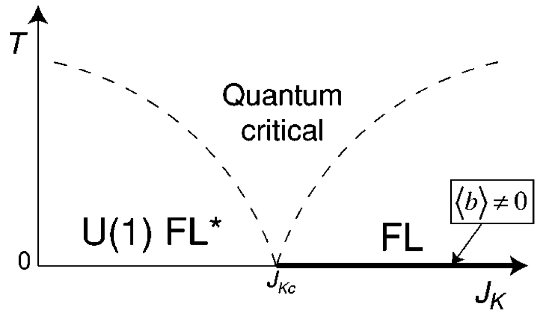
Figure 1: Crossover phase diagram for the Kondo breakdown transition. In this paper, we analyze transport properties in the $U(1)$ FL^∗ phase. Upon increasing temperature in this phase, transport properties are expected to show a crossover due to the fluctuating bosonic hybridization field $b_{i}^{\dagger}$ in the quantum critical region. Figure taken from Ref. senthil04, .

The action $S_{f}+S_{a}$ has been discussed in many different contexts.nagaosarmp Here, we consider it as a starting point in order to analyze physical observables of the FL^∗ phase.

III General transport properties

III.1 Linear response

We are interested in the response of the total electrical current density ${\bf J}$ and the total heat current density ${\bf Q}$ to an applied electrical field ${\bf E}$ and a temperature gradient ${\vec{\nabla}}T$, weak enough in order to linearize ${\bf J}$ and ${\bf Q}$ in the applied fields. These properties may be formulated individually for each type of particle, which we label by $\alpha=b,c,f$ for bosons, conduction electrons and spinons, respectively. The transport coefficients for these individual types of particles are defined by the relations

$${\bf J}_{\alpha} = \kappa_{0\alpha}({\bf E}_{\alpha}-\vec{\nabla}\mu_{\alpha})+\kappa_{1\alpha}\biggl{[}\frac{-\vec{\nabla}T}{T}\biggr{]}$$

$${\bf Q}_{\alpha} = \kappa_{1\alpha}({\bf E}_{\alpha}-\vec{\nabla}\mu_{\alpha})+\kappa_{2\alpha}\biggl{[}\frac{-\vec{\nabla}T}{T}\biggr{]}\ ,$$ (4)

where the Onsager relation for thermoelectrical transport coefficients has been used.ziman60 The field coupling to the electrical transport coefficient $\kappa_{0\alpha}$ can originate both from an electrical field or a gradient in the chemical potential. Precise definitions for the current densities ${\bf J}$ and ${\bf Q}$ will appear in concrete calculations in Section IV. The thermal conductivity $\kappa$ is defined by the relation ${\bf Q}=-\kappa\vec{\nabla}T$ with the boundary condition ${\bf J}=0$. This implies that in general, the total thermal conductivity $\kappa$ will depend on all of the coefficients entering Eq. (4). This complicated dependence can be slightly simplified by rewriting the thermal conductivity in form of a variational functional as described by Ziman,ziman60 such that not all of the $9$ coefficients $\kappa_{\{0,1,2\}\alpha}$ need to be evaluated explicitly. We will introduce this approach in explicit calculations later on. Moreover, any concrete calculation becomes simplified considerably if the contribution of conduction electron and spinon degrees of freedom to the total thermal conductivity can be calculated separately. This case is not justified in general, since Eq. (4) couples different electrical fields ${\bf E}_{\alpha}$ to each type of particle. More precisely, corrections to the approximation of independent spinon and conduction electron thermal currents arise for temperatures above or the same size as the crossover temperature T^∗ related to the boson mass gap $\mu_{b}$. A formal discussion of transport properties in this general situation can be given in terms of the composition rules first discussed by Ioffe and Larkin.ioffe89 ; pepin08

III.2 Ioffe-Larkin rules

The fact that the boson variable $b_{i}^{\dagger}$ is given by $b_{i}^{\dagger}=\sum_{\sigma}f_{i\sigma}^{\dagger}c_{i\sigma}^{\phantom{\dagger}}$ immediately implies the relation $\mu_{b}=\mu_{f}-\mu_{c}$ between the chemical potentials of boson and fermions, while the electrical fields felt by the particles are

$${\bf E}_{b}={\bf e}-{\bf E}\qquad{\bf E}_{f}={\bf e}\qquad{\bf E}_{c}={\bf E}\ .$$ (5)

Here, the electrical field ${\bf e}$ is the fictitious field strength felt by the gauge charge of a spinon in presence of a finite external electrical field ${\bf E}$. Since both bosons and spinons couple to the internal gauge field ${\bf a}$, the gauge current densities will fulfill the constraint ${\bf J}_{b}+{\bf J}_{f}=0$. The physical electrical current density is given by ${\bf J}={\bf J}_{c}+{\bf J}_{b}$. From these constraints, one can readily derive the composition rules stated in Ref. kim09, , representing extensions to the composition rules of Ioffe and Larkin.ioffe89 For the total thermal conductivity $\kappa_{t}$, these rules imply the formkim09

$$\frac{\kappa_{t}}{T}=\frac{\kappa_{2c}}{T}+\frac{\kappa_{2f}}{T}+\frac{\kappa_{2b}}{T}-\frac{(\kappa_{1b}+\kappa_{1f})^{2}}{\kappa_{0b}+\kappa_{0f}}-\frac{\kappa_{1t}^{2}}{\kappa_{0t}}\ .$$ (6)

Here, $\kappa_{0t}$ is the total electrical conductivity and $\kappa_{1t}$ the total thermoelectric conductivity. The correction terms $\frac{\kappa_{2b}}{T}-\frac{(\kappa_{1b}+\kappa_{1f})^{2}}{\kappa_{0b}+\kappa_{0f}}$ become exponentially small as a function of temperature below the crossover temperature scale following $T^{\ast}\sim|\mu_{b}|^{2/3}$ in three dimensions,senthil04 since the number of bosons decreases exponentially as function of temperature in this regime. In the same way, $\kappa_{0t}$ and $\kappa_{1t}$ reduce to the conduction electron contributions $\kappa_{0c}$ and $\kappa_{1c}$, since the spinons carry no physical electrical charge. It might be possible instead to measure the spin conductivity of the spinons, which shows a temperature dependence identical to the gauge charge conductivity. Its temperature-dependence behaves as $\sim T^{5/3}$ in three spatial dimensions.kim10 We do not elaborate on the spin conductivity as it is a rather complicated quantity to be measured experimentally.

Above the crossover scale T^∗, the presence of hybridization bosons provides both a strong source of scattering and a sizable channel for heat conduction, and we cannot neglect their contribution to transport observables. Throughout the following calculations, we assume that $T<T^{\ast}$ and neglect therefore the presence of the hybridization boson degrees of freedom. Therefore, we can assume that the conduction electron system shows conventional Fermi liquid properties, while the spinon system will be responsible for non-Fermi liquid properties.

III.3 Spinon self-energy

In order to analyze scattering processes of spinons on gauge field fluctuations, it is convenient to consider the transverse gauge, $\nabla\cdot{\bf a}=0$. In this case, the scalar ($a_{0}$) and transverse parts of the gauge field fluctuations decouple. $a_{0}$ corresponds to a density-density response function and does not lead to singular corrections to the spinon dynamics.nagaosarmp It is therefore possible to concentrate on the transverse fluctuations. The spinon self-energy due two single gauge boson exchange processes has been discussed by many authors.gan93 ; nagaosarmp Close to the spinon Fermi surface, the spinon self-energy corrections are

$$\Sigma_{a}({\bf k},\omega)=\lambda_{1}|\omega|^{2/3}\text{sgn}(\omega)+i\lambda_{2}|\omega|^{2/3}$$ (7)

in $2d$ and

$$\Sigma_{a}({\bf k},\omega)=\lambda_{1}\omega\ln\biggl{(}\frac{\Lambda}{\omega}\biggr{)}+i\lambda_{2}\omega$$ (8)

in $3d$.gan93 Here, $\lambda_{1}$ and $\lambda_{2}$ are constants that depend on details of the spinon Fermi surface. Due to these self-energy corrections, the quasiparticle lifetime is not much longer than its inverse energy and several non-Fermi liquid properties result both in two and in three spatial dimensions.gan93 An additional complication arises at finite temperatures, since $\Sigma_{a}({\bf k},\omega)$ is divergent in $d\leq 3$ for $\omega<T$.nagaosarmp In order to describe transport properties of the coupled system of spinons and gauge field, Kim et al. formulated a quantum Boltzmann equation approach in which the low energy fluctuations of the gauge field are split off from the collision integral in order to avoid the divergent self-energy.kim95
To cure the finite temperature divergence of the single-particle self-energy, vertex corrections are of central importance. The divergence mentioned above is caused by the fact that the single-particle spinon Green’s function is not invariant under a U(1) gauge transformation.nagaosarmp In order to calculate a gauge invariant quantity such as thermal conductivity, it is also possible to include the low-energy gauge fluctuations into a quantum Boltzmann equation, since the divergences are expected to cancel in the gauge invariant conductivities. This situation occurs in our following calculations.

At low frequencies the spinons are also influenced by impurity scattering for which we assume potential scattering with potential strength $V({\bf r})$. Any type of impurity with short-ranged Coulomb potential will lead to such scattering processes. We assume in the following that the scattering potential is independent of temperature, as well as a temperature independent concentration and a Gaussian distribution of impurities in the bulk of the sample. Modifications to the impurity potential are expected to occur only at temperatures of order the ionization energy required to change the impurity charge, which is considerably higher than room temperature. To lowest order in the impurity concentration $n_{i}$, such impurity scattering processes are described bymahan90

$$\Sigma_{\text{imp}}({\bf k},\omega)=n_{i}T_{{\bf k}{\bf k}}$$ (9)

with the $T$-matrix given by the solution to

$$T_{{\bf k}{\bf k}^{\prime}}(\omega)=V({\bf k}-{\bf k}^{\prime})+\int\frac{d^{3}{\bf p}}{(2\pi)^{3}}\frac{V({\bf k}-{\bf p})T_{{\bf p}{\bf k}^{\prime}}(\omega)}{\omega-\xi_{\bf p}+i\delta}\ .$$ (10)

Here, $\xi_{\bf p}={\bf p}^{2}/(2m_{f})-\mu$ is the spinon dispersion and $V({\bf p})$ is the Fourier transform of $V({\bf r})$. In the following, we neglect interference processes between scattering on gauge bosons and impurities, such that the total self-energy is given by $\Sigma({\bf k},\omega)=\Sigma_{\text{imp}}({\bf k},\omega)+\Sigma_{a}({\bf k},\omega)$. This approximation is valid if the mean free path derived from one of these two collision processes is much larger than that of the second collision process. Since the mean free path is given by the spinon Fermi velocity times the spinon lifetime $v_{F}/\Sigma({\bf k}_{\bf F},\omega)$, it is sufficient to compare the size of the two self-energy contributions $\Sigma_{\text{imp}}({\bf k},\omega)$ and $\Sigma_{a}({\bf k},\omega)$ for this purpose. Setting them equal defines a characteristic temperature which we denote by $T_{1}$. First, the neglect of interference processes is therefore valid in the temperature regime $T_{1}\ll T<T^{\ast}$ where scattering on gauge field fluctuations dominates, such that $\Sigma({\bf k},\omega)\simeq\Sigma_{a}({\bf k},\omega)$. The temperature scale $T^{\ast}$ is the crossover temperature for the FL^∗ phase boundary we introduced above. Second, our approximation is also valid for temperatures $T\ll T_{1}$ where impurity scattering dominates the self energy such that $\Sigma({\bf k},\omega)\simeq n_{i}T_{{\bf k}_{\bf F}{\bf k}_{\bf F}}(\omega=0)$. The temperature scale $T_{1}$ is set by equating the imaginary parts $\Sigma^{\prime\prime}_{\text{imp}}({\bf k}_{\bf F},\omega=0)=\Sigma^{\prime\prime}_{a}({\bf k}_{\bf F},\omega)$ and considering $\hbar\omega\simeq k_{B}T$. We abbreviate the impurity self-energy as the spinon scattering rate $\tau_{f}^{-1}$ such that $\Sigma_{\text{imp}}({\bf k}_{\bf F},\omega=0)=\tau_{f}^{-1}$. For the constant $\lambda_{2}$ in Eqs (7) and (8), we use the estimate $\lambda_{2}\simeq(\epsilon_{F}^{f})^{1/3}$ in 2d.blok93 In 3d, an estimate for metals is given by $\lambda_{2}\simeq 10^{-5}$,kwon95 although the gauge field coupling of the spinons can differ to some extend from the case of electrons in a metal. In this way, we obtain

$$k_{B}T_{1}\simeq\biggl{[}\frac{\hbar}{\tau_{f}(\epsilon_{F}^{f})^{\frac{1}{3}}}\biggr{]}^{3/2}$$ (11)

in $2d$ and

$$k_{B}T_{1}\simeq 10^{5}\frac{\hbar}{\tau_{f}}$$ (12)

in $3d$. We thus conclude that the temperature window where the neglect of interference processes is not justified is proportional to $\tau_{f}^{(d-5)/2}\sim n_{i}^{(5-d)/2}$ and therefore shrinks rapidly with decreasing impurity concentration. Concise numbers for the temperature $T_{1}$ can obtained by estimating $\tau_{f}$ from the residual conductivity expression (35), which itself could be estimated from the conduction electron residual conductivity. Another way to check the justification of the neglect of interference processes is to compare the mean spacing between impurities and the scattering length on gauge bosons. The latter will shrink as a function of increasing temperature and can thereby become much smaller than the mean spacing between impurities.

IV Quantum Boltzmann equation

For a fermionic quantum many-body system under non-equilibrium conditions, we define the usual Keldysh propagators mahan90

$$G^{>}(x_{1},x_{2}) = -i\langle\psi(x_{1})\psi^{\dagger}(x_{2})\rangle$$

$$G^{<}(x_{1},x_{2}) = i\langle\psi^{\dagger}(x_{1})\psi^{\phantom{\dagger}}(x_{2})\rangle$$

$$G_{t}(x_{1},x_{2}) = \theta(t_{1}-t_{2})G^{>}(x_{1},x_{2})$$

$$+ \theta(t_{2}-t_{1})G^{<}(x_{1},x_{2})$$

$$G_{\bar{t}}(x_{1},x_{2}) = \theta(t_{2}-t_{1})G^{>}(x_{1},x_{2})$$ (13)

$$+ \theta(t_{1}-t_{2})G^{<}(x_{1},x_{2})$$

and formulate a Dyson equation

$$\tilde{G}=\tilde{G}_{0}+\tilde{G}_{0}\tilde{\Sigma}\tilde{G}$$ (14)

for the matrix Green’s function

$$\tilde{G}=\left[\begin{array}[]{cc}G_{t}&-G_{<}\\ G_{>}&-G_{\bar{t}}\\ \end{array}\right]$$ (15)

and $\tilde{\Sigma}$ defined in analogy. $\tilde{G}_{0}$ contains the non-interacting propagators. We employed the combined variable $x=({\bf r},t)$ that parametrizes the fermionic field $\psi$. Without further complications, it can also include spin and other variables. For brevity, we dropped these coordinates in Eqs (14) and (15) as well as we dropped integrating over intermediate coordinates in Eq. (14).
For transport processes, it is convenient to introduce a center-of-mass coordinate system

$$({\bf R},T) = \frac{1}{2}(x_{1}+x_{2})$$

$$({\bf r},t) = x_{1}-x_{2}\ .$$ (16)

Starting from the Dyson equation (14) it is then possible to derive an equation of motion for $G^{<}(x_{1},x_{2})$, which we refer to as quantum Boltzmann equation. This has been discussed in detail by Mahan.mahan90 For these purposes, it is convenient to work in the Fourier space of relative coordinates ${\bf r}$

$$\tilde{G}({\bf k},\omega,{\bf R},T)=\int d^{d}{\bf r}e^{i{\bf k}{\bf r}}\int dte^{i\omega t}\tilde{G}({\bf r},t,{\bf R},T)\ .$$ (17)

IV.1 Derivation

Our transport description starts from the gauge invariant quantum Boltzmann equation mahan90

$$i \biggl{\{}\frac{\partial}{\partial T}+{\bf v}_{\bf k}\cdot\nabla_{\bf R}+e{\bf E}\cdot\biggl{[}\biggl{(}1-\frac{\partial\text{Re}\Sigma_{\text{ret}}}{\partial\omega}\biggr{)}\nabla_{\bf k}$$ (18)

$$+ ({\bf v}_{\bf k}+\nabla_{\bf k}\text{Re}\Sigma_{\text{ret}})\frac{\partial}{\partial\omega}\biggr{]}\biggr{\}}G^{<}-ie{\bf E}\cdot\biggl{[}\frac{\partial\Sigma^{<}}{\partial\omega}\nabla_{\bf k}\text{Re}G_{\text{ret}}$$

$$- \frac{\partial\text{Re}G_{\text{ret}}}{\partial\omega}\nabla_{\bf k}\Sigma^{<}\biggr{]}=\Sigma^{>}G^{<}-\Sigma^{<}G^{>}$$

$$+ i[\text{Re}\bigl{[}\Sigma_{\text{ret}}\bigr{]},G^{<}]+i[\Sigma^{<},\text{Re}\bigl{[}G_{\text{ret}}\bigr{]}]\ .$$

Here, we employed the Poisson bracket

$$[\Sigma,G] = \frac{\partial\Sigma}{\partial\omega}\frac{\partial G}{\partial T}-\frac{\partial\Sigma}{\partial T}\frac{\partial G}{\partial\omega}$$ (19)

$$- \nabla_{\bf k}\Sigma\cdot\nabla_{\bf R}G+\nabla_{\bf R}\Sigma\cdot\nabla_{\bf k}G$$

and used the retarded propagator $G_{\text{ret}}$ defined by the relation $G_{\text{ret}}=G_{t}-G^{<}$. Further simplifications to Eq. (18) can be made in absence of an external electrical field (${\bf E}=0$), such that all terms proportional to ${\bf E}$ can be dropped. In addition we linearize both hand sides in $\nabla_{\bf R}$. Here, we just state the result that we justify further in Appendix A,

$$A\frac{\partial f}{\partial\omega}\frac{\nabla_{\bf R}T}{T}\cdot{\bf v}_{\bf k}\omega=\Sigma^{>}G^{<}-\Sigma^{<}G^{>}\ .$$ (20)

In the driving terms, the quantities $\Gamma=-2\text{Im}\Sigma_{\text{ret}}$, $A=i(G^{>}-G^{<})$ and the Fermi function $f(\omega)=(1+\exp(\beta\omega))^{-1}$, $\beta=1/k_{\text{B}}T$, appear. From the solution to this equation, the thermal current density is obtained as

$${\bf Q}=-i\int\frac{d^{d}{\bf k}}{(2\pi)^{3}}\frac{{\bf k}}{m_{f}}\int\frac{d\omega}{2\pi}\omega G^{<}({\bf k},\omega)\ .$$ (21)

By linearizing this equation in the driving field $\nabla_{\bf R}T$, it is possible to obtain the thermal conductivity $\kappa$ if the boundary condition ${\bf J}=0$ is obeyed.
In order to specify the collision term in Eq. (20), we consider the non-equilibrium self-energy contributions from single gauge boson exchange processes

$$\Sigma_{\text{a}}^{<}({\bf k},\omega)=\sum_{\bf q}\int_{0}^{\infty}\frac{d\nu}{\pi}\biggl{|}\frac{{\bf k}\times{\bf{\hat{q}}}}{m_{f}}\biggr{|}^{2}\text{Im}D({\bf q},\nu)\biggl{[}\{n(\nu)+1\}$$

$$G^{<}({\bf k}+{\bf q},\omega+\nu)+n(\nu)G^{<}({\bf k}+{\bf q},\omega-\nu)\biggr{]}\ ,$$ (22)

and the contribution from potential scattering

$$\Sigma_{\text{imp}}^{<}({\bf k},\omega)=n_{i}\int\frac{d^{3}{\bf p}}{(2\pi)^{3}}[T_{{\bf k}{\bf p}}(\omega)]^{2}G^{<}({\bf p},\omega)\ .$$ (23)

The total self-energy is given by the sum $\Sigma^{<}=\Sigma_{\text{a}}^{<}+\Sigma_{\text{imp}}^{<}$. We note that in this approximation, we have approximated the gauge field propagator by its equilibrium form. This approximation implies that the presence of a thermal current of gauge bosons does not change the spinon thermal conductivity. No contradiction with previous approximations arises. Although without impurities, the system has the translational symmetries of the Bravais lattice, the finite spinon thermal conductivity we will obtain within the approximation of an equilibrated gauge field is not artificial. A well-known analogy is the electrical conductivity of a Fermi liquid, which has a well-established temperature dependence that can be obtained from scattering due to quasiparticle interactions, without involving mechanisms that break translational invariance. We will comment further on this approximation when we discuss the thermal conductivity of the gauge bosons.

IV.2 Variational principle

It turns out that Equation (20) is too complicated to solve in this form. We attempt to simplify it further such that it can be rewritten in form of a variational principle for the distribution function $G^{<}({\bf k},\omega)$. We make the linearized ansatz

$$G^{<}({\bf k},\omega)=iA({\bf k},\omega)\biggl{[}f(\omega)-\frac{\partial f(\omega)}{\partial\omega}\frac{\nabla_{\bf R}T}{T}\cdot{\bf v}_{\bf k}\Lambda({\bf k},\omega)\biggr{]}\ ,$$ (24)

which is valid in the regime $\bigl{|}\nabla_{\bf R}T/T\bigr{|}\ll 1$. All non-equilibrium properties are encoded in the vertex distribution function $\Lambda({\bf k},\omega)$ which still needs to be determined. First, we assume that the collision term is dominated by scattering on the gauge field, $\Sigma_{a}^{<}\gg\Sigma_{\text{imp}}^{<}$. This approximation is valid in the temperature regime $T_{1}\ll T<T^{\ast}$ discussed above. Employing Eqs (22) and (24), the collision term can be specified as

$$i[\Sigma^{<}A-2\Gamma G^{<}]=2\Gamma({\bf k},\omega)A({\bf k},\omega)\frac{\partial f}{\partial\omega}\frac{\nabla_{\bf R}T}{T}\cdot{\bf v}_{\bf k}\Lambda({\bf k},\omega)$$ (25)

$$+ A({\bf k},\omega)\sum_{\bf q}\int_{0}^{\infty}\frac{d\nu}{\pi}\biggl{|}\frac{{\bf k}\times\hat{{\bf q}}}{m_{f}}\biggr{|}^{2}\text{Im}D({\bf q},\nu)\biggl{[}\frac{\nabla_{\bf R}T}{T}\cdot{\bf v}_{{\bf k}+{\bf q}}\biggr{]}$$

$$\frac{\partial f(\omega)}{\partial\omega}\biggl{\{}[n(\nu)+f(\omega+\nu)]\frac{1-f(\omega+\nu)}{1-f(\omega)}$$

$$A({\bf k}+{\bf q},\omega+\nu)\Lambda({\bf k}+{\bf q},\omega+\nu)-[n(-\nu)+f(\omega-\nu)]$$

$$\frac{1-f(\omega-\nu)}{1-f(\omega)}A({\bf k}+{\bf q},\omega-\nu)\Lambda({\bf k}+{\bf q},\omega-\nu)]\biggl{\}}\ .$$

Solving this equation for the vertex distribution function yields the self-consistency condition

$$\Lambda({\bf k},\omega)=\frac{\omega}{2\Gamma({\bf k},\omega)}-\frac{1}{2\Gamma({\bf k},\omega)}\sum_{\bf q}\int_{0}^{\infty}\frac{d\nu}{\pi}\biggl{|}\frac{{\bf k}\times{\hat{{\bf q}}}}{m_{f}}\biggr{|}^{2}$$

$$\text{Im}D({\bf q},\nu)\frac{{\bf v}_{{\bf k}+{\bf q}}\cdot{\bf v}_{{\bf k}}}{v_{\bf k}^{2}}\biggl{\{}[n(\nu)+f(\omega+\nu)]\frac{1-f(\omega+\nu)}{1-f(\omega)}$$

$$A({\bf k}+{\bf q},\omega+\nu)\Lambda({\bf k}+{\bf q},\omega+\nu)-[n(-\nu)+f(\omega-\nu)]$$

$$\frac{1-f(\omega-\nu)}{1-f(\omega)}A({\bf k}+{\bf q},\omega-\nu)\Lambda({\bf k}+{\bf q},\omega-\nu)\biggr{\}}\ .$$ (26)

Equation 26 is solved by a vertex distribution function $\Lambda(\omega)$ that depends only on frequency but not on momentum. This result is of central importance in order to formulate a variational ansatz for $G^{<}({\bf k},\omega)$ later on. To begin with, $\Gamma({\bf k},\omega)$ does not depend on momentum according to Eqs (7) and (8), such that $A({\bf k}+{\bf q},\omega)$ depends on ${\bf k}$ only through the variable $\xi=\epsilon_{{\bf k}+{\bf q}}-\mu$. The collision integral is dominated by gauge boson frequencies $\nu\simeq q^{3}\chi_{d}/\Gamma$, with the frequency being set by $\nu\simeq k_{B}T$. In the limit $k_{B}T\ll k_{F}^{3}\chi_{d}/\Gamma\simeq\epsilon_{F}^{f}$, we can therefore approximate $q\ll k_{F}$, such that all other terms in the integrand of Eq. (26) approximately depend only on $q$ but not on ${\bf k}$, with corrections of higher order in the small parameter $q$. We will give an estimate for the spinon Fermi energy $\epsilon_{F}^{f}$ below. Within this approximation, the integral can be entirely parametrized in terms of the variables $\xi=\epsilon_{\bf k+q}-\mu$ and $q$, and the value of the integral will not depend on ${\bf k}$. Therefore, $G^{<}({\bf k},\omega)$ will depend on the variable $\xi=\epsilon_{\bf k}-\mu$ only through the equilibrium spectral function $A({\bf k},\omega)$, which is sharply peaked as a function of $\xi$. This variable can therefore be eliminated from the quantum Boltzmann equation, and we can make use of the reduced distribution function

$$f(\hat{{\bf k}},\omega)=-i\int\frac{d\xi}{2\pi}G^{<}(\xi,\hat{{\bf k}},\omega)\ .$$ (27)

In this case, it is possible to represent the thermal conductivity as a variational functional.ziman60 A similar approach has been employed previously by Nave and Lee nave07 in the case of two dimensions. We repeat their steps wherever it is instructive in order to understand our results for the three dimensional case.

Introducing an ansatz of the form $f(\hat{{\bf k}},\omega)=f(\omega)-\phi(\hat{{\bf k}},\omega)\frac{\partial f}{\partial\omega}$ immediately leads to

$$\phi(\hat{\bf k},\omega)\sim\frac{\nabla_{\bf R}T}{T}\cdot{\bf v}_{{\bf k}}\Lambda(\omega)\ .$$ (28)

Assuming a power-law dependence $\Lambda(\omega)\propto\omega^{s}$,foot3 the trial function is given by $\phi(\hat{{\bf k}},\omega)=\omega\hat{{\bf k}}(\nabla_{\bf R}T/T)$. Upon inserting the definitions for $\dot{S}$ and ${\bf Q}$ into the general form of Eq. (30), it is seen that the power $s$ in the ansatz $\Lambda(\omega)\propto\omega^{s}$ drops out of the temperature dependence of the thermal conductivity once frequency is rescaled with temperature. Therefore, we dropped the exponent $s$ from our variational ansatz. Note that it is not necessary to normalize $\phi(\hat{{\bf k}},\omega)$ since the normalization constant will drop out of our final results. We next define the rate of entropy density production as

$$\dot{S}=\vec{\nabla}\biggl{(}\frac{1}{T}\biggr{)}\cdot{\bf Q}$$ (29)

generated by the thermal current density ${\bf Q}$. $\phi$ minimizes the variational functional

$$W=\frac{T^{2}\dot{S}}{Q^{2}}\ ,$$ (30)

where ${\bf Q}$ is the heat current density given by

$${\bf Q}=N(0)\int d\hat{\bf k}d\omega\phi v_{F}\omega\frac{\partial f_{0}}{\partial\omega}{\bf\hat{k}}$$ (31)

and the rate $\dot{S}$ of entropy density production is

$$\dot{S} = \frac{N_{0}^{2}}{m_{f}^{2}}\beta^{2}\int d\omega d\omega^{\prime}d\nu d{\bf q}d\hat{{\bf k}}d\hat{{\bf k}}^{\prime}|{\bf k}^{\prime}\times\hat{{\bf q}}|^{2}$$ (32)

$$\times {\text{Im}}D({\bf q},\nu)(\phi-\phi^{\prime})^{2}f_{0}(\omega)[1-f_{0}(\omega^{\prime})]n_{0}(\nu)$$

$$\times \delta(\omega^{\prime}-\omega-\nu)\delta((\hat{{\bf k}}^{\prime}-\hat{\bf k})-\frac{\bf q}{k_{F}})\ .$$

Here the integration over ${\bf\hat{k}}$ is defined as integration over the $d-1$ dimensional unit sphere, $N(0)$ is the density of states at the Fermi level for up and down spins combined. In $2d$, we have $N(0)=m_{f}/\pi$ and in 3d $N(0)=m_{f}k_{F}/(2\pi^{2})$ The global minimum of the variational functional $W$ is identical to the spinon thermal resistivity $\kappa_{f}^{-1}$.
As discussed in Section III.3, at lowest temperatures the energy relaxation rate is impurity dominated

$$\Gamma({\bf k},\omega)\sim 2\Gamma_{0}\ ,$$ (33)

assuming a constant impurity contribution $2\Gamma_{0}=2n_{i}\text{Im}\bigl{[}T_{{\bf k_{F}}{\bf k_{F}}}(\omega=0)\bigr{]}$. In this case, the rate of entropy density production in Eq. (32) has to be modified accordingly. Instead, this case can be treated in a much simpler way by using the Wiedemann-Franz law for free fermions

$$\frac{\kappa_{f}}{\kappa_{0f}T}=L_{0}\ ,$$ (34)

with the Lorentz number $L_{0}=(\pi^{2}/3)(k_{B}/e)^{2}$. We can use the Drude formula for the residual conductivity of a Fermi gas

$$\kappa_{0f}=\frac{n_{f}e^{2}\tau_{f}}{m_{f}}$$ (35)

and insert it into Eq. (34) to determine the spinon heat conductivity $\kappa_{f}$. The spinon density $n_{f}$ is equal to the inverse unit cell volume, while the spinon scattering rate $\tau_{f}^{-1}$ can be equated to twice the self-energy correction from impurity scattering, $2\Gamma_{0}$. Independent of dimension, up to a number of $\mathcal{O}(1)$, the heat current density is given by $Q\equiv N(0)v_{F}(k_{B}T)^{2}$.
In order to determine $\dot{S}$ in Eq. (32), we first integrate over the variables $\omega,\omega^{\prime}$ and ${\bf q}$ and parametrize the integrals over $\hat{{\bf k}}$ and $\hat{{\bf k}}^{\prime}$ in spherical coordinates. Furthermore, we can approximate

$$(\phi-\phi^{\prime})^{2}=\nu^{2}({\hat{\bf k}\cdot\hat{\bf u}})^{2}+2\nu(\omega-\mu)^{2}\mathcal{O}(q)\ ,$$ (36)

where $\nu$ is given by the relative frequency $\nu=\omega-\omega^{\prime}$. Since the main contribution to the integral comes from $q\sim\nu^{1/3}$, the term $\nu^{2}({\hat{\bf k}\cdot\hat{\bf u}})^{2}$ dominates the temperature dependence at $k_{B}T\ll\epsilon_{F}^{f}$ and we can neglect the term $2\nu(\omega-\mu)^{2}\mathcal{O}(q)$ and all higher corrections. A straightforward but somewhat tedious integration shows then that the rate of entropy production follows $\dot{S}\sim(k_{B}T)^{(6+d)/3}$.
We note that we did not introduce an infrared cutoff frequency for the gauge field mode in Eq. (32), although this leads to a divergent retarded self-energy at finite temperatures.nagaosarmp Even at one loop order, this divergence is canceled in the collision integral of the QBE. Introducing an infrared cutoff given by $\beta\nu=1$ would only renormalize the prefactor of the overall result by a number of $\mathcal{O}(1)$, as we checked explicitly.

IV.3 Thermal conductivity: results

Putting together the Drude result and the result for scattering on gauge bosons, the spinon conductivity is given by

$$\frac{\kappa_{f}}{T}=\left\{\begin{array}[]{cc}\biggl{[}\frac{\hbar}{k_{B}^{2}}\bigl{(}\frac{k_{B}T}{\epsilon_{F}^{f}}\bigr{)}^{2/3}+\frac{3}{\pi^{2}}\frac{m_{f}}{k_{B}^{2}n_{f}\tau_{f}}\biggr{]}^{-1}\quad(2d)\\ \biggl{[}\frac{\hbar}{k_{B}^{2}}\frac{k_{B}T}{k_{F}\epsilon_{F}^{f}}+\frac{3}{\pi^{2}}\frac{m_{f}}{k_{B}^{2}n_{f}\tau_{f}}\biggr{]}^{-1}~{}\qquad\quad(3d)\end{array}\right\}\ .$$ (38)

(39)

Here, we restored units of $\hbar$ and $k_{B}$ and omitted prefactors of $\mathcal{O}(1)$. The spinon density $n_{f}$ corresponds simply to the inverse of the unit cell volume, such that $n_{f}=1/V_{uc}$. We defined the unit cell volume $V_{uc}$ as the volume of the two-dimensional unit cell for the two-dimensional thermal conductivity and as the volume of the three-dimensional unit cell for the three-dimensional thermal conductivity. Therefore, we defined the two-dimensional thermal conductivity as the thermal conductivity of a single two-dimensional layer. It turns out from the results in Eq. (39) that in both two and three dimensions, the spinon thermal conductivity agrees with the basic argument $\kappa\sim C_{V}v_{F}^{2}\tau_{E}$ stated by Nave and Lee,nave07 assuming that the specific heat follows $C_{V}\sim\gamma T$ and $\tau_{E}$ is the energy relaxation rate of the spinons, which is constant for isotropic impurity scattering and follows $\tau_{E}\sim T^{-d/3}$ for scattering on gauge field fluctuations.nagaosarmp The result for the two-dimensional thermal conductivity has been already obtained by Nave and Lee.nave07 For the case of three-dimensional candidate materials, we have now obtained the finding that the thermal conductivity of the spinons due to scattering on gauge field fluctuations has a temperature- independent contribution. This can be seen from the result for 3d in Eq. (39), since $\kappa_{f}/T\sim 1/T$ in the limit $\tau_{f}^{-1}=0$. However, due to impurity scattering the total thermal conductivity will vanish in the limit of zero temperature, such that the constant term $d_{2}$ appearing in Table 1 can only appear above the temperature scale $T_{1}$ introduced in 1.

	(I) $T\ll T_{1}$	(II) $T_{1}\ll T<T_{2}$	(III) $T_{2}<T$
2d	$c_{1}T$	$c_{2}T^{1/3}$	non-universal
3d	$d_{1}T$	$d_{2}$	non-universal

Table 1: Temperature-dependence of the total thermal conductivity $\kappa$ in different temperature regimes. Estimates for the characteristic temperatures $T_{1}$ and $T_{2}$ as well as expressions for the parameters $c_{1}$, $c_{2}$, $d_{1}$ and $d_{2}$ are discussed in the main text. The temperature-dependence in regime (III) is non-universal since it depends also on the temperature scale $T^{\ast}$, among other aspects. It is discussed in more detail in the main text.

It is important to recall that we have approximated the collision integral by the sum of impurity and gauge field collision processes, and it has been assumed that any interference between these types of collision processes does not influence the temperature dependence of the spinon thermal conductivity.

Finally, the contribution of conduction electrons to the thermal conductivity can be obtained by using the Wiedemann-Franz law (34),

$$\kappa_{c}=L_{0}\rho^{-1}T,$$ (40)

with the Fermi liquid resistivity coleman

$$\rho = \rho_{0}+a\frac{h}{2e^{2}}\biggl{(}\frac{\Gamma}{2\epsilon_{F}^{c}}\biggr{)}$$

$$\Gamma = \frac{1}{2}(\pi k_{B}T)^{2}/\epsilon_{F}^{c}\ .$$ (41)

Here, $a$ is the interlayer spacing of the metallic system, $\epsilon_{F}^{c}$ the conduction electron Fermi energy and the residual resistivity $\rho_{0}$ can be determined from the Drude formula (35). In metallic systems, the Lorentz number $L_{0}$ is up to a factor of $\mathcal{O}(1)$ equivalent to the free electron value used in (34).

We now summarize the behavior of the total thermal conductivity $\kappa$ given by

$$\kappa=\kappa_{c}+\kappa_{f}\ .$$ (42)

Based on our results, we distinguish the quantitative behavior of three different temperature regimes (I)-(III) summarized in Table 1.
Regime (I) is the impurity dominated regime with a linear temperature dependence as in a conventional Fermi liquid. The ratio of spinon vs. conduction electron contribution in this regime is

$$\frac{\kappa_{f}}{\kappa_{c}}=\frac{m_{c}}{m_{f}}\frac{n_{c}\tau_{c}}{n_{f}\tau_{f}}\ .$$ (43)

$m_{c}/m_{f}$ is a small factor that is approximately given by the ratio $J_{H}/D$ of the spinon dispersion to conduction electron band width $D$. Here, $J_{H}$ is understood as the strength of nearest neighbor RKKY exchange that is naturally small compared against the conduction electron band width. This could yield to a dominance of the conduction electron contribution to the impurity dominated thermal conductivity, although the relaxation times also play a role in this ratio.
Regime (II) is the non-Fermi liquid regime dominated by the temperature dependence of the spinon contribution which extends from $T_{1}$ to some larger temperature scale $T_{2}$. It shows a rather sluggish $T^{1/3}$ dependence in two dimensions and a constant contribution in three dimensions. The temperature-dependence in regime (III) depends on various degrees of freedom, such that the temperature scale $T_{2}$ depends not only on parameters of the spinon system. First, the leading temperature dependence of the spinon thermal conductivity in regime (II) is only valid at temperatures $k_{B}T<\epsilon_{F}^{f}$, as we explained in the context of equation (26). Next, spinon scattering on hybridization bosons can only be neglected below the temperature scale $T^{\ast}$. We note that also gauge bosons carry a finite thermal current that leads to corrections to the total thermal conductivity. As discussed below, this correction is again negligible for temperatures $k_{B}T<\epsilon_{F}^{f}$. We can estimate the spinon Fermi energy $\epsilon_{F}^{f}$ by equating it to the typical energy scale $J_{H}$ for RKKY exchange interaction, $\epsilon_{F}^{f}\approx J_{H}\approx 100K$. Finally, the temperature dependence of the conduction electron contribution has to be compared against the temperature dependence of the spinon thermal conductivity. We use the estimate

$$\biggl{[}\frac{\epsilon_{F}^{c}}{k_{B}T}\biggr{]}^{2}=\biggl{[}\frac{\epsilon_{F}^{f}}{k_{B}T}\biggr{]}^{\frac{d}{3}}$$ (44)

for the temperature scale when both contributions become equal and obtain $k_{B}T=\epsilon_{F}^{c}\bigl{(}\epsilon_{F}^{f}/\epsilon_{F}^{c}\bigr{)}^{(d-1)/2}$. Since $\bigl{(}\epsilon_{F}^{f}/\epsilon_{F}^{c}\bigr{)}\ll 1$, this temperature scale is much larger than the conduction electron Fermi energy, which is of order $10^{4}$K, and we can therefore neglect the temperature dependence of the conduction electron thermal conductivity in this case. We conclude that the temperature scale $T_{2}$ is given by the minimum of the energy scales $\epsilon_{F}^{f}$ and $T^{\ast}$.
A more detailed discussion of regime (III) relies on additional high energy degrees of freedom that we excluded from our theory so far, and a more detailed analysis of this temperature regime is required to accurately discuss the thermal conductivity beyond the temperature scale $T_{2}$.

IV.4 Wiedemann-Franz ratio

A suitable quantity to detect spinon contributions to the thermal conductivity is the Wiedemann-Franz ratio

$$L(T)=\frac{\kappa_{t}}{\sigma_{t}T}\ .$$ (45)

Due to the absence of a spinon charge current, the presence of a spinon thermal current will always imply $L(T)>\kappa_{c}/(\sigma_{c}T)$. Since in our theory the conduction electron Wiedemann-Franz ratio $\kappa_{c}/(\sigma_{c}T)$ behaves as in a Fermi liquid, the additional spinon contribution will lead to characteristic deviations from Fermi liquid behavior. In the following, we distinguish two characteristic regimes for the Wiedemann-Franz ratio that are identical to the regimes (I) and (II) for the thermal conductivity of the last subsection.
In regime (I), the impurity dominated regime, the Wiedemann-Franz ratio is given by

$$\frac{\kappa_{t}}{\sigma_{t}T}=L_{0}(1+\frac{u_{f}}{u_{c}})$$ (46)

with $u_{f}=(n_{f}\tau_{f})/m_{f}$ and $u_{c}=(n_{c}\tau_{c})/m_{c}$. The absence of a spinon electrical current causes a renormalization of the Wiedemann-Franz ratio in the impurity dominated regime that might be unobservably small, due to the small mass ratio $m_{c}/m_{f}\sim J_{H}/D\ll 1$.

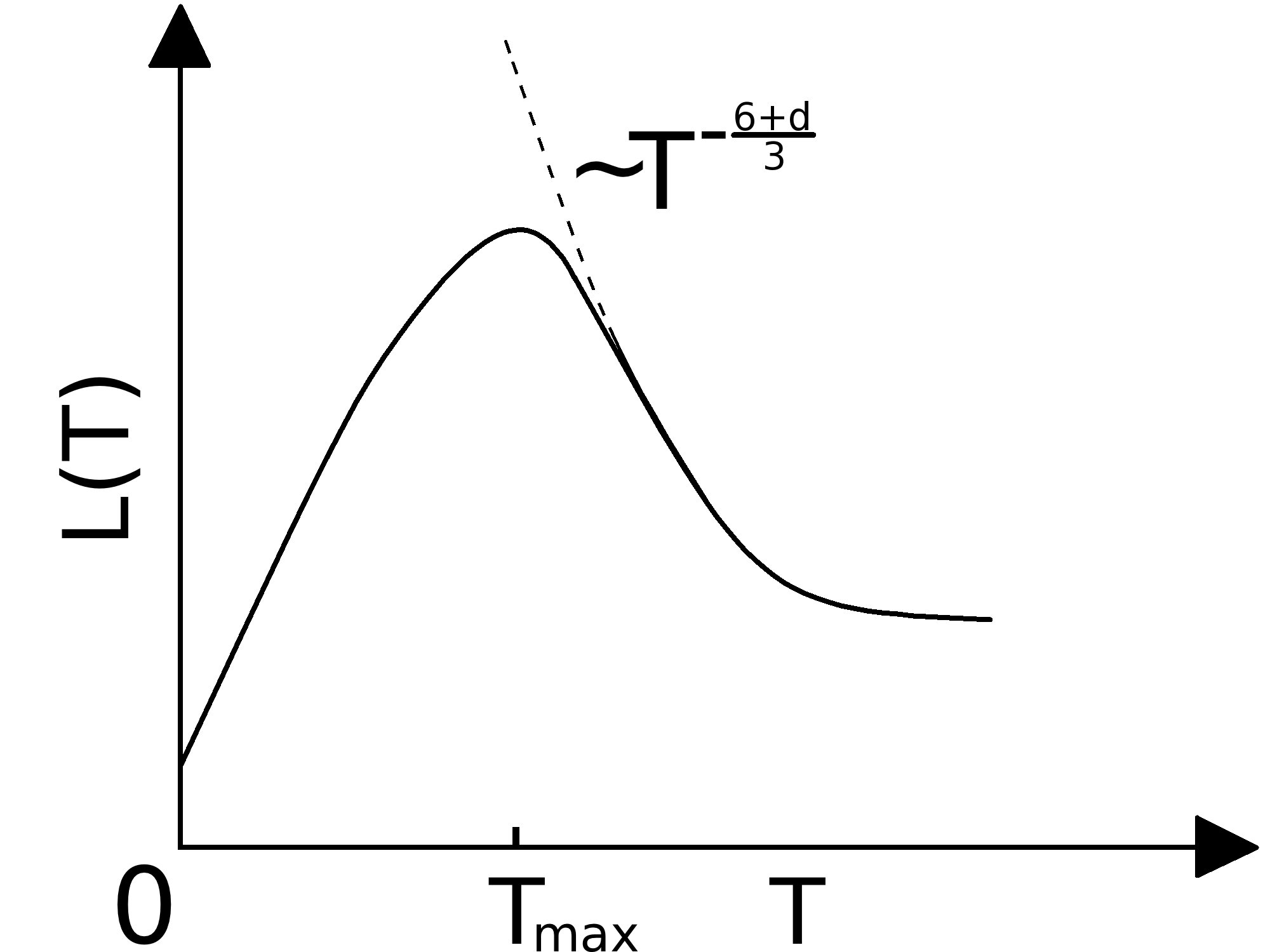
Figure 2: Sketch of the characteristic temperature dependence of the Wiedemann-Franz ratio $L(T)$ in the temperature regimes (I) and (II) discussed in the main text. The quantity $L(T)$ corresponds to the full line. At zero temperature, the ratio saturates at the finite value $L(T=0)=L_{0}(1+\frac{u_{f}}{u_{c}})$. At a temperature $T_{max}$ that is i.e. dependent on the spinon and conduction electron scattering rate, a maximum occurs that turns over into a characteristic power law divergence $T^{-(6+d)/3}$ that is sketched in form of the dashed line.

More promising with respect to observability is regime (II), where spinon collisions are dominated by scattering on gauge bosons. There, the Wiedemann-Franz ratio is given by the ratio of temperature-dependent parts of spinon thermal conductivity and conduction electron electrical conductivity. In this case the Wiedemann-Franz ratio shows the temperature dependence

$$L(T)\sim\left\{\begin{array}[]{cc}(k_{B}T)^{-\frac{8}{3}}\quad(2d)\\ (k_{B}T)^{-3}\quad(3d)\end{array}\right\}\ .$$ (48)

(49)

These divergences will be cut off at low temperatures by the thermal conductivity due to impurity scattering. Therefore, the behavior stated in Eq. (49) leads to a characteristic maximum of the Wiedemann-Franz ratio at a temperature $T_{max}$ that can be estimated by equating the two contributions to Eq. (39). This estimate results in the temperature

$$k_{B}T_{max}\simeq\biggl{[}\frac{m_{f}k_{F}(\epsilon_{F}^{f})^{2/3}}{\hbar n_{f}\tau_{f}}\biggr{]}^{\frac{3}{2}}$$

in two spatial dimensions and

$$k_{B}T_{max}\simeq\biggl{[}\frac{n_{f}k_{F}\epsilon_{F}^{f}}{\hbar m_{f}\tau_{f}}\biggr{]}$$

in three spatial dimensions. More general, any thermal conductivity with a temperature dependence dominating the Fermi liquid $T^{3}$-dependence will lead to a maximum of the Wiedemann-Franz ratio. This assumes that the electrical conductivity of the system behaves like in a Fermi liquid.

IV.5 Corrections to thermal conductivity

The contribution of gauge bosons to thermal transport can be analyzed in analogy to the spinon transport equation by defining a distribution function

$$n({\bf q},{\bf r},t)=\int\frac{d\nu}{2\pi}D^{<}({\bf q},\nu,{\bf r},t)\ .$$ (50)

It is now again possible to use the variational principle used already in this section to calculate the spinon thermal conductivity if the spinons are assumed to be in equilibrium in the gauge boson transport equation. However, in principle the gauge boson thermal current leads to a modification of the spinon thermal current and vice versa. This effect could be included by considering the coupled system of transport equations for spinons and gauge bosons. In analogy to the phonon drag in metals, such corrections to the spinon thermal conductivity can be shown to be of relative size $(k_{B}T)/\epsilon_{F}$ and can be neglected within this accuracy.ziman60 ; nave07 It is now completely analogous to the calculation of the spinon thermal conductivity to rewrite the gauge boson thermal conductivity in form of a variational functional.nave07 We do not repeat these steps in detail here, but cite just the result we obtained. After solving the integrals for the gauge boson heat current density and entropy production, the gauge boson thermal conductivity $\kappa_{g}$ can be estimated as

$$\kappa_{g}=c_{g}\biggl{[}\frac{k_{B}T}{\epsilon_{F}^{f}}\biggl{]}^{(d+1)/3}\ ,$$ (51)

with a non-universal constant $c_{g}$ that depends on details of the spinon dispersion. For temperatures $\frac{k_{B}T}{\epsilon_{F}^{f}}\ll 1$, the gauge boson thermal conductivity $\kappa_{g}$ is therefore only a subleading correction to the thermal conductivity of the spinons, see Eq. (39).
Finally, phonon contributions to the thermal conductivity are proportional to $(T/\Theta_{D})^{3}$ and are therefore negligible for temperatures much smaller than the Debye temperature $\Theta_{D}$.

V Magnetic susceptibility

V.1 Results

In our model, the physical spin susceptibility is given by the sum of the spinon susceptibility and the conduction electron susceptibility inside the FL^∗ phase,

$$\chi_{s}=\chi_{c}+\chi_{f}\ .$$ (52)

In analogy to our discussion of the thermal conductivity, corrections to this formula arise due to the presence of hybridization bosons and are therefore again exponentially small as a function of temperature below the temperature scale T^∗. We will neglect these effects in the following, considering again only temperatures $T<T^{\ast}$. Part of the behavior of the spin susceptibility $\chi_{s}$ has been discussed already by Paul et al.,paul08 with a focus mainly on the finite temperature regime above the QCP. In the FL^∗ regime considered by us, the conduction electron contribution $\chi_{c}$ is described by the usual Fermi liquid form

$$\chi_{c}=\mu_{B}^{2}\frac{2N_{c}(0)}{1+F_{0}^{a}}+\left\{\begin{array}[]{cc}b_{1}T~{}\quad(2d)\\ b_{2}T^{2}\quad(3d)\end{array}\right\}\ .$$ (54)

The paramagnetic part is controlled by the conduction electron density of states $N_{c}(0)$ at the Fermi level and the Landau parameter F${}_{0}^{a}$. Different from a Fermi gas, in two dimensions linear temperature corrections arise in a Fermi liquid,chubukov05 while in three dimensions, the usual T² dependence prevails.belitz97 The coefficients $b_{1}$ and $b_{2}$ depend on interactions and band structure details and while $b_{1}$ is positive,chubukov05 the sign of $b_{2}$ has not yet been found to the best of our knowledge. One way to obtain the spinon contribution $\chi_{f}$ is the free energy of the system of spinons and gauge field,foot4

$$F=-k_{B}T\ln Z\qquad Z=\int\mathcal{D}a\int\mathcal{D}fe^{i(S_{f}+S_{a})}\ .$$ (55)

In RPA approximation, this free energy is given by $F_{s}+F_{a}$, where $F_{a}$ is the correction to the free fermion part $F_{s}$ due to quadratic fluctuations of the transverse gauge field,

$$F_{a}=\frac{2}{\beta}\sum_{\omega_{n}}\int\frac{d^{d}k}{(2\pi)^{d}}\ln\biggl{(}\frac{\Gamma|\omega_{n}|}{k}+\chi_{d}k^{2}\biggr{)}\ .$$ (56)

Therefore, $\chi_{f}$ will have the form $\chi_{f}=\chi_{f}^{0}+\Delta\chi_{f}$, where $\chi_{f}^{0}=(g_{f}^{2}/2)\mu_{B}^{2}N_{f}(0)$ has the Fermi gas form of free spinons with g-factor $g_{f}$ and density of states at the Fermi level $N_{f}(0)$. The contribution $\Delta\chi_{f}$ denotes additional fluctuation corrections to the susceptibility.

It yet remains to discuss the dependence of $F_{a}$ on an external magnetic field. In presence of an external magnetic field, $F_{a}$ will split into two contributions $F_{a\sigma}$ stemming from different spin projections $\sigma=\pm\frac{1}{2}$. The magnetic field couples to the spinons by a Zeeman term $E_{Z}=g_{f}\mu_{B}B$ that splits the Fermi wavevector to the spin-dependent values $k_{F\sigma}=\sqrt{k_{F}^{2}+\sigma 2m_{f}E_{Z}}$, depending on the spinon g-factor $g_{f}$. In this way, it is straightforward to obtain the shift $\Delta\chi_{f}$ from

$$\Delta\chi_{f}=-\frac{\partial^{2}F_{a}}{\partial B^{2}}\biggl{|}_{B=0}\ .$$ (57)

The low temperature behavior is

$$\Delta\chi_{f}=\left\{\begin{array}[]{cc}\chi_{0}+a_{1}T^{\frac{5}{3}}\qquad\qquad~{}~{}(2d)\\ \chi_{0}+a_{2}T^{2}\log(T/\epsilon_{F}^{f})~{}(3d)\end{array}\right\}\ .$$ (59)

Details of the calculation are shown in App. B, where in particular the form of the parameters $a_{1}$ and $a_{2}$ is clarified. Both $a_{1}$ and $a_{2}$ are positive and depend on the spinon dispersion. The temperature-independent term $\chi_{0}$ is a paramagnetic contribution that has been discussed in detail in Ref. nave07b, . It is roughly of the same order of magnitude as the Pauli paramagnetic susceptibility $\chi_{f}^{0}$.

V.2 Discussion

Possibly the best way to observe the spinon contribution to the susceptibility is to consider the zero temperature limit. In this limit, the ratio of the spinon to conduction electron Pauli susceptibility is given by the ratio of their densities of states at the Fermi surface. This ratio can be estimated from the ratio of their band widths, $D/J_{H}$. The spinon band width energy scale $J_{H}$ is generated by RKKY exchange according to $J_{H}\sim J_{K}^{2}/D$, such that the spinon Pauli susceptibility dominates that of the conduction electrons by a large factor $D^{2}/J_{K}^{2}\gg 1$. This strong effect could therefore be used for the experimental identification of such an FL^∗ phase with gapless fermionic spinons. Indeed, in the non-Fermi liquid phases recently observed in experiments on Yb-based materials, the spin susceptibility at lowest applied temperature was enhanced by up to a factor of threecusters10 and even fivefriedemann09 as compared to the Pauli susceptibility deep inside the heavy Fermi liquid phase.
The temperature-dependent part of the spinon susceptibility also leads to important modifications of the full temperature dependence of the magnetic susceptibility. In two dimensions, the asymptotic temperature dependence in the limit $T\rightarrow 0$ is set by the conduction electron contribution and behaves linear in temperature. The free spinon part $\chi_{f}^{0}$ does not to contribute to this asymptotic behavior, since it has the characteristic quadratic temperature dependence of band fermions. Still, it will influence the overall temperature dependence of the spin susceptibility. Since in general the spinon Fermi energy is quite small compared to the conduction electron Fermi energy, the spinon contribution $\Delta\chi_{f}$ might qualitatively change the temperature dependence of the susceptibility at quite low temperatures. An estimate is that the $T^{\frac{5}{3}}$-dependence due to gauge field corrections is dominating above a temperature scale set by $k_{B}T/\epsilon_{F}^{c}=(k_{B}T/\epsilon_{F}^{f})^{5/3}$, such that

$$k_{B}T=\epsilon_{F}^{f}\biggl{(}\frac{\epsilon_{F}^{f}}{\epsilon_{F}^{c}}\biggr{)}^{3/2}\ .$$ (60)

Estimating $\epsilon_{F}^{f}\approx J_{H}\approx 100K$ and $\epsilon_{F}^{c}\approx 10^{4}K$ we get $T\approx 0.1K$ for the crossover to the spinon dominated temperature-dependence of the spin susceptibility.
For three-dimensional candidate materials, both the temperature dependence of the gauge field contribution and the band susceptibility of the spinons should dominate the temperature dependence of the conduction electron contribution to the total spin susceptibility. The contribution $\chi_{f}^{0}$ is expected to do so because it is proportional $(k_{B}T/\epsilon_{F}^{f})^{2}$, with the lower Fermi energy $\epsilon_{F}^{f}\ll\epsilon_{F}^{c}$. Ultimately, the logarithmic enhancement $\sim\log(k_{B}T/\epsilon_{F}^{f})$ set by the gauge field corrections is expected to dominate the temperature dependence of $\chi_{s}$ in the regime $k_{B}T/\epsilon_{F}^{f}\ll 1$. In general, our results predict a positive finite temperature correction to the Pauli susceptibility.

VI Summary and discussion

We have discussed the thermal conductivity and spin susceptibility of a U(1) fractionalized Fermi liquid in two and three spatial dimensions. Within the scenario of gapless fermionic spinon excitations, the total thermal conductivity becomes enhanced by the spinon contribution already in the impurity dominated regime, although the enhancement might be unobservably small due to the small Fermi velocity of the spinons. In a temperature regime where scattering of spinons is dominated by gauge boson absorption and emission, we were able to argue that the spinon thermal current will dominate the thermal conductivity as compared to conduction electron, phonon and gauge boson contributions. For the important three-dimensional candidate state, we obtained a characteristic plateau in the temperature dependence of the heat conductivity that dominates all other temperature-dependent contributions in magnitude. We propose to detect such anomalous contributions to the thermal conductivity by measuring the Wiedemann-Franz ratio. As a function of temperature, this ratio shows a pronounced temperature maximum which is caused by the non-Fermi liquid thermal conductivity of the spinon system. The size of the maximum depends strongly on the impurity concentration and can largely exceed the Wiedemann-Franz ratio of conventional metals if the system is sufficiently clean.

Our theoretical predictions particularly rely on the existence of gapless fermionic excitations. However, many other types of spin liquid states might be realized in nature with gapped/and/or bosonic excitation spectra that do not show a Pauli paramagnetic susceptibility. From our analysis of the spinon susceptibility in the U(1) FL^∗ phase, we predict a large enhancement of the Pauli paramagnetic susceptibility due to the flat dispersion of the fermionic spinon excitations caused by RKKY exchange. This enhancement should be observable at temperatures $k_{B}T\lesssim\epsilon_{F}^{f}$. Such a large paramagnetic contribution is unlikely to be observed in presence of bosonic excitations or a gapped spectrum. A gapped spinon spectrum would be characteristic for an increasing spin susceptibility as a function of temperature if the size of the gap is smaller than the spinon Fermi energy.nave07 Such a behavior is not observed in recent experiments.friedemann09

As an additional thermodynamic signature for our three dimensional candidate state, however, we predict a logarithmic enhancement of the temperature-dependent part of the Fermi liquid susceptibility from the spinon contribution. Our results might be complemented by future work that may help to predict other signatures of ordered states in the local moment system coexisting with itinerant conduction electrons. A unique probe for fermionic spin liquids may be the thermal Hall effect.nagaosa10 Undoubtedly, this demands further experimental effort. Moreover, microscopic calculations need to be established that can explain the suppression of broken symmetries in Kondo lattice systems once the heavy Fermi liquid ground state is destroyed.

Appendix A Derivation of quantum Boltzmann equation

It is possible to rewrite the collision term in (20) as

$$\Sigma^{>}G^{<}-\Sigma^{<}G^{>}=-i[2\Gamma G^{<}-\Sigma^{<}A]\ .$$ (61)

According to our assumption, the gauge field propagator is replaced by its equilibrium form, and the drag between spinons and gauge field is neglected. Furthermore, the retarded spinon propagator obeys the equation of motionmahan90

$$\biggr{[}\omega-\epsilon_{\bf k}+\frac{1}{8m_{f}}\nabla_{R}^{2}-\Sigma_{\text{ret}}\biggl{]}G_{\text{ret}}=1\ .$$ (62)

In the linearized spatially homogeneous quantum Boltzmann equation, the retarded self-energy $\Sigma_{\text{ret}}({\bf k},\omega)$ can therefore be replaced by its equilibrium form, since field strength enters only to $\mathcal{O}({\bf E}^{2})$ or $\mathcal{O}(\nabla_{\bf R}^{2})$. Since the collision term (61) has to vanish in equilibrium, only field dependent terms have to be retained, and the collision term reads therefore

$$- i[2\Gamma G^{<}-\Sigma^{<}A]=2\Gamma(k,\omega)A(k,\omega)\biggl{[}\frac{\partial f}{\partial\omega}\biggr{]}{\bf F}\cdot{\bf v}_{\bf k}\Lambda({\bf k},\omega)$$ (63)

$$+ A(k,\omega)\biggl{[}\sum_{q}\int_{0}^{\infty}\frac{d\nu}{\pi}\biggl{|}\frac{k\times\hat{q}}{m_{f}}\biggr{|}^{2}\text{Im}D({\bf q},\nu)\biggl{[}{\bf F}\cdot{\bf v}_{{\bf k}+{\bf q}}\biggr{]}$$

$$\biggl{[}\frac{\partial f(\omega)}{\partial\omega}\biggr{]}\biggl{\{}[n(\nu)+f(\omega+\nu)]\frac{1-f(\omega+\nu)}{1-f(\omega)}$$

$$A(k+q,\omega+\nu)\Lambda(k+q,\omega+\nu)-[n(-\nu)+f(\omega-\nu)]$$

$$\frac{1-f(\omega-\nu)}{1-f(\omega)}A(k+q,\omega-\nu)\Lambda(k+q,\omega-\nu)]\biggl{\}}\ .$$

The driving force ${\bf F}$ is given by the ratio $\nabla T/T$ in our concrete case. It remains to derive the driving term of the QBE (20).
In presence of a thermal gradient, we can still neglect any dependence of the QBE on the absolute time variable $T$. However, the spatially dependent temperature distribution causes a dependence of the functions $\Sigma^{<}$ and $G^{<}$ on the coordinate ${\bf R}$. The driving term therefore includes the terms

$$- \nabla_{\bf R}\text{Re}\Sigma_{\text{ret}}\cdot\nabla_{\bf k}G^{<}+\nabla_{\bf k}(\epsilon_{\bf k}+\text{Re}\Sigma_{\text{ret}})\cdot\nabla_{\bf r}G^{<}$$ (64)

$$- [\Sigma^{<},\text{Re}G_{\text{ret}}]\ .$$

We can use the arguments of Ref. nave07, in order to show that the term $[\Sigma^{<},\text{Re}G_{\text{ret}}]$ has no influence on physical observables. Moreover, the gradients $\nabla_{\bf R}\text{Re}\Sigma_{\text{ret}}$ and $\nabla_{\bf k}\text{Re}\Sigma_{\text{ret}}$ vanish according to the assumptions stated above. Therefore, the driving term is simply given by $\nabla_{\bf k}\epsilon_{\bf k}\nabla_{\bf r}G^{<}$.

Appendix B Calculation of susceptibility

Following the same steps as in Ref. senthil04, , we obtain for the temperature-dependent part of the free energy

$$F(T)-F(0) = \frac{4}{\pi}\int\frac{d^{d}k}{(2\pi)^{d}}\int_{0}^{\infty}due^{-u\chi_{d}k^{3}}\frac{1}{u^{2}}$$ (65)

$$\times \biggl{[}\frac{\pi}{2}u\beta^{-1}\coth\biggl{(}\pi\frac{u\Gamma}{\beta}\biggr{)}-\frac{1}{2\Gamma}\biggr{]}\ .$$

The effect of a magnetic field can be analyzed afterwards by considering the field-dependence of the parameters $\Gamma$ and $\chi_{d}$.
We introduce the new variables $x=\frac{2Tu}{q^{3}}$ and $u=\frac{\Omega}{2T}$ and get in $2d$

$$F(T)-F(0) = T^{\frac{5}{3}}\biggl{(}\frac{\Gamma}{\chi_{d}}\biggr{)}^{\frac{2}{3}}\frac{\Gamma(\frac{2}{3},0)}{3\pi^{2}}13.3425+\mathcal{O}(T^{2})\ .$$ (66)

In three dimensions, we get

$$F(T)-F(0)=T^{2}\biggl{(}\frac{\Gamma}{\chi_{d}}\frac{1}{9\pi}\log\biggl{(}\frac{\chi_{d}\Lambda^{3}}{\Gamma T}\biggr{)}\biggr{)}+\mathcal{O}(T^{2})\ ,$$ (67)

with a momentum cutoff $\Lambda$ that is of order the spinon Fermi wavevector $k_{F}$. The quantity $\chi_{d}\Lambda^{3}/\Gamma$ is equivalent to the spinon Fermi energy up to a factor of $2/\pi$. Here and in the following, we employ units where $k_{B}=1$. In a finite magnetic field, the ratio $\frac{\Gamma_{\sigma}}{\chi_{d\sigma}}$ depends on the spin projection $\sigma$,

$$\frac{\Gamma_{\sigma}}{\chi_{d\sigma}}=\left\{\begin{array}[]{cc}12\pi k_{F\sigma}m_{f}\quad(2d)\\ \pi k_{F\sigma}m_{f}\qquad(3d)\end{array}\right\}\ ,$$ (69)

with the shifted Fermi wavevectors $k_{F\sigma}=\sqrt{k_{F}^{2}+\sigma g_{f}2m_{f}\mu_{B}B}$. The temperature-dependent part of the susceptibility  (57) is finally obtained by using

$$-\frac{d^{2}\bigl{(}\frac{\Gamma}{\chi_{d}}\bigr{)}^{\frac{2}{3}}}{dB^{2}} = \frac{5}{36}k_{F}^{-\frac{7}{3}}(12\pi m_{f})^{\frac{2}{3}}(g_{f}m_{f}\mu_{B})^{2}\quad(2d)$$

$$-\frac{d^{2}\bigl{(}\frac{\Gamma}{\chi_{d}}\bigr{)}}{dB^{2}} = \frac{\pi}{4}\frac{m_{f}}{k_{F}^{3}}(g_{f}m_{f}\mu_{B})^{2}\quad(3d)\ .$$ (70)

The temperature-independent contribution to Eq. (57) can be obtained in a similar way.nave07

References

- (1) H. v. Löhneysen, A. Rosch, M. Vojta, and P. Wölfle, Rev. Mod. Phys. 79, 1015 (2007).
- (2) Q. Si, S. Rabello, K. Ingersent, and J. L. Smith, Nature (London) 413, 804 (2001); Phys. Rev. B 68, 115103 (2003).
- (3) T. Senthil, S. Sachdev, and M. Vojta, Phys. Rev. Lett. 90, 216403 (2003).
- (4) T. Senthil, M. Vojta, and S. Sachdev, Phys. Rev. B 69, 035111 (2004).
- (5) S. Friedemann, T. Westerkamp, M. Brando, N. Oeschler, S. Wirth, P. Gegenwart, C. Krellner, C. Geibel, and F. Steglich, Nat. Phys. 5, 465 (2009).
- (6) J. Custers, P. Gegenwart, C. Geibel, F. Steglich, P. Coleman, and S. Paschen Phys. Rev. Lett. 104, 186402 (2010).
- (7) S. Nakatsuji, K. Kuga, Y. Machida, T. Tayama, T. Sakakibara, Y. Karaki, H. Ishimoto, S. Yonezawa, Y. Maeno, E. Pearson, G. G. Lonzarich, L. Balicas, H. Lee and Z. Fisk, Nature Phys. 4, 603 (2008).
- (8) S. Nakatsuji, Y. Machida, Y. Maeno, T. Tayama, T. Sakakibara, J. van Duijn, L. Balicas, J. N. Millican, R. T. Macaluso, and J. Y. Chan, Phys. Rev. Lett. 96, 087204 (2006).
- (9) I. Paul, C. Pépin, and M. R. Norman, Phys. Rev. B 78, 035109 (2008).
- (10) Löhneysen, H. v., M. Sieck, O. Stockert, and M. Waffenschmidt, 1996, Physica B 223, 471.
- (11) P. Coleman, J. B. Marston, and A. J. Schofield, Phys. Rev. B 72, 245111 (2005).
- (12) S. Friedemann, N. Oeschler, S. Wirth, C. Krellner, C. Geibel, F. Steglich, S. Paschen, S. Kirchner, and Q. Si, PNAS 107, 14547 (2010).
- (13) A. Hackl and M. Vojta, arxiv1012.0303v1, (2010).
- (14) I. Paul, C. Pépin, and M. R. Norman, Phys. Rev. Lett. 98, 026402 (2007).
- (15) C. Pépin, Phys. Rev. B 77, 245129 (2008).
- (16) K.-S. Kim and C. Pépin, Phys. Rev. Lett. 102, 156404 (2009).
- (17) K.-S. Kim, A. Benlagra, and C. Pépin, Phys. Rev. Lett. 101, 246403 (2008).
- (18) A. Hackl and M. Vojta, Phys. Rev. B 77, 134439 (2008).
- (19) S. S. Lee, Phys. Rev. B 80, 165102 (2009).
- (20) M. Metlitski and S. Sachdev, Phys. Rev. B 82, 075127 (2010).
- (21) Y. B. Kim, P. A. Lee, and X.-G. Wen, Phys. Rev. B 52, 17275 (1995).
- (22) C. P. Nave and P. A. Lee, Phys. Rev B 76, 235124 (2008).
- (23) C. P. Nave, S.-S. Lee, and P. A. Lee, Phys. Rev B 76, 165104 (2008).
- (24) L. B. Ioffe and V. Kalmeyer, Phys. Rev. B 44, 750 (1991).
- (25) S. Sachdev, Phys. Rev. Lett. 105, 151602 (2010).
- (26) J. M. Ziman, Electrons and Phonons, (Oxford University Press, New York, 1960).
- (27) L. B. Ioffe and A. I. Larkin, Phys. Rev. B 39, 8988 (1989).
- (28) K.-S. Kim and C. Pepin, J. Phys. Condens. Matter 22, 025601 (2010).
- (29) P. A. Lee, N. Nagaosa, and X.-G. Wen, Rev. Mod. Phys. 78, 17 (2006).
- (30) B. Blok and H. Monien, Phys. Rev. B 47, 3454 (1993).
- (31) A. Houghton, H.-J. Kwon, and J. B. Marston, Phys. Rev. B 50, 1351 (1994).
- (32) J. Gan and E. Wong, Phys. Rev. Lett. 71, 4226 (1993).
- (33) G. D. Mahan, Many-Particle Physics, 3rd ed. (Kluwer Academic/Plenum, New York, 2000).
- (34) The vertex distribution function encodes the scattering processes that stabilize a stationary thermal current. In the impurity dominated regime, it can be replaced by a constant. Since the one loop self-energy correction of the spinons has a power law dependence on frequency both in 2d and 3d, it is expected that can be described by a power law in the regime where scattering process on gauge field fluctuations dominate.
- (35) P. Coleman, Introduction to Many Body Physics, chapter 7, 2010 (unpublished).
- (36) A. V. Chubukov, D. L. Maslov, S. Gangadharaiah, and L. I. Glazman, Phys. Rev. Lett. 95, 026402 (2005).
- (37) D. Belitz, T. R. Kirkpatrick, and T. Vojta, Phys. Rev. B 55, 9452 (1997).
- (38) The same results could be also obtained from the spin-spin correlation function dressed with the gauge field self-energy corrections.
- (39) H. Katsura, N. Nagaosa, and P. A. Lee, Phys. Rev. Lett. 104, 066403 (2010).