Pair Instability Supernovae: Light Curves, Spectra, and Shock Breakout

Abstract

For the initial mass range ($140<M<260~{}{\mathrm{M}_{\odot}}$) stars die in a thermonuclear runaway triggered by the pair-production instability. The supernovae they make can be remarkably energetic (up to $\sim 10^{53}$ ergs) and synthesize considerable amounts of radioactive isotopes. Here we model the evolution, explosion, and observational signatures of representative pair-instability supernovae (PI SNe) spanning a range of initial masses and envelope structures. The predicted light curves last for hundreds of days and range in luminosity, from very dim to extremely bright $L\sim 10^{44}$  ergs/sec. The most massive events are bright enough to be seen at high redshift, but the extended light curve duration ($\sim 1$ year) – prolonged by cosmological time-dilation – may make it difficult to detect them as transients. An alternative approach may be to search for the brief and luminous outbreak occurring when the explosion shock wave reaches the stellar surface. Using a multi-wavelength radiation-hydrodynamics code we calculate that, in the rest-frame, the shock breakout transients of PI SNe reach luminosities of $10^{45}-10^{46}$ ${\rm ergs~{}s}^{-1}$, peak at wavelengths $\sim 30-170$ Å, and last for several hours. We explore the detectability of PI SNe emission at high redshift, and discuss how observations of the light curves, spectra, and breakout emission can be used to constrain the mass, radius, and metallicity of the progenitor.

1. Introduction

Table 1Pair Instability Supernova Explosion Models

Name	$M_{i}$	$M_{f}$	$M_{\rm He}$	$\rho_{\rm b}$	$T_{\rm peak}(10^{9}$K)	$M_{\rm ej}$	energy (B)	$M_{\rm ni}$	$R_{0}(10^{12}$cm)	L
B150	150	150	66.9	1.87	3.51	68.9	5.85	0.00	4.63	1.50
B175	175	175	84.3	2.31	3.88	90.9	14.6	0.00	6.24	1.82
B200	200	200	96.9	2.86	4.29	200	27.8	1.90	6.57	2.13
B225	225	225	110.1	3.75	4.75	225	42.5	8.73	9.79	2.46
B250	250	250	123.5	5.59	5.38	250	63.2	23.10	13.1	2.79
R150	150	142.9	72.0	2.16	3.70	142.9	9.0	0.07	162	1.42
R175	175	163.8	84.4	2.66	4.10	163.8	21.3	0.70	174	1.69
R200	200	181.1	96.7	3.32	4.56	181.1	33.0	5.09	184	1.76
R225	225	200.3	103.5	4.88	5.15	200.3	46.7	16.5	333	2.10
R250	250	236.3	124.0	9.45	6.16	236.3	69.2	37.86	225	2.60
He070	70	70.0	70.0	2.00	3.57	70.0	8.2	0.02	-	-
He080	80	80.0	80.0	2.32	3.88	80.0	17.5	0.19	-	-
He090	90	90.0	90.0	2.70	4.20	90.0	28.6	1.15	-	-
He100	100	100.0	100.0	3.20	4.53	100.0	40.9	5.00	-	-
He100F	100	100.0	100.0	2.98	4.44	100.0	40.2	3.64	-	-
He110	110	110.0	110.0	4.08	4.93	110.0	55.6	12.12	-	-
He120	120	120.0	120.0	5.42	5.39	120.0	70.6	23.83	-	-
He130	130	130.0	130.0	9.01	6.17	130.0	86.7	40.32	-	-

Models of metal-free star formation suggest that the first stars to form in the universe were likely quite massive, $M>100$ $\mathrm{M}_{\odot}$(Bromm et al., 1999; Abel et al., 2000; Nakamura & Umemura, 2001). The low metallicity of these star may have allowed them to retain much of their mass throughout their evolution. The most massive objects ($M>260~{}{\mathrm{M}_{\odot}}$) are thought to end their lives by direct collapse to a black hole, with no associated supernova (Heger et al., 2003). But stars with initial masses between $\sim 140$ and $260$ $\mathrm{M}_{\odot}$ fall prey to the pair-production instability and explode completely (Barkat et al., 1967; Rakavy et al., 1967; Bond et al., 1984; Umeda & Nomoto, 2002; Heger & Woosley, 2002; Waldman, 2008; Moriya et al., 2010; Fryer et al., 2010). The high core temperatures lead to the production of e⁺/e^- pairs, softening the equation of state and leading to collapse and the ignition of explosive oxygen burning. The subsequent thermonuclear runaway reverses the collapse and ejects the entire star, leaving no remnant behind. The explosion physics is fairly well understood and can be modeled with fewer uncertainties than for other supernova types.

The predicted explosion energy of pair instability supernovae (PI SNe) is impressive, nearly $10^{53}$ ergs for the most massive stars (Heger & Woosley, 2002). Radioactive ${}^{56}\mathrm{Ni}$ can be synthesized in abundance, up to 40 $\mathrm{M}_{\odot}$ of it. This is almost 100 times the energy and ${}^{56}\mathrm{Ni}$ yield of a typical Type Ia supernova (SN Ia). The light curves of the most massive PI SNe are then expected to be very luminous ($\sim 10^{43}-10^{44}$ ergs/sec) and long-lasting ($\sim 300$ days). Deep searches could potentially detect these events in the early universe, offering a means of probing the earliest generation of stars (Scannapieco et al., 2005).

Interest in PI SNe has recently been renewed by the discovery, in the more nearby universe, of several supernovae of extraordinary brightness (Knop et al., 1999; Quimby et al., 2007; Barbary et al., 2009; Quimby et al., 2009; Smith et al., 2006; Gezari et al., 2009). In some cases, the high luminosity can be attributed to an interaction of the supernova ejecta with a surrounding circumstellar medium (Smith & McCray, 2007). But other events show no clear signatures of interaction, and appear to have synthesized large quantities of ${}^{56}\mathrm{Ni}$. The speculation is that some of these events represent the pair instability explosion of very massive stars, perhaps having formed in pockets of relatively lowly enriched gas. So far, the most promising candidate appears to be SN 2007bi (Gal-Yam et al., 2009; Young et al., 2010), a Type Ic supernova that was both over-luminous and of extended duration.

In this paper, we model the stellar evolution (§2.1) and explosion (§2.2) of PI SN models spanning a range of initial masses and envelope structures. Using a radiation-hydrodynamics code, we then calculate the very luminous breakout emission that occurs when the explosion shock wave first reaches the surface of the hydrogen envelope (§3.1). We follow with time-dependent radiation transport calculations of the broadband light curves (§3.2) and spectral time-series (§3.3). The models illustrate how the observable properties of PI SNe can be used to constrain the mass, radius, and metallicity of their progenitors stars. They also allow us to evaluate the prospects of discovering these events in upcoming observational surveys (§4).

The detectability of PI SNe was explored previously by Scannapieco et al. (2005), who used a grey flux-limited diffusion method to model the light curves. In this paper, we have generated a new set of more finely resolved models which explores the parameter space in a systematic way. We have also significantly improved the radiative transfer calculations by using a multi-wavelength implicit Monte Carlo code which includes detailed line opacities. This allows us to generate synthetic spectra and to predict the color evolution and K-correction effects. While Scannapieco et al. (2005) focused on the long duration light curves, we model here as well the brief and luminous transient at shock breakout, and consider whether that might be a useful signature for finding PI SNe soon after they explode.

2. Evolution and Explosion

Figure 1.— Ejecta density profiles of PI SN models 10 days after explosion, when the expansion is nearly homologous ($v\propto r$).

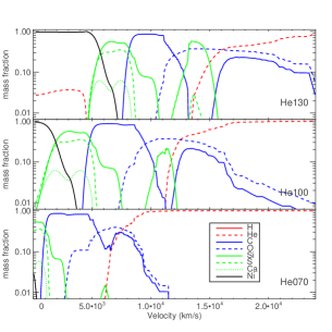
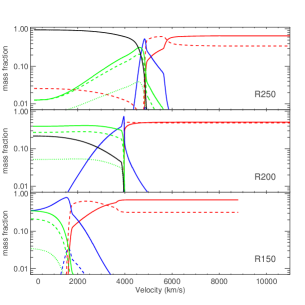
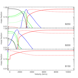
Figure 2.— Ejecta abundance structures of three of the PI SN models in the homologous expansion phase. An artificial smearing of the compositional interfaces has been applied to mimic multi-dimensional mixing processes.

2.1. Stellar Evolution Models

The electron-positron pair-instability supernova mechanism was originally discussed by Rakavy & Shaviv (1967) and Barkat et al. (1967), and has since been explored with a number of numerical and analytic models (see Heger & Woosley, 2002, and references therein). Most recently, Heger & Woosley (2002) [hereafter HW02] explored the explosion of non-rotating bare helium cores with a range of masses from 64 to 133 $\mathrm{M}_{\odot}$. A subset of these models, with masses 70 - 130 $\mathrm{M}_{\odot}$ (in steps of 10 $\mathrm{M}_{\odot}$) will be examined here.

Models of bare helium cores, though computationally expedient, likely do not fully represent the class of PI SNe, as not all stars will have lost their hydrogen envelopes to mass loss or binary mass exchange just prior to exploding. We therefore evolved a new set of models especially for this study of the breakout transients, light curves, and spectra. They consist of five models each of “hydrogenic” (i.e., possessing hydrogen) stars in the main sequence mass range 150 to 250 $\mathrm{M}_{\odot}$, with initial metallicities of 0 and 10^-4 times solar. The surface zoning of these models was chosen much finer than those of HW02 in order to facilitate calculation of the shock breakout emission. In addition, one helium core of mass 100 $\mathrm{M}_{\odot}$ was calculated with three orders of magnitude finer surface zoning (to 10^-8 $\mathrm{M}_{\odot}$) than in HW02. All models were calculated using the Kepler code and the physics discussed in HW02 and Woosley et al. (2002). One difference with the previous studies is that mass loss was included in the hydrogenic stars with non-zero metallicity; however, the mass lost was both small and very uncertain.

Properties of all presupernova stars and their explosions are given in Table 1. The major distinction between the zero metallicity and 10^-4 solar metallicity presupernova stars was that the former died as compact blue supergiants (BSG) while the latter were red supergiants (RSG) with radii 10 to 50 times larger. To some extent, this difference also relies on a particular choice of uncertain parameters – in particular primary nitrogen production and mixing – so not too much weight should be placed on the metallicity of the model. The production of primary nitrogen was, by design, minimal in all models. In the zero metallicity series, especially the higher mass ones, this required reducing semi-convection by a factor of 10 compared with its usual setting in Kepler and turning off overshoot mixing. Unless this was done, only the 150 $\mathrm{M}_{\odot}$ model ended up as a blue supergiant while the other four were red owing to primary nitrogen production.

For the 150, 175, and 200 $\mathrm{M}_{\odot}$ stars with 10^-4 solar metallicity, both semi-convection and overshoot mixing had their nominal settings, but red supergiants resulted without primary nitrogen production. The 225 and 250 $\mathrm{M}_{\odot}$ stars with 10^-4 solar metallicity used the reduced mixing - again to avoid large ¹⁴N production - but also ended up as red supergiants. Since even a moderate amount of rotation would lead to some mixing between the helium core and hydrogen envelope in the zero metal stars, and since the nominal semi-convection and overshoot parameters also lead to primary nitrogen production, it is likely that a fraction, perhaps all, of the zero metallicity pair instability stars also die as red supergiants. This would imply that blue supergiants are a rare population of supernova progenitors for such massive stars even at ultra-low metallicity. Our goal here though was to prepare a set of blue and red supergiant progenitors with a range of masses to explore how the observable properties of the explosion may depend on the structure of the hydrogen envelope.

2.2. Explosion

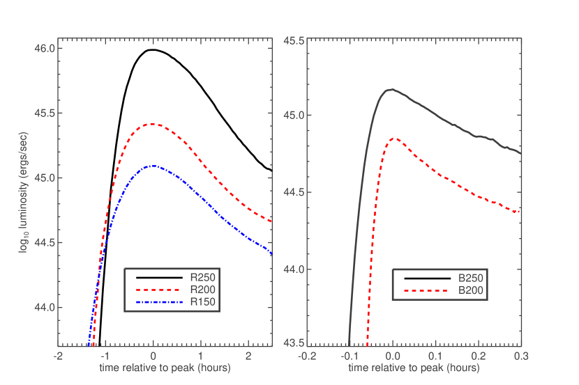
Figure 3.— Calculated bolometric light curves of the shock breakout transient from pair-instability explosions of massive red-supergiant (left) and blue-supergiant (right) stars. The duration of the burst, determined by the light crossing time, is significantly longer for the more extended red supergiant models.

The pair instability is triggered in helium cores above about 40 $\mathrm{M}_{\odot}$ once the temperature in the stellar core exceeds $\sim 10^{9}$ K, i.e., after helium burning and during carbon ignition. The creation of $e^{+}/e^{-}$ pairs in the core then softens the equation of state to below $\gamma<4/3$ leading to instability and collapse. For helium cores below about 135 $\mathrm{M}_{\odot}$ the collapse is eventually reversed by explosive nuclear burning, first of oxygen and, for more massive cores, silicon. Non-rotating helium cores more massive than 133 $\mathrm{M}_{\odot}$ experience a photo-disintegration instability after silicon burning and collapse directly to a black hole (HW02). Between 40 and 60 $\mathrm{M}_{\odot}$, the pair instability in bare helium cores leads to multiple violent mass ejections, but does not disrupt the entire star on the first try (Woosley et al., 2007). Between 60 and 133 $\mathrm{M}_{\odot}$, helium stars collapse to increasing central temperature and density, explode with greater violence, and produce more heavier elements, especially ${}^{56}\mathrm{Ni}$ (see Table 1).

Most of the helium core explosions studied here were taken from the survey by HW02, but the 100 $\mathrm{M}_{\odot}$ model was recalculated with finer surface zoning. A possible point of confusion is whether shocks ever form in these sorts of helium stars or whether, given their small radius, the surface remains in sonic communication with the center throughout the collapse and initial expansion. We find that for the 100 $\mathrm{M}_{\odot}$ model the outer layers do not participate in the collapse and, at about 2 seconds after maximum compression, a very strong shock forms initially about 2 $\mathrm{M}_{\odot}$ beneath the surface at a radius of $8\times 10^{9}$ cm. Due to the large explosion energy and acceleration in the steep density gradient, material in the shock reached a speed of about one-third the speed of light before erupting through the photosphere.

The explosions of the hydrogenic stars had characteristics, including kinetic energy and nucleosynthesis, approximately set by the mass of their helium cores (Table  1). There were, however, some important differences. For the helium stars the mass was set at the beginning of the calculation and held fixed, while in the hydrogenic stars the helium core grew significantly after central hydrogen depletion owing to hydrogen shell burning. In some cases it also shrank due to convective dredge up. At death the helium core thus had a different composition and entropy than a corresponding helium star evolved at constant mass.

An even more significant difference of the hydrogenic stars is that their exploding helium cores encounter the lower density hydrogen envelope and interact with it hydrodynamically. This has several important consequences. First, the expansion of the helium core is slowed, which produces Rayleigh-Taylor instabilities and mixing. Up until this point, the explosion had been determined by simple physics and (assuming no rotation) well represented by a spherical one-dimensional calculation. While the mixing can be calculated in a multi-dimensional code (e.g., Joggerst et al., 2009b), it has not been yet and is parametrized here as in Kasen & Woosley (2009). Except for two models that experienced significant fallback (see below), the mixing has no effect on the nucleosynthesis or energetics and does not affect the breakout emission. However, the late time spectra may be somewhat sensitive to mixing. Figures 1 and 2 plot the final density and mixed compositional structures for a few representative models.

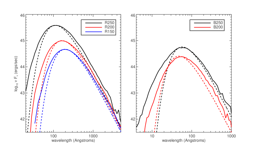
Figure 4.— Synthetic spectra of the shock breakout transients averaged over the burst peak. The time-averaged spectra are the convolution of several blackbodies at different temperatures, and so are broader than a single blackbody function peaking at the same wavelength (dashed lines). Due to the low thermalization opacity, the color temperature is greater than the photospheric temperature by a factor of $2-3$.

In some cases, the deceleration of the helium core by the envelope is so severe that the star doesn’t completely explode. This is particularly true for the blue supergiant models. As pointed out by Chevalier (1989) and explored by Zhang et al. (2008) and Joggerst et al. (2009a), braking and fall back occur to a greater extent in more compact stars. The helium core encounters its own mass earlier and the reverse shock returns to the center when the density is still high. In our case, this resulted in models B150 and B175 failing to eject anything other than their hydrogen envelope. Of course the story does not end there – these bound helium cores oscillate awhile, settle down and evolve again. Given their residual helium masses, models B150 and B175 will probably become pair instability supernovae again and disrupt entirely on the second try. They thus represent an extension to higher masses of the pulsational pair instability supernovae studied by Woosley et al. (2007). Depending upon the timing, the second mass ejection may produce an extremely bright supernova as the very energetic second supernova plows into the ejecta of the first. This future evolution is beyond the scope of the present paper, but the evolution and explosion of blue supergiants with ZAMS masses of 100 - 200 $\mathrm{M}_{\odot}$ is clearly an area worth further study.

3. Observable Properties

3.1. Shock Breakout

In the hydrogenic models, the expansion of the exploded helium core into the hydrogen envelope drives a radiation dominated shock. When this shock approaches the surface of the star, the postshock radiation can escape in a luminous x-ray/UV burst (Klein & Chevalier, 1978; Ensman & Burrows, 1992; Matzner & McKee, 1999). This event occurs at a distance $\Delta R$ from the stellar surface such that the diffusion time from the shock front ($t_{d}\sim\tau\Delta R/c$) is comparable to the dynamical time for the shock to travel the same distance ($t_{e}\sim\Delta R/v_{\rm s}$). This implies an optical depth $\tau\approx c/v_{\rm s}$ at breakout. The shock velocity $v_{\rm s}$ scales with $(E/M)^{1/2}$ and for pair SNe is of order $3\times 10^{3}-10^{4}$ $\mathrm{km~{}s}^{-1}$, similar to that of ordinary core collapse supernovae. Shock breakout thus occurs at optical depths of $\tau_{b}\approx 30-100$.

The surface layers of PI SNe progenitors are difficult to model; a proper representation of the atmospheric structure would require a detailed radiation transport within the stellar evolution code and possibly the inclusion of 3-D effects. The limitations of the 1-D stellar evolution models thus introduce some uncertainty into the breakout predictions. While the current models were much more finely zoned than previous calculations, they still did not fully resolve the optically thin layers of the star. They did, however, determine the slope of the steep density profile at the surface, out to an optical depth of a few. To extend the profile into the optically thin region, we fit a power law to the outermost zones and linearly interpolated and extrapolated the density structure. The re-zoned model had 100 zones within the region $\tau<\tau_{b}$, and extended to a minimum $\tau$ of $10^{-2}$.

We followed the supernova explosion using the Kepler code until the shock front began to approach the stellar surface ($\tau\approx 10^{5}$). The model structure was then mapped into a modified version of the SEDONA transport code (Kasen et al., 2006) which coupled multi-wavelength radiation transport to a staggered mesh 1-D spherical Lagrangian hydrodynamics solver. A standard artificial viscosity prescription was included to damp oscillations behind the shock front. We followed the radiation transport using implicit Monte Carlo methods (Fleck & Cummings, 1971) coupled to the hydrodynamics in an operator split way. The transport was treated in a mixed-frame formalism, in which photon packets were propagated in the inertial frame, but the opacities and emissivities were computed in the comoving frame, and the proper Lorentz transformations were applied to move between the frames. The radiation energy and momentum deposition terms in the hydro equations were estimated by tallying the energy and direction of packets moving through each zone. Further details of the numerical methods in the context of shock breakout will be given in a separate publication Kasen & Woosley (2011).

Table 2Shock Breakout Transients

name	$L_{\rm peak}$ (${\rm ergs~{}s}^{-1}$)	$\Delta t_{h}$	$T_{\rm eff}(10^{5})$	$T_{\rm col}(10^{5})$	$\lambda_{\rm p}$	$E_{\rm p}$	$E_{\rm tot}$	$E_{>L_{\alpha}}$
R250	9.6$\times 10^{45}$	5858	1.3	3.5	82.5	0.15	5.9$\times 10^{49}$	2.2$\times 10^{47}$
R200	2.6$\times 10^{45}$	6422	1.0	2.2	130.5	0.09	1.8$\times 10^{49}$	1.6$\times 10^{47}$
R150	1.2$\times 10^{45}$	7051	0.9	1.7	168.5	0.07	9.3$\times 10^{48}$	1.3$\times 10^{47}$
B250	1.4$\times 10^{45}$	966	3.3	6.3	45.5	0.27	1.3$\times 10^{48}$	6.5$\times 10^{44}$
B200	6.7$\times 10^{44}$	714	3.9	7.7	37.5	0.33	5.8$\times 10^{47}$	1.9$\times 10^{44}$

The opacity and emissivity of the models were discretized into 25000 wavelength bins covering the range $\lambda=0.1-25000$ Å, while the output spectra were binned to a coarser resolution to improve the photon statistics. The dominant opacity in the supernova shock is electron scattering, while free-free is the most important absorptive opacity. Because the current models had zero or very low metallicity, we ignored bound-free and line opacity. At wavelengths near the blackbody peak, the ratio of free-free opacity to total opacity is typically small $\epsilon_{a}\lesssim 10^{-4}$. In the postshock region, Compton up-scattering may then become an important means of energy exchange between matter and radiation (Weaver, 1976). On average, the fractional change of a photon’s energy in a single Compton scattering is $\epsilon_{c}=4kT/m_{e}c^{2}$, which gives an effective $\epsilon_{c}=6\times 10^{-5}$ at $T=10^{5}$ K. Comptonization will significantly alter the radiation spectrum after scattering through an optical depth $\tau_{c}\gtrsim\epsilon_{c}^{-1/2}$ which, for higher temperatures, may be less than the thermalization depth to free-free opacity $\tau_{a}=\epsilon_{a}^{-1/2}$. In our calculations, we therefore approximated the Compton effects by taking a fraction $\epsilon_{c}$ of the Thomson opacity to be thermalizing. This grey absorptive component was added to the wavelength dependent free-free opacity. Clearly a direct treatment of inverse Compton scattering is needed to more accurately predict the spectrum of the breakout burst; nevertheless, our treatment of the full non-grey radiation transport offers some advance over previous numerical calculations.

Once a shock front reaches the steep outer layers of the star, it accelerates down the steep density gradient. For model R250, the shock velocity reaches $v_{s}\approx 1.5\times 10^{4}$ $\mathrm{km~{}s}^{-1}$ around breakout. The temperature of the post-shocked gas is determined by the jump conditions $aT_{s}^{4}/3=\rho_{0}v_{\rm s}^{2}/(\gamma+1)$, where $\rho_{0}$ is the density of the pre-shocked material and $\gamma=4/3$ is the adiabatic index for a radiation dominated gas. Near the surface, the RSG models had densities of $\rho_{0}\sim 10^{-11}$ ${\rm g~{}cm}^{-3}$ which gave typical postshock temperatures of $T_{s}\approx 5\times 10^{5}$ K. The BSG models, being more compact, had higher densities at the surface and hotter temperatures, $T_{s}\approx 10^{6}$ K.

Figure 3 plots the calculated bolometric light curves of the breakout transients. The key observable properties are listed in Table 2. These calculations included the proper light travel time effects, which primarily determined the duration of the observed burst, $\Delta t\approx R_{0}/c$. The RSG models lasted 1 to 2 hours, and reached peak luminosities of $L_{\rm peak}=10^{45}-10^{46}$ ${\rm ergs~{}s}^{-1}$. The BSG models, being more compact, had briefer transients lasting $0.1$ hours, with somewhat lower peak luminosities, $L_{\rm peak}\approx 10^{44}$ ergs/sec. These values can be compared to the breakout in an ordinary Type IIP supernova explosion: $L_{\rm peak}=5\times 10^{44}$ ${\rm ergs~{}s}^{-1}$, $\Delta T=0.5$ hours. As it turns out, the shock velocities and post-shock energy densities of PI SNe are comparable to that of Type IIP supernovae, but the breakout emission can be significantly brighter due to the larger stellar radii.

Figure 4 shows synthetic spectra of the bursts, averaged over the peak of the breakout light curve. The RSG spectra peak at wavelengths $\lambda_{p}=80-170$ Å ($\sim 0.07-0.15$ keV), while the BSG spectra peak near $37-45~{}\AA$ ($\sim 0.3$ keV). These peak wavelengths are comparable to that of ordinary Type IIP breakout ($\lambda_{p}\approx 100$ Å). The spectra are reasonably approximated by a blackbody, but with excess emission at both high and low frequencies. This is because the time-averaged spectra represent a convolution of several blackbodies at different temperatures.

Because the opacity in the atmosphere is strongly scattering dominated, radiation is thermalized at optical depths $\tau\approx\epsilon_{a}^{-1/2}$ well below the photosphere. The emergent spectrum is thus characterized by the higher temperature of these deeper layers. Defining the color temperature $T_{\rm col}$ of the mean spectrum as the temperature of a blackbody peaking at the same wavelength, we find that the observed $T_{\rm col}$ is a typically a factor 2-3 times higher than the effective temperature at the photosphere (Table 2). A similar effect was noted by Ensman & Burrows (1992) for models of SN 1987A. In addition, recent analytic work by Katz et al. (2010) has shown that when the shock velocity is relatively high, $\gtrsim 0.1c$ (and when the thermalization by Compton scattering is treated properly) non-equilibrium effects may lead to a significantly harder non-thermal component in the spectrum. In the BSG models, the shock velocities do in fact reach $\sim 0.1c$ and such a non-thermal component could modify the predicted spectra shown here. The the RSG models, on the other hand, have lower shock velocities and are likely not strongly affected.

Following shock breakout, radiation continues to diffuse out of the expanding, cooling ejecta. This leads to a longer lasting emission that may be visible at optical wavelengths for several weeks. Such an initial thermal component to the light curves is discussed in the following section. The extreme luminosity of the breakout bursts themselves, and their short durations, make them appealing transient to search for in high-redshift surveys. We consider their detectability in Section 4.

3.2. Light Curves

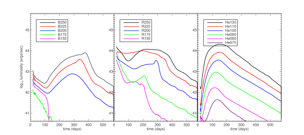
Figure 5.— Bolometric light curves of the full set of models representing the explosion of blue supergiant stars (left panel), red supergiant stars (middle panel) and bare helium cores (right panel). The more massive stars have brighter and longer lasting light curves.

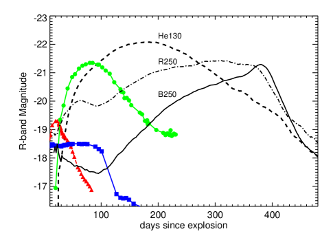
Figure 6.— Synthetic R-band light curves (at $z=0$) of bright PI SN models – R250 (dashed-dot), B250 (solid), and He130 (dashed) – compared to observations of a normal Type Ia supernova SN 2001el (red triangles, Krisciunas et al., 2003) a normal Type IIP supernova SN 1999em (blue squares, Leonard et al., 2002) and the over-luminous core-collapse event SN 2006gy (green circles, Smith et al., 2006).

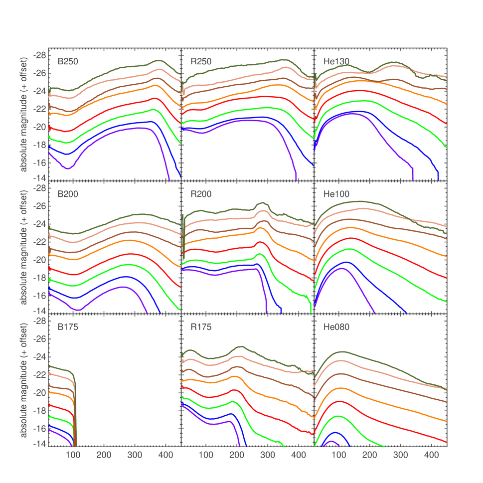
Figure 7.— Broadband light curves of PI SN models. The light curves displayed in each panel are, from bottom to top, UBVRIJHJK. The y-axis corresponds to the B-band light curve, while the other light curves are offset by 1 magnitude from the one above or below.

Following shock breakout, the luminosity of PI SNe can be powered by three different sources: (i) The diffusion of thermal energy deposited by the shock; (ii) the energy from the radioactive decay of synthesized ${}^{56}\mathrm{Ni}$; or (iii) the interaction of the ejecta with a dense surrounding medium. The internal energy suffers adiabatic losses on the expansion timescale $t_{ex}=R_{0}/v$, so source (i) will be most significant for stars with large initial radius $R_{0}$. Interaction has not been included in the models discussed here, but as already mentioned, can be very significant for stars which undergo pulsations before exploding completely.

We calculated light curves of the explosion models using the SEDONA code (Kasen et al., 2006). The initial density, composition, and temperature structures were taken from the Kepler calculations extended into the nearly homologous expansion phase ($\sim 10$ days after explosion). The energy deposition from ${}^{56}\mathrm{Ni}$ decay was followed using a multi-wavelength transport scheme treating the emission, propagation, and absorption of gamma-rays. For the optical radiation transport, the opacities used included electron-scattering, bound-free, free-free, and the aggregate effect of millions of Doppler broadened line transitions treated in the expansion opacity formalism (Eastman & Pinto, 1993). Atomic level populations were calculated assuming local thermodynamic equilibrium, typically a reasonable approximation for supernovae in the photospheric phase.

The resulting model light curves (Figure 5) span a wide range of luminosities and durations. The more massive explosions are bright for over 300 days, with luminosities exceeding $10^{44}$ ergs/sec. The long duration reflects the timescale for photons to diffuse through the optically thick supernova ejecta. In a homologously expanding medium, the effective diffusion time scales as $t_{d}\sim\kappa^{1/2}M_{\rm ej}^{3/4}E^{-1/4}$, where $\kappa$ is the effective mean opacity (Arnett, 1980). Model He130, for example, is nearly 100 times as massive and energetic as a SN Ia, and thus has a light curve $\sim 10$ times as broad. The slow release of energy moderates the emergent luminosity, so that despite making over 60 times as much ${}^{56}\mathrm{Ni}$ as a typical SNe Ia, model He130 is only $\sim 10$ times brighter than one at peak.

The morphology of the model light curves depends on the envelope of the progenitor star. The RSG models resemble Type II plateau supernovae (SNe IIP) light curves, though with luminosities and durations $\sim 3$ times greater. The initial luminosity is powered by the thermal energy in the extended hydrogen envelope. Over time, as the ejecta cool, a hydrogen recombination front propagates inward in mass coordinates, which increases the ejecta transparency due to the elimination of electron scattering opacity. This effect regulates the release of the thermal energy (Grasberg & Nadezhin, 1976; Popov, 1993; Kasen & Woosley, 2009). In the inner regions, heating from radioactive decay delays recombination and causes the light curve to rise to a peak at around $200-300$ days. Eventually, the transparency wave reaches the base of the hydrogen envelope, after which recombination proceeds much more rapidly through the heavier element core. After a rapid release of the remaining internal energy, the light curve drops off sharply and follows directly the radioactive energy deposition rate.

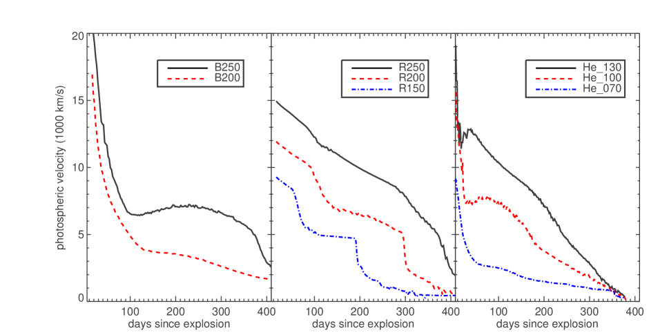
Figure 8.— Time evolution of the velocity measured at the electron scattering photosphere for several PI SN models. In the BSG and helium core models, the photosphere initially recedes quickly as the outer layers recombine and become transparent. The rise in photospheric velocity seen in some models reflects the outward diffusion of radioactive energy which may heat and reionize the external layers.

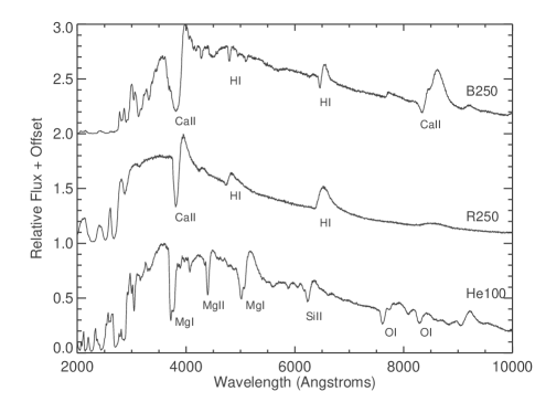
Figure 9.— Spectra of select models at the peak of the light curve. The important line absorption features are marked.

The light curves of the BSG models have a dimmer initial thermal component, due to the relatively smaller radii of the progenitors. In this respect they resemble scaled up versions of SN 1987A. In models B200, B225, and B250, the light curves rise to a bright ${}^{56}\mathrm{Ni}$ powered peak at $\sim 300$ days after explosion. The less massive events (B150 and B175), which failed to eject any ${}^{56}\mathrm{Ni}$, only show the initial thermal light curve component lasting $\sim 150$ days, and more closely resemble typical SNe IIP.

The helium core PI SNe models, being the most compact progenitors, lack a conspicuous thermal light curve component altogether. The lower total mass leads to relatively briefer light curves, peaking around 150 days after explosion. Model He130 ($\sim 40$ $\mathrm{M}_{\odot}$ of ${}^{56}\mathrm{Ni}$) reaches an exceptional peak brightness of $2\times 10^{44}$ ${\rm ergs~{}s}^{-1}$ at around 180 days. Model He70, on the other hand, proves that despite being massive and energetic, not all PI SNe are bright. This explosion produced only $0.02$ $\mathrm{M}_{\odot}$ of ${}^{56}\mathrm{Ni}$ and the light curve reached only $3\times 10^{41}$ ergs/sec, rather sub-luminous for a supernova.

Figure 6 compares the synthetic R-band light curves of representative PI SN models with observations of a typical Type Ia supernova (SN 2001el, Krisciunas et al., 2003), a typical Type IIP supernova (SN 1999em, Leonard et al., 2002), and SN 2006gy, one of the most the luminous core-collapse SNe discovered (Smith et al., 2006). The later has been suggested to be a pair instability supernovae, however the predicted model light curve durations are seen to be too long even for this event by a factor of several. Another possibility is that SN 2006gy was an example of a pulsational-pair instability supernova (Woosley et al., 2007).

Figure 7 shows the multi-color optical and near-infrared light curves for the models. At bluer wavelengths, the light curves generally peak earlier and decline more rapidly after peak. This reflects the progressive shift of the spectral energy distribution to the red over time. This shift is due not only the decrease in effective temperature, but also to the increase in line opacity from iron group elements of lower ionization stages (Fe II and Co II), which blankets the bluer wavelengths.

The brightest helium core models such as He130 display a pronounced secondary maximum in the infrared light curves. This feature is similar to what is observed in Type Ia supernovae and the physical explanation is essentially the same (Kasen, 2006). When the temperature in the ejecta drops below $\sim 7000$ K, doubly ionized iron group elements begin to recombine. As the infrared line emissivity is much greater for singly ionized species (Fe II and Co II) the flux can be more efficiently redistributed from bluer to redder wavelengths, leading to an increase in the infrared luminosity. The secondary maximum is therefore more prominent in models with large abundances of iron group elements. Detection of a secondary maximum in an observed supernova would provide strong evidence that the explosion did indeed synthesize large amounts of ${}^{56}\mathrm{Ni}$. The lack of a secondary maximum does not necessarily rule out the presence of substantial ${}^{56}\mathrm{Ni}$, as strong radial mixing of the nickel can sometimes smear out the two bumps (Kasen, 2006).

3.3. Spectra

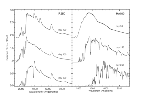
Figure 10.— Spectral evolution of model R250 (left panel) and model He100 (right panel). Over time, additional line features appears as the photosphere recedes into layers of burned material.

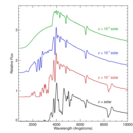
Figure 11.— The day 100 spectrum of model R150 shown for different values of metallicity in the hydrogen envelope, from top to bottom $Z=10^{-6},10^{-4},10^{-2},$ and $1$ times solar. The metallicity can be probed observationally by examining metal line absorption features or the flux in the ultra-violet.

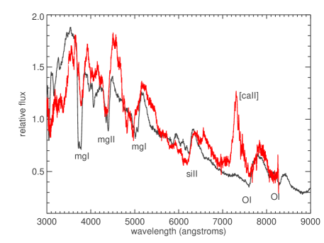
Figure 12.— The spectrum, observed near peak, of SN 2007bi (red line Gal-Yam et al., 2009) compared to the synthetic spectrum of our model He100 at 100 days after explosion (black line). Line identifications for the model are marked. Most of the major observed line features are reproduced by the model, except for the forbidden Ca II line emission at 7300 Å which is the result of non-equilibrium effects not included in the calculations.

The spectra of the PI SN models (Figures 9 and 10) resemble those of ordinary SNe, with P-Cygni line profiles superimposed on a pseudo-blackbody continuum. Because of the low abundance of metals in unburned ejecta, many of the familiar line features are weak or missing in the early time spectra. For example, at maximum light models R250 and B250 show only features from the hydrogen Balmer lines and calcium in their spectrum. However, at later times, when the photosphere has receded into layers of burned material, other line features appear.

The maximum light spectrum of the bare helium core model He100 is dominated by lines from freshly synthesized intermediate mass elements, and resembles a Type Ic SN with lines due to Mg I, Mg II, Si II, Ca II and O I. After peak, the spectrum shows more features from the iron group elements in the ${}^{56}\mathrm{Ni}$-rich core. Helium lines are not present at any epoch, as the envelope temperatures are too low to thermally excite the lower atomic levels of the optical transitions. However, if ${}^{56}\mathrm{Ni}$ is mixed out into the helium rich layers, non-thermal excitation by radioactive decay products could generate significant helium line opacity (Lucy, 1991).

Although PI SNe are highly energetic events, their large ejected masses imply only moderate characteristic velocities: $v\sim(2E_{\rm K}/M_{\rm ej})^{1/2}\sim 5000$ $\mathrm{km~{}s}^{-1}$, about half that typical of SNe Ia and several times less then the broad lined Type Ic SNe that have been associated with gamma-ray bursts (Galama et al., 1998). Figure 8 show the time evolution of the velocity measured at the electron scattering photosphere. In the BSG and helium core models, the photosphere initially resides in the outer, high velocity layers of ejecta, but recedes quickly as these layers recombine and become transparent. Eventually, the photosphere settles in the inner regions of burned material, where radioactive energy deposition maintains the ionization state. Interestingly, the photospheric velocity in model B250 in fact increases for some time period as the radioactive energy diffuses outward and reionizes the hydrogen envelope. In contrast, the decline in photospheric velocity in the RSG models is gradual until the recombination front reaches the base of the hydrogen envelope, after which it drops off sharply.

Certain features in the spectra of PI SNe could, if observed, offer direct confirmation that the progenitor star was of low metallicity. The metallicity has two principle spectroscopic effects (Figure 11). First, for metallicities $Z\geq 10^{-4}$, some absorption lines from intermediate mass elements are noticeable, for example those of Ca II H&K (near 3800 Å) and the IR triplet (near 8300 Å). Second, higher metallicity leads to a significant reduction in the ultraviolet (UV) flux, due to the iron group line blanketing at bluer wavelengths. Similar metallicity effects have been noted in the spectral modeling of Type IIP SNe (Baron et al., 2003; Dessart & Hillier, 2005) Spectroscopic or rest frame UV observations of PI SNe may, together with modeling, constrain the metallicity of the progenitor star. This assumes, of course, that the supernova has been observed early enough that we are seeing layers of ejecta unaffected by the explosive nucleosynthesis.

To draw some comparison to observations, Figure 12 shows the near maximum light spectrum of one model, He100, compared to the most promising candidate to date for an observed pair supernova, SN 2007bi. Gal-Yam et al. (2009) has previously shown that the light curve of this supernova is a good match to model He100. On the whole, the correspondence of the spectra is also rather good, especially considering that the model has not been tuned to match the data. Most of the major line features are reproduced, in particular the unusually prominent Mg I and Mg II lines. The ejecta velocities (as evidenced by the blueshift of the absorption features) are also roughly in agreement. The model fails to reproduce the forbidden Ca II line emission at 7300 Å, but this feature results from non-equilibrium effects which are not included in our calculations.

4. Detectability

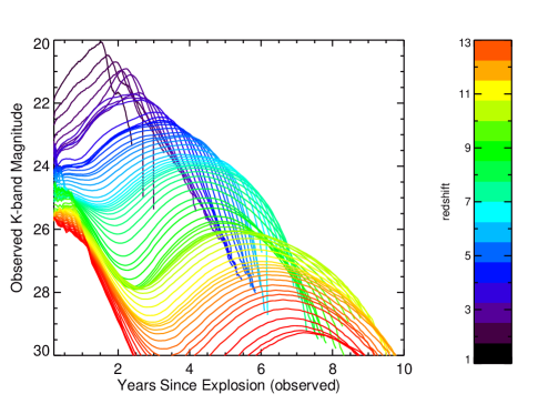
Figure 13.— Observer frame K-band light curve of model R250 as a function of redshift. The effects of cosmological redshift, dimming, and time-dilation have all been included. For $z>7$, one observes in the rest-frame UV, and the initial thermal component of the light curve is brighter than the later radioactively powered peak.

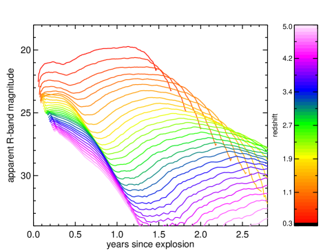
Figure 14.— Observer frame R-band light curve of model R250 as a function of redshift. The effects of cosmological redshift, dimming, and time-dilation have all been included.

Some PI SNe should be observable out to large distances, but the effects of cosmological redshift and time-dilation effects will significantly affect the shape and luminosity of the observed light curve. Figures 13 and 14 demonstrate these effects for model R250 in the K- and R-bands, respectively. The radioactively powered optical emission, which lasts for hundreds of days, emits very little flux at rest wavelengths $\lambda<2000$ Å. Thus, to follow objects at $z\geq 5$ it is best to observe at infrared wavelengths. Alternatively, one could search for the brief and very blue emission from shock breakout.

In Figures 15 and 16 we plot the observer frame R- and K-band peak magnitudes of several PI SN light curves (starting $t>10$ days after explosion in the rest-fame) as a function of redshift. Future R-band surveys, such as with the Large Synoptic Survey Telescope, will routinely reach limiting magnitudes of $M_{R}\sim 24.5$, which would detect or place constraints on the brightest PI SNe out to redshift of $z\sim 2$. Deeper searches ($M_{R}\sim 28$) would reach redshifts $z\sim 5$, while a similar K-band search would probe redshifts of $z\sim 10$ and beyond. Space based observations at wavelengths longer than K-band could potentially see to even greater distances. The long duration of the PI SN light curves – greatly prolonged by the $(1+z)$ cosmological time dilution factor – poses a challenge for detecting them as transients. At $z\sim 7$ the light curve of a PI SN can last 1 to 5 years in the observers frame (Figures 13 and 14). Deep exposures over long time baselines would be needed to discover and follow such an event.

An alternative way of discovering PI SNe would be to search for the short-lived shock breakout transient. At $z=1$, the observed burst would last a few hours, and at $z=10$ about a day. The spectrum, which peaks in the rest-frame at $\lambda\approx 80-170$ Å, would be seen on the Rayleigh-Jeans tail. Unfortunately, neutral hydrogen along the line of sight likely absorbs all radiation shortwards of the Lyman alpha line at 1215 Å, which is the bulk of the radiation emitted in shock breakout. However, the radiation at longer wavelengths can be significant and may still be visible.

Figure 17 plots the observed AB magnitudes (in different wavelength bands) of the RSG models at the peak of the bolometric breakout light curve. At redshifts $z>3$ the curves flatten out as flux is redshifted into the observed band and compensates for the greater distance. An all sky optical survey like LSST which reached magnitude $R\approx 24.5$ per image could potentially catch shock breakout to redshifts of $z\approx 1$. In principle, deeper optical imaging in select fields could detect breakout to much higher redshift, but in practice, the Lyman limit restricts the optical detectability to $z\sim 6$.

Near-infrared surveys could avoid the problem of hydrogen absorption. A facility like JWST with $\lesssim 10$ nJ ($M_{ab}\sim 29$) sensitivity in the wavelength region $2-5\mu$ has the capability of detecting shock breakout out at redshifts of $z\approx 10-20$. However, the small field of view of JWST, combined with the expected low rates of PI SNe, suggest that it will be unlikely to discover a PI SNe in this manner. A wide-field imager with infrared capabilities (e.g., WFIRST or EUCLID) may fare better for discovering shock breakout at the highest redshifts.

The rates of PI SNe, in either the nearby or distance universe, are very uncertain. Scannapieco et al. (2005) (see also Scannapieco et al. (2003)) provided one estimate of the rate as of one PI SN per 1000 solar masses of metal free stars, with the metal free stars themselves forming, at all redshifts, at only 1% of the total star formation rate. Observationally, the detection of at least on promising candidate pair SN (SN 2007bi) suggests a rate in the local universe of $\lesssim 10^{-4}$ of the core collapse rate (Quimby et al., 2009; Gal-Yam et al., 2009). More detailed investigation of the PI SN rate will be considered elsewhere (Pan et al., in prep) but in any case it should be kept in mind that PI SNe are rare compared to other supernovae, and will therefore be difficult to discover in bulk.

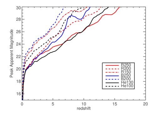
Figure 15.— Detectability of pair instability supernovae light curves. The figure plots the observer-frame peak K-band magnitude of several models as a function of redshift.

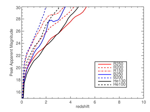
Figure 16.— Same as Figure 15, but for the R-band.

5. Summary and Conclusions

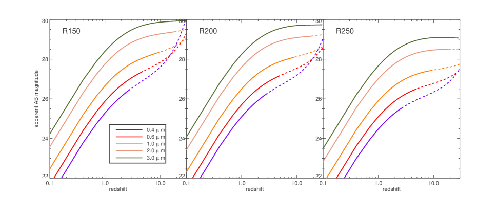
Figure 17.— Detectability of the shock breakout transient from pair instability supernovae as a function of redshift. The figure plots the observed AB magnitude (for different wavelength bands) of three red-supergiant models at the peak of the bolometric breakout light curve. (Note an AB magnitude of 28.9 corresponds to $10~{}$nJ.) Solid lines denote the redshift range for which the rest frame flux is redder than $1216~{}\AA$ (the Lyman alpha line); at higher redshifts, the flux is likely absorbed by intervening neutral hydrogen (dashed lines). The breakout transients of the blue supergiant models will be significantly dimmer than the models shown here, as the luminosity is lower and the spectrum peaks at much lower wavelengths.

We have surveyed the spectra, multi-color light curves, and shock breakout transients of pair instability supernova models throughout the mass range in which the star suffers complete disruption. Three varieties of progenitor stars were explored: i) helium cores that may have resulted when very massive stars either lost their envelopes to some sort of non-radiative mass loss (as in Eta Carina) or to a binary companion; ii) blue supergiants still retaining most of their hydrogen envelope; and iii) red supergiants with enormous radii. The frequency and distribution with mass and metallicity of ii) and iii) depends on uncertain parameters of semiconvection and overshoot; in general it seems that the red supergiants are a more common outcome of the stellar evolution than blue supergiants.

Though PI SNe are often considered to be categorically bright events, in fact it is only the most massive stars ($M>200$ $\mathrm{M}_{\odot}$) that are extraordinary in terms of luminosity. The lower mass objects have peak brightnesses comparable to normal core collapse events $L=10^{42}-10^{43}$ ergs, though the light curves last for much longer. For a sensible initial mass function, it is likely that these dimmer events are actually the more representative PI SNe. An extended light curve, rather than an extreme luminosity, may therefore be the most relevant signature of the pair instability events.

The models illustrate how the different classes of progenitor stars can be distinguished observationally by the light curve morphology. The red supergiant explosions have light curves with long duration plateaus, similar to ordinary Type IIP supernovae but with luminosities and durations $\sim 3$ times greater. The light curves of the blue-supergiant explosions more closely resemble SN 1987A, with a brief initial thermal component and a late, prominent ${}^{56}\mathrm{Ni}$ powered peak. The bare helium core model light curves resemble very long lasting Type Ib/Ic supernovae.

The exploding cores of the more compact blue supergiant progenitors are braked extensively by hydrodynamic interaction with their envelopes. For the lighter stars considered (models B150 and B175) the system failed to completely explode on the first try, and only the outer envelope of the star was ejected. The class of pulsational pair instability may thus have a larger range than stated by Woosley et al. (2007). A secondary explosion of the helium core, and its subsequent collision with the ejected hydrogen envelope, could then lead to an extremely luminous supernova event.

Despite the large explosion energy of PI SNe, the expansion velocities, as measured from the Doppler shift of spectral lines, are rather low $v\approx 5000-10000~{}\mathrm{km~{}s}^{-1}$. The spectra of helium core explosions resemble Type Ic supernovae, and in particular are distinguished by prominent lines of Mg I and Mg II. The spectra of hydrogenic models appear in most respects like ordinary Type II supernovae, however the absence of certain metal line features (e.g., the Ca II IR triplet) and the bright ultraviolet emission (due to the reduced iron group line blanketing) may provide signatures that the stellar envelope was indeed of very low metallicity.

The recently publicized SN 2007bi has been suggested to be the first convincing detection of a PI SN. Gal-Yam et al. (2009) compared the observed light curve of SN 2007bi to the models presented here, and found very good agreement with a helium core explosion of mass 100-110 $\mathrm{M}_{\odot}$. We have shown here that the spectrum of the helium core model is also in reasonable agreement with the observations, and in particular with the presence of strong magnesium lines. SN 2007bi is therefore a compelling candidate for a PI SN, however other possible scenarios have been suggested. Moriya et al. (2010) have shown that the light curve could be explained as well by the core collapse of a massive 43 $\mathrm{M}_{\odot}$ C/O core. Another possibility is that the light curve was powered not by ${}^{56}\mathrm{Ni}$ decay, but by energy injection from a highly magnetized remnant neutron star (a magnetar Kasen and Bildsten, 2010; Woosley, 2010)). The distinguishing feature of the pair SNe model is its exceptionally long rise time, but unfortunately the observations of SN 2007bi lacked data before the peak . At present, one appealing feature of the pair SNe model for SN 2007bi is that it correctly predicts the explosion energy, given the progenitor star mass. In the other models, the energy is a free parameter that must be input by hand to match the observed light curves and spectra.

Other luminous observed supernovae, such as SN 2006gy (Smith et al., 2006), SN 2005ap (Quimby et al., 2007), and SN 2008es (Gezari et al., 2009) have occasionally been suggested to be examples of PI SNe. However, the light curve duration of these events ($\sim 50-100$ days) are simply too short to be explained by the classic ${}^{56}\mathrm{Ni}$ powered pair explosions explored here, which all last of order $\sim 300$ days. The pulsational pair scenario, which occurs for stellar masses just below those considered here, provide a possible explanation for these observations, as does magnetar energy injection.

It is often lamented that pair SNe cannot be discovered as transients at high redshift – their intrinsically slow ($\sim 1$ year) light curve evolution, prolonged by a $(1+z)$ cosmological time dilation, will exceed the lifetime of most observational surveys. Actually, the situation is not all that bad. For example, in our 100 $\mathrm{M}_{\odot}$ helium model the bolometric light curve declines (after peak) at at a rate of about 0.01 mag per day. At a redshift of $z=10$, this results in a $\sim 0.3$ mag variation over an observer frame year. That may be within the sensitivity of future surveys with multi-year baselines. Moreover, we find that the decline is more rapid in the bluer bands (due to the increasing onset of iron group line blanketing at these wavelengths) such that variations in the restframe U- and B-bands are a factor of $2-3$ larger. Even if the temporal variations are too hard to measure, the colors of PI SNe might be distinct enough that one could use them to select candidates for further follow up.

An alternative approach for finding PI SNe would be to look for the brief, but very luminous emission of shock breakout. For the larger red-supergiant explosions, the breakout transients are 20 times as luminous ($L_{\rm peak}\approx 10^{46}~{}{\rm ergs~{}s}^{-1}$) as those of typical Type IIP supernovae, and last about four times as long ($\sim 2$ hours). The emission peaks in the rest-frame far ultraviolet ($\lambda\sim 80-170$ Å). Sensitive surveys in the infrared ($2-5~{}\mu$m) with a high cadence and a wide-field of view could, in principle, detect these transients out to high redshifts. Once detected, the subsequent ${}^{56}\mathrm{Ni}$ powered light curve and spectra could be monitored, with some leisure, for many years to come.

References

- Abel et al. (2000) Abel, T., Bryan, G. L., & Norman, M. L. 2000, ApJ, 540, 39
- Arnett (1980) Arnett, W. D. 1980, ApJ, 237, 541
- Barkat et al. (1967) Barkat, Z., Rakavy, G., & Sack, N. 1967, Physical Review Letters, 18, 379
- Barbary et al. (2009) K. Barbary, et al., ApJ 690, 1358–1362 (2009),
- Baron et al. (2003) Baron, E., Nugent, P. E., Branch, D., Hauschildt, P. H., Turatto, M., & Cappellaro, E. 2003, ApJ, 586, 1199
- Bond et al. (1984) Bond, J. R., Arnett, W. D., & Carr, B. J. 1984, ApJ, 280, 825
- Bromm et al. (1999) Bromm, V., Coppi, P. S., & Larson, R. B. 1999, ApJ, 527, L5
- Chevalier (1989) Chevalier, R. A. 1989, ApJ, 346, 847
- Dessart & Hillier (2005) Dessart, L., & Hillier, D. J. 2005, A&A, 437, 667
- Eastman & Pinto (1993) Eastman, R. G., & Pinto, P. A. 1993, ApJ, 412, 731
- Ensman & Burrows (1992) Ensman, L., & Burrows, A. 1992, ApJ, 393, 742
- Fleck & Cummings (1971) Fleck, J., & Cummings, J. 1971, JQSRT, 8, 313
- Fryer et al. (2010) Fryer, C. L., Whalen, D. J., & Frey, L. 2010, ArXiv e-prints
- Gal-Yam et al. (2009) Gal-Yam, A. et al. 2009, Nature, 462, 624
- Galama et al. (1998) Galama, T. J., et al. 1998, Nature, 395, 670
- Gezari et al. (2009) Gezari, S. et al. 2009, ApJ, 690, 1313
- Grasberg & Nadezhin (1976) Grasberg, E. K., & Nadezhin, D. K. 1976, Ap&SS, 44, 409
- Heger et al. (2003) Heger, A., Fryer, C. L., Woosley, S. E., Langer, N., & Hartmann, D. H. 2003, ApJ, 591, 288
- Heger & Woosley (2002) Heger, A., & Woosley, S. E. 2002, ApJ, 567, 532
- Joggerst et al. (2009a) Joggerst, C. C., Almgren, A., Bell, J., Heger, A., Whalen, D., & Woosley, S. E. 2009a, ArXiv e-prints
- Joggerst et al. (2009b) Joggerst, C. C., Woosley, S. E., & Heger, A. 2009b, ApJ, 693, 1780
- Kasen (2006) Kasen, D. 2006, ApJ, 649, 939
- Kasen et al. (2006) Kasen, D., Thomas, R. C., & Nugent, P. 2006, ApJ, 651, 366
- Kasen & Woosley (2009) Kasen, D., & Woosley, S. E. 2009, ApJ, 703, 2205
- Kasen and Bildsten (2010) D. Kasen, and L. Bildsten, ApJ 717, 245–249 (2010).
- Kasen & Woosley (2011) Kasen, D., & Woosley, S. 2011, in preparation
- Katz et al. (2010) Katz, B., Budnik, R., & Waxman, E. 2010, ApJ, 716, 781
- Klein & Chevalier (1978) Klein, R. I., & Chevalier, R. A. 1978, ApJ, 223, L109
- Knop et al. (1999) Knop, R. et al. 1999, IAU Circ., 7128, 1
- Krisciunas et al. (2003) Krisciunas, K. et al. 2003, AJ, 125, 166
- Leonard et al. (2002) Leonard, D. C. et al. 2002, AJ, 124, 2490
- Lucy (1991) Lucy, L. B. 1991, ApJ, 383, 308
- Matzner & McKee (1999) Matzner, C. D., & McKee, C. F. 1999, ApJ, 510, 379
- Moriya et al. (2010) Moriya, T., Tominaga, N., Tanaka, M., Maeda, K., & Nomoto, K. 2010, ApJ, 717, L83
- Nakamura & Umemura (2001) Nakamura, F., & Umemura, M. 2001, ApJ, 548, 19
- Pan (2008) Pan, T. et al., 2011, in prep
- Popov (1993) Popov, D. V. 1993, ApJ, 414, 712
- Quimby et al. (2007) Quimby, R. M., Aldering, G., Wheeler, J. C., Höflich, P., Akerlof, C. W., & Rykoff, E. S. 2007, ApJ, 668, L99
- Quimby et al. (2009) Quimby, R. M., et al. 2009, arXiv:0910.0059
- Rakavy & Shaviv (1967) Rakavy, G., & Shaviv, G. 1967, ApJ, 148, 803
- Rakavy et al. (1967) Rakavy, G., Shaviv, G., & Zinamon, Z. 1967, ApJ, 150, 131
- Scannapieco et al. (2003) Scannapieco, E., Schneider, R., & Ferrara, A. 2003, ApJ, 589, 35
- Scannapieco et al. (2005) Scannapieco, E., Madau, P., Woosley, S., Heger, A., & Ferrara, A. 2005, ApJ, 633, 1031
- Smith et al. (2006) Smith, N. et al. 2006, ArXiv Astrophysics e-prints
- Smith & McCray (2007) Smith, N., & McCray, R. 2007, ApJ, 671, L17
- Umeda & Nomoto (2002) Umeda, H., & Nomoto, K. 2002, ApJ, 565, 385
- Waldman (2008) Waldman, R. 2008, ApJ, 685, 1103
- Weaver (1976) Weaver, T. A. 1976, ApJS, 32, 233
- Woosley (2010) Woosley, S. E. 2010, ApJ, 719, L204
- Woosley et al. (2007) Woosley, S. E., Blinnikov, S., & Heger, A. 2007, Nature, 450, 390
- Woosley et al. (2002) Woosley, S. E., Heger, A., & Weaver, T. A. 2002, Reviews of Modern Physics, 74, 1015
- Young et al. (2010) Young, D. R. et al. 2010, A&A, 512, A70+
- Zhang et al. (2008) Zhang, W., Woosley, S. E., & Heger, A. 2008, ApJ, 679, 639