1 Introduction
One way of characterizing a distribution of an absolutely continuous random variable X 𝑋 X h 0 subscript ℎ 0 h_{0} X 𝑋 X ϵ > 0 italic-ϵ 0 \epsilon>0 ϵ h 0 ( x ) italic-ϵ subscript ℎ 0 𝑥 \epsilon h_{0}(x) ( x , x + ϵ ] 𝑥 𝑥 italic-ϵ (x,x+\epsilon] x 𝑥 x h 0 subscript ℎ 0 h_{0} x 𝑥 x h 0 ( x ) subscript ℎ 0 𝑥 h_{0}(x) x 𝑥 x x 𝑥 x
It is especially this clear interpretation of these qualitative properties of a hazard rate that makes this function a natural characteristic of a survival distribution. The problem of estimating a hazard rate nonparametrically under qualitative (or shape) restrictions gained attention in the sixties of the previous century (see [ Groeneboom and Jongbloed (2011b) ] [ Proschan and Pyke (1967) ] [ Groeneboom and Jongbloed (2011a) ]
In this paper, we consider the asymptotic distribution theory for two integral-type test statistics for the hypothesis that a hazard rate h 0 subscript ℎ 0 h_{0} [ 0 , a ] 0 𝑎 [0,a] a > 0 𝑎 0 a>0
Based on an i.i.d. sample X 1 , … , X n subscript 𝑋 1 … subscript 𝑋 𝑛
X_{1},\ldots,X_{n} H 0 subscript 𝐻 0 H_{0} H 0 subscript 𝐻 0 H_{0} H 0 subscript 𝐻 0 H_{0}
ℍ n ( x ) = { − log { 1 − 𝔽 n ( x ) } , x ∈ [ 0 , X ( n ) ) , ∞ , x ≥ X ( n ) subscript ℍ 𝑛 𝑥 cases 1 subscript 𝔽 𝑛 𝑥 𝑥 0 subscript 𝑋 𝑛 missing-subexpression 𝑥 subscript 𝑋 𝑛 missing-subexpression {\mathbb{H}}_{n}(x)=\left\{\begin{array}[]{lll}-\log\left\{1-{\mathbb{F}}_{n}(x)\right\},&x\in\left[0,X_{(n)}\right),\\
\infty,&x\geq X_{(n)}\end{array}\right.
where 𝔽 n subscript 𝔽 𝑛 {\mathbb{F}}_{n} X 1 , X 2 , … , X n subscript 𝑋 1 subscript 𝑋 2 … subscript 𝑋 𝑛
X_{1},X_{2},\ldots,X_{n} H 0 subscript 𝐻 0 H_{0} [ 0 , a ] 0 𝑎 [0,a] H ^ n subscript ^ 𝐻 𝑛 \hat{H}_{n} ℍ n subscript ℍ 𝑛 {\mathbb{H}}_{n} [ 0 , a ] 0 𝑎 [0,a]
T n = ∫ [ 0 , a ] { ℍ n ( x − ) − H ^ n ( x ) } 𝑑 𝔽 n ( x ) . subscript 𝑇 𝑛 subscript 0 𝑎 subscript ℍ 𝑛 limit-from 𝑥 subscript ^ 𝐻 𝑛 𝑥 differential-d subscript 𝔽 𝑛 𝑥 T_{n}=\int_{[0,a]}\bigl{\{}{\mathbb{H}}_{n}(x-)-\hat{H}_{n}(x)\bigr{\}}\,d{\mathbb{F}}_{n}(x). (1.1)
Note that this is the empirical L 1 subscript 𝐿 1 L_{1} d 𝔽 n 𝑑 subscript 𝔽 𝑛 d{\mathbb{F}}_{n} T n ≥ 0 subscript 𝑇 𝑛 0 T_{n}\geq 0 H ^ n subscript ^ 𝐻 𝑛 \hat{H}_{n} ℍ n subscript ℍ 𝑛 {\mathbb{H}}_{n} H 0 subscript 𝐻 0 H_{0} [ 0 , a ] 0 𝑎 [0,a] H 0 subscript 𝐻 0 H_{0} H 0 subscript 𝐻 0 H_{0} T n subscript 𝑇 𝑛 T_{n} n → ∞ → 𝑛 n\rightarrow\infty h 0 subscript ℎ 0 h_{0} [ 0 , a ] 0 𝑎 [0,a] ℍ n subscript ℍ 𝑛 {\mathbb{H}}_{n} H 0 subscript 𝐻 0 H_{0} H 0 subscript 𝐻 0 H_{0} H ^ n subscript ^ 𝐻 𝑛 \hat{H}_{n} H 0 subscript 𝐻 0 H_{0} [ 0 , a ] 0 𝑎 [0,a] T n = 0 subscript 𝑇 𝑛 0 T_{n}=0 H ^ n subscript ^ 𝐻 𝑛 \hat{H}_{n} ( x ( i ) , ℍ n ( x ( i ) − ) ) subscript 𝑥 𝑖 subscript ℍ 𝑛 limit-from subscript 𝑥 𝑖 (x_{(i)},{\mathbb{H}}_{n}(x_{(i)}-)) [ 0 , a ] 0 𝑎 [0,a] T n = 0 subscript 𝑇 𝑛 0 T_{n}=0 ℍ n subscript ℍ 𝑛 {\mathbb{H}}_{n} [ 0 , a ] 0 𝑎 [0,a] ℍ n ( x − ) subscript ℍ 𝑛 limit-from 𝑥 {\mathbb{H}}_{n}(x-) ℍ n ( x ) subscript ℍ 𝑛 𝑥 {\mathbb{H}}_{n}(x) 1.1
U n = ∫ [ 0 , a ) { 𝔽 n ( x − ) − F ^ n ( x ) } 𝑑 𝔽 n ( x ) , where F ^ n ( x ) = 1 − exp ( − H ^ n ( x ) ) . formulae-sequence subscript 𝑈 𝑛 subscript 0 𝑎 subscript 𝔽 𝑛 limit-from 𝑥 subscript ^ 𝐹 𝑛 𝑥 differential-d subscript 𝔽 𝑛 𝑥 where subscript ^ 𝐹 𝑛 𝑥 1 subscript ^ 𝐻 𝑛 𝑥 U_{n}=\int_{[0,a)}\bigl{\{}{\mathbb{F}}_{n}(x-)-\hat{F}_{n}(x)\bigr{\}}\,d{\mathbb{F}}_{n}(x),\mbox{ where }\hat{F}_{n}(x)=1-\exp(-\hat{H}_{n}(x)). (1.2)
An advantage of this definition is that U n subscript 𝑈 𝑛 U_{n} ℍ n subscript ℍ 𝑛 {\mathbb{H}}_{n}
The main result of this paper concerns the asymptotic distribution of T n subscript 𝑇 𝑛 T_{n} U n subscript 𝑈 𝑛 U_{n}
n 5 / 6 { T n − E T ~ n } ⟶ 𝒟 N ( 0 , σ H 0 2 ) and n 5 / 6 { U n − E U n } ⟶ 𝒟 N ( 0 , σ F 0 2 ) , superscript ⟶ 𝒟 superscript 𝑛 5 6 subscript 𝑇 𝑛 𝐸 subscript ~ 𝑇 𝑛 𝑁 0 superscript subscript 𝜎 subscript 𝐻 0 2 and superscript 𝑛 5 6 subscript 𝑈 𝑛 𝐸 subscript 𝑈 𝑛 superscript ⟶ 𝒟 𝑁 0 superscript subscript 𝜎 subscript 𝐹 0 2 n^{5/6}\left\{T_{n}-E\tilde{T}_{n}\right\}\stackrel{{\scriptstyle{\cal D}}}{{\longrightarrow}}N\left(0,\sigma_{H_{0}}^{2}\right)\mbox{ and }n^{5/6}\left\{U_{n}-EU_{n}\right\}\stackrel{{\scriptstyle{\cal D}}}{{\longrightarrow}}N\left(0,\sigma_{F_{0}}^{2}\right), (1.3)
where T ~ n subscript ~ 𝑇 𝑛 \tilde{T}_{n} T n subscript 𝑇 𝑛 T_{n} 4.1 4.2 σ H 0 2 superscript subscript 𝜎 subscript 𝐻 0 2 \sigma_{H_{0}}^{2} σ F 0 2 superscript subscript 𝜎 subscript 𝐹 0 2 \sigma_{F_{0}}^{2} f 0 subscript 𝑓 0 f_{0} [ Kulikov and Lopuhaä (2008) ]
The basic idea of the proof is to approximate the integral in the test statistic as sum of increasingly many local integrals, using the crucial localization Lemma 3.4 2 3 T n subscript 𝑇 𝑛 T_{n} F 0 subscript 𝐹 0 F_{0} 𝔽 n subscript 𝔽 𝑛 {\mathbb{F}}_{n} [ Rosenblatt (1956) ] 2 1.3 4 d 𝔽 n 𝑑 subscript 𝔽 𝑛 d{\mathbb{F}}_{n} d F 0 𝑑 subscript 𝐹 0 dF_{0}
2 Asymptotic local problem
Consider the process
x ↦ V ( x ) = W ( x ) + x 2 , x ∈ ℝ formulae-sequence maps-to 𝑥 𝑉 𝑥 𝑊 𝑥 superscript 𝑥 2 𝑥 ℝ x\mapsto V(x)=W(x)+x^{2},\,x\in\mathbb{R} (2.4)
with W 𝑊 W ℝ ℝ \mathbb{R} c > 0 𝑐 0 c>0 Q c subscript 𝑄 𝑐 Q_{c}
Q c = ∫ 0 c { V ( x ) − C ( x ) } 𝑑 x , subscript 𝑄 𝑐 superscript subscript 0 𝑐 𝑉 𝑥 𝐶 𝑥 differential-d 𝑥 Q_{c}=\int_{0}^{c}\left\{V(x)-C(x)\right\}\,dx, (2.5)
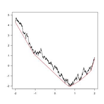
where C 𝐶 C V 𝑉 V ℝ ℝ \mathbb{R} V 𝑉 V [ − 2 , 2 ] 2 2 [-2,2] 1
Theorem 2.1
c − 1 / 2 { Q c − c E | C ( 0 ) | } ⟶ 𝒟 N ( 0 , σ 2 ) , c → ∞ , formulae-sequence superscript ⟶ 𝒟 superscript 𝑐 1 2 subscript 𝑄 𝑐 𝑐 𝐸 𝐶 0 𝑁 0 superscript 𝜎 2 → 𝑐 c^{-1/2}\left\{Q_{c}-cE|C(0)|\right\}\stackrel{{\scriptstyle{\cal D}}}{{\longrightarrow}}N(0,\sigma^{2}),\,c\to\infty,
where C ( 0 ) 𝐶 0 C(0) C 𝐶 C V 𝑉 V
σ 2 = 2 ∫ 0 ∞ covar ( − C ( 0 ) , V ( x ) − C ( x ) ) 𝑑 x . superscript 𝜎 2 2 superscript subscript 0 covar 𝐶 0 𝑉 𝑥 𝐶 𝑥 differential-d 𝑥 \sigma^{2}=2\int_{0}^{\infty}\mbox{\rm covar}(-C(0),V(x)-C(x))\,dx.
All moments of c − 1 / 2 { Q c − c E | C ( 0 ) | } superscript 𝑐 1 2 subscript 𝑄 𝑐 𝑐 𝐸 𝐶 0 c^{-1/2}\left\{Q_{c}-cE|C(0)|\right\} c 𝑐 c N ( 0 , σ 2 ) 𝑁 0 superscript 𝜎 2 N(0,\sigma^{2}) c → ∞ → 𝑐 c\to\infty
Figure 1: The greatest convex minorant of W ( x ) + x 2 𝑊 𝑥 superscript 𝑥 2 W(x)+x^{2} [ − 2 , 2 ] 2 2 [-2,2]
In the proof we will use the following lemma, which is proved in the appendix.
Lemma 2.1
For the process V 𝑉 V 2.4 c 𝑐 c c ′ superscript 𝑐 ′ c^{\prime} u ≥ 0 𝑢 0 u\geq 0
P ( min x ∉ [ − u , u ] V ( x ) ≤ 0 ) ≤ c e − c ′ u 3 . 𝑃 subscript 𝑥 𝑢 𝑢 𝑉 𝑥 0 𝑐 superscript 𝑒 superscript 𝑐 ′ superscript 𝑢 3 P\left(\min_{x\not\in[-u,u]}V(x)\leq 0\right)\leq ce^{-c^{\prime}u^{3}}.
Proof of Theorem 2.1
It follows from the results in [ Groeneboom (1989) ]
V ( x ) − C ( x ) , x ∈ ℝ , 𝑉 𝑥 𝐶 𝑥 𝑥
ℝ V(x)-C(x),\,x\in\mathbb{R}, (2.6)
is stationary. In fact, the process touches zero at changes of slope of C 𝐶 C
ϕ ( x ) = s − ( x − a ) 2 , x ∈ ℝ , formulae-sequence italic-ϕ 𝑥 𝑠 superscript 𝑥 𝑎 2 𝑥 ℝ \phi(x)=s-(x-a)^{2},\,x\in\mathbb{R},
where ϕ italic-ϕ \phi a 𝑎 a s 𝑠 s
D k = ∫ k k + 1 { V ( x ) − C ( x ) } 𝑑 x , k ∈ ℤ , formulae-sequence subscript 𝐷 𝑘 superscript subscript 𝑘 𝑘 1 𝑉 𝑥 𝐶 𝑥 differential-d 𝑥 𝑘 ℤ D_{k}=\int_{k}^{k+1}\left\{V(x)-C(x)\right\}\,dx,\,k\in{\mathbb{Z}},
we get a stationary sequence of random variables, and the stationarity of the process (2.6
E D k = ∫ k k + 1 E { V ( x ) − C ( x ) } 𝑑 x = E | C ( 0 ) | . 𝐸 subscript 𝐷 𝑘 superscript subscript 𝑘 𝑘 1 𝐸 𝑉 𝑥 𝐶 𝑥 differential-d 𝑥 𝐸 𝐶 0 ED_{k}=\int_{k}^{k+1}E\left\{V(x)-C(x)\right\}\,dx=E|C(0)|.
Moreover, all moments of D k subscript 𝐷 𝑘 D_{k}
max x ∈ [ 0 , 1 ] { V ( x ) − C ( x ) } subscript 𝑥 0 1 𝑉 𝑥 𝐶 𝑥 \max_{x\in[0,1]}\{V(x)-C(x)\}
has a distribution with tails which die out faster than exponentially. To see this, note that, ∀ u ≥ 0 for-all 𝑢 0 \forall u\geq 0
ℙ { max x ∈ [ 0 , 1 ] { V ( x ) − C ( x ) } ≥ M } ≤ ℙ { max x ∈ [ 0 , 1 ] V ( x ) ≥ 1 2 M } + ℙ { min x ∈ ℝ C ( x ) ≤ − 1 2 M } ℙ subscript 𝑥 0 1 𝑉 𝑥 𝐶 𝑥 𝑀 ℙ subscript 𝑥 0 1 𝑉 𝑥 1 2 𝑀 ℙ subscript 𝑥 ℝ 𝐶 𝑥 1 2 𝑀 \displaystyle{\mathbb{P}}\left\{\max_{x\in[0,1]}\{V(x)-C(x)\}\geq M\right\}\leq{\mathbb{P}}\left\{\max_{x\in[0,1]}V(x)\geq\tfrac{1}{2}M\right\}+{\mathbb{P}}\left\{\min_{x\in\mathbb{R}}C(x)\leq-\tfrac{1}{2}M\right\}
≤ ℙ { max x ∈ [ 0 , 1 ] W ( x ) ≥ 1 2 M − 1 } + ℙ { min x ∈ ℝ V ( x ) ≤ − 1 2 M } absent ℙ subscript 𝑥 0 1 𝑊 𝑥 1 2 𝑀 1 ℙ subscript 𝑥 ℝ 𝑉 𝑥 1 2 𝑀 \displaystyle\leq{\mathbb{P}}\left\{\max_{x\in[0,1]}W(x)\geq\tfrac{1}{2}M-1\right\}+{\mathbb{P}}\left\{\min_{x\in\mathbb{R}}V(x)\leq-\tfrac{1}{2}M\right\}
≤ 2 π ∫ 1 2 M − 1 ∞ e − 1 2 x 2 𝑑 x + ℙ { min x ∈ [ − u , u ] W ( x ) ≤ − 1 2 M } + ℙ { min x ∉ [ − u , u ] V ( x ) ≤ 0 } . absent 2 𝜋 superscript subscript 1 2 𝑀 1 superscript 𝑒 1 2 superscript 𝑥 2 differential-d 𝑥 ℙ subscript 𝑥 𝑢 𝑢 𝑊 𝑥 1 2 𝑀 ℙ subscript 𝑥 𝑢 𝑢 𝑉 𝑥 0 \displaystyle\leq\sqrt{\frac{2}{\pi}}\int_{\tfrac{1}{2}M-1}^{\infty}e^{-\tfrac{1}{2}x^{2}}\,dx+{\mathbb{P}}\left\{\min_{x\in[-u,u]}W(x)\leq-\tfrac{1}{2}M\right\}+{\mathbb{P}}\left\{\min_{x\notin[-u,u]}V(x)\leq 0\right\}. (2.7)
The first term on the right hand side is bounded by c exp { − c ′ M 2 / 4 } 𝑐 superscript 𝑐 ′ superscript 𝑀 2 4 c\exp\{-c^{\prime}M^{2}/4\} c , c ′ > 0 𝑐 superscript 𝑐 ′
0 c,c^{\prime}>0 2.1
P ( min x ∉ [ − u , u ] V ( x ) ≤ 0 ) ≤ c e − c ′ u 3 𝑃 subscript 𝑥 𝑢 𝑢 𝑉 𝑥 0 𝑐 superscript 𝑒 superscript 𝑐 ′ superscript 𝑢 3 P\left(\min_{x\not\in[-u,u]}V(x)\leq 0\right)\leq ce^{-c^{\prime}u^{3}}
for constants c , c ′ > 0 𝑐 superscript 𝑐 ′
0 c,c^{\prime}>0 2.7
ℙ { min x ∈ [ − u , u ] W ( x ) ≤ − M / 2 } = ℙ { min x ∈ [ − 1 , 1 ] W ( u x ) ≤ − M / 2 } ℙ subscript 𝑥 𝑢 𝑢 𝑊 𝑥 𝑀 2 ℙ subscript 𝑥 1 1 𝑊 𝑢 𝑥 𝑀 2 \displaystyle{\mathbb{P}}\left\{\min_{x\in[-u,u]}W(x)\leq-M/2\right\}={\mathbb{P}}\left\{\min_{x\in[-1,1]}W(ux)\leq-M/2\right\}
= ℙ { min x ∈ [ − 1 , 1 ] u − 1 / 2 W ( u x ) ≤ − u − 1 / 2 M / 2 } = ℙ { max x ∈ [ − 1 , 1 ] W ( x ) ≥ u − 1 / 2 M / 2 } absent ℙ subscript 𝑥 1 1 superscript 𝑢 1 2 𝑊 𝑢 𝑥 superscript 𝑢 1 2 𝑀 2 ℙ subscript 𝑥 1 1 𝑊 𝑥 superscript 𝑢 1 2 𝑀 2 \displaystyle={\mathbb{P}}\left\{\min_{x\in[-1,1]}u^{-1/2}W(ux)\leq-u^{-1/2}M/2\right\}={\mathbb{P}}\left\{\max_{x\in[-1,1]}W(x)\geq u^{-1/2}M/2\right\}
≤ 2 2 π ∫ u − 1 / 2 M / 2 ∞ e − 1 2 x 2 𝑑 x ≤ 2 2 π 2 u M exp { − 1 8 M 2 / u } . absent 2 2 𝜋 superscript subscript superscript 𝑢 1 2 𝑀 2 superscript 𝑒 1 2 superscript 𝑥 2 differential-d 𝑥 2 2 𝜋 2 𝑢 𝑀 1 8 superscript 𝑀 2 𝑢 \displaystyle\leq 2\sqrt{\frac{2}{\pi}}\int_{u^{-1/2}M/2}^{\infty}e^{-\tfrac{1}{2}x^{2}}\,dx\leq 2\sqrt{\frac{2}{\pi}}\frac{2\sqrt{u}}{M}\exp\left\{-\tfrac{1}{8}M^{2}/u\right\}.
Hence, taking u = M 𝑢 𝑀 u=\sqrt{M} 2.7
ℙ { max x ∈ [ 0 , 1 ] { V ( x ) − C ( x ) } ≥ M } ≤ c 1 e − c 2 M 3 / 2 ℙ subscript 𝑥 0 1 𝑉 𝑥 𝐶 𝑥 𝑀 subscript 𝑐 1 superscript 𝑒 subscript 𝑐 2 superscript 𝑀 3 2 {\mathbb{P}}\{\max_{x\in[0,1]}\{V(x)-C(x)\}\geq M\}\leq c_{1}e^{-c_{2}M^{3/2}} (2.8)
for constants c 1 , c 2 > 0 subscript 𝑐 1 subscript 𝑐 2
0 c_{1},c_{2}>0
Now let τ ( a ) 𝜏 𝑎 \tau(a)
τ ( a ) = argmin x ∈ ℝ { W ( x ) + ( x − a ) 2 } . 𝜏 𝑎 subscript argmin 𝑥 ℝ 𝑊 𝑥 superscript 𝑥 𝑎 2 \tau(a)=\mbox{argmin}_{x\in\mathbb{R}}\left\{W(x)+(x-a)^{2}\right\}.
The (stationary) process a ↦ τ ( a ) − a maps-to 𝑎 𝜏 𝑎 𝑎 a\mapsto\tau(a)-a [ Groeneboom (1989) ] c 1 subscript 𝑐 1 c_{1} c 2 subscript 𝑐 2 c_{2}
| ℙ ( A ∩ B ) − ℙ ( A ) ℙ ( B ) | ≤ c 1 e − c 2 m 3 , ℙ 𝐴 𝐵 ℙ 𝐴 ℙ 𝐵 subscript 𝑐 1 superscript 𝑒 subscript 𝑐 2 superscript 𝑚 3 |{\mathbb{P}}(A\cap B)-{\mathbb{P}}(A){\mathbb{P}}(B)|\leq c_{1}e^{-c_{2}m^{3}},
for events A 𝐴 A B 𝐵 B
A ∈ σ { τ ( a ) : a ≤ 0 } , B ∈ σ { τ ( a ) : a ≥ m } . formulae-sequence 𝐴 𝜎 conditional-set 𝜏 𝑎 𝑎 0 𝐵 𝜎 conditional-set 𝜏 𝑎 𝑎 𝑚 A\in\sigma\left\{\tau(a):a\leq 0\right\},\qquad B\in\sigma\left\{\tau(a):a\geq m\right\}.
This implies that there also exist positive constants c 1 subscript 𝑐 1 c_{1} c 2 subscript 𝑐 2 c_{2}
| ℙ ( A ∩ B ) − ℙ ( A ) ℙ ( B ) | ≤ c 1 e − c 2 m 3 , ℙ 𝐴 𝐵 ℙ 𝐴 ℙ 𝐵 subscript 𝑐 1 superscript 𝑒 subscript 𝑐 2 superscript 𝑚 3 |{\mathbb{P}}(A\cap B)-{\mathbb{P}}(A){\mathbb{P}}(B)|\leq c_{1}e^{-c_{2}m^{3}}, (2.9)
for events A 𝐴 A B 𝐵 B
A ∈ σ { V ( x ) − C ( x ) : x ≤ 0 } , B ∈ σ { V ( x ) − C ( x ) : x ≥ m } . formulae-sequence 𝐴 𝜎 conditional-set 𝑉 𝑥 𝐶 𝑥 𝑥 0 𝐵 𝜎 conditional-set 𝑉 𝑥 𝐶 𝑥 𝑥 𝑚 A\in\sigma\left\{V(x)-C(x):x\leq 0\right\},\qquad B\in\sigma\left\{V(x)-C(x):x\geq m\right\}.
So we can apply Theorem 18.5.3 in [ Ibragimow and Linnik (1971) ]
c − 1 / 2 { Q c − c E | C ( 0 ) | } ⟶ 𝒟 N ( 0 , σ 2 ) , superscript ⟶ 𝒟 superscript 𝑐 1 2 subscript 𝑄 𝑐 𝑐 𝐸 𝐶 0 𝑁 0 superscript 𝜎 2 c^{-1/2}\left\{Q_{c}-cE|C(0)|\right\}\stackrel{{\scriptstyle{\cal D}}}{{\longrightarrow}}N(0,\sigma^{2}),
where
σ 2 = var ( D 0 ) + 2 ∑ k = 1 ∞ covar ( D 0 , D k ) . superscript 𝜎 2 var subscript 𝐷 0 2 superscript subscript 𝑘 1 covar subscript 𝐷 0 subscript 𝐷 𝑘 \sigma^{2}={\rm var}(D_{0})+2\sum_{k=1}^{\infty}{\rm covar}(D_{0},D_{k}).
Using the stationarity of the process (2.6
σ 2 = 2 ∫ 0 ∞ covar ( − C ( 0 ) , V ( x ) − C ( x ) ) 𝑑 x . superscript 𝜎 2 2 superscript subscript 0 covar 𝐶 0 𝑉 𝑥 𝐶 𝑥 differential-d 𝑥 \sigma^{2}=2\int_{0}^{\infty}\mbox{\rm covar}(-C(0),V(x)-C(x))\,dx.
The last statement of the theorem follows from (2.8 2.9 □ □ \Box
We will also need the following extension of Theorem 2.1
Theorem 2.2
Let C c subscript 𝐶 𝑐 C_{c} [ 0 , c ] 0 𝑐 [0,c]
V ( x ) , x ∈ [ 0 , c ] . 𝑉 𝑥 𝑥
0 𝑐 V(x),\,x\in[0,c].
Note that C c subscript 𝐶 𝑐 C_{c} C 𝐶 C [ 0 , c ] 0 𝑐 [0,c] C 𝐶 C ℝ ℝ \mathbb{R} C c subscript 𝐶 𝑐 C_{c} V 𝑉 V [ 0 , c ] 0 𝑐 [0,c] [ 0 , c ] 0 𝑐 [0,c]
(i)
Let, for c > 4 𝑐 4 c>4 , the interval I c subscript 𝐼 𝑐 I_{c} be defined by
I c = [ c , c − c ] . subscript 𝐼 𝑐 𝑐 𝑐 𝑐 I_{c}=\left[\sqrt{c},c-\sqrt{c}\right].
Then:
c − 1 / 2 { ∫ I c { V ( x ) − C c ( x ) } 𝑑 x − E ∫ I c { V ( x ) − C c ( x ) } 𝑑 x } ⟶ 𝒟 N ( 0 , σ 2 ) , c → ∞ , formulae-sequence superscript ⟶ 𝒟 superscript 𝑐 1 2 subscript subscript 𝐼 𝑐 𝑉 𝑥 subscript 𝐶 𝑐 𝑥 differential-d 𝑥 𝐸 subscript subscript 𝐼 𝑐 𝑉 𝑥 subscript 𝐶 𝑐 𝑥 differential-d 𝑥 𝑁 0 superscript 𝜎 2 → 𝑐 c^{-1/2}\left\{\int_{I_{c}}\left\{V(x)-C_{c}(x)\right\}\,dx-E\int_{I_{c}}\left\{V(x)-C_{c}(x)\right\}\,dx\right\}\stackrel{{\scriptstyle{\cal D}}}{{\longrightarrow}}N(0,\sigma^{2}),\,c\to\infty, (2.10)
where σ 2 superscript 𝜎 2 \sigma^{2} is defined as in Theorem 2.1 .
(ii)
Relation ( 2.10 ) also holds if the interval I c subscript 𝐼 𝑐 I_{c} is given by:
I c = [ 0 , c − c ] or I c = [ c , c ] . subscript 𝐼 𝑐 0 𝑐 𝑐 or subscript 𝐼 𝑐 𝑐 𝑐 I_{c}=\left[0,c-\sqrt{c}\right]\mbox{ or }I_{c}=\left[\sqrt{c},c\right].
(iii)
For any choice of I c subscript 𝐼 𝑐 I_{c} in (i) or (ii), the fourth moment of
c − 1 / 2 { ∫ I c { V ( x ) − C c ( x ) } 𝑑 x − E ∫ I c { V ( x ) − C c ( x ) } 𝑑 x } superscript 𝑐 1 2 subscript subscript 𝐼 𝑐 𝑉 𝑥 subscript 𝐶 𝑐 𝑥 differential-d 𝑥 𝐸 subscript subscript 𝐼 𝑐 𝑉 𝑥 subscript 𝐶 𝑐 𝑥 differential-d 𝑥 c^{-1/2}\left\{\int_{I_{c}}\left\{V(x)-C_{c}(x)\right\}\,dx-E\int_{I_{c}}\left\{V(x)-C_{c}(x)\right\}\,dx\right\}
is uniformly bounded in c 𝑐 c , and converges to the fourth moment of a normal N ( 0 , σ 2 ) 𝑁 0 superscript 𝜎 2 N(0,\sigma^{2}) distribution, as c → ∞ → 𝑐 c\to\infty .
Proof. (i). The probability that C c subscript 𝐶 𝑐 C_{c} C 𝐶 C I c subscript 𝐼 𝑐 I_{c}
k 1 exp { − k 2 c 3 / 2 } , subscript 𝑘 1 subscript 𝑘 2 superscript 𝑐 3 2 k_{1}\exp\left\{-k_{2}c^{3/2}\right\},
for constants k 1 , k 2 > 0 subscript 𝑘 1 subscript 𝑘 2
0 k_{1},k_{2}>0 3.4 K c subscript 𝐾 𝑐 K_{c} C c ≢ C not-equivalent-to subscript 𝐶 𝑐 𝐶 C_{c}\not\equiv C I c subscript 𝐼 𝑐 I_{c}
E ∫ I c | C c ( x ) − C ( x ) | 𝑑 x ≤ { ∫ I c E { V ( x ) − C ( x ) } 2 𝑑 x } 1 / 2 ℙ ( K c ) 1 / 2 = O ( c 1 / 2 e − k c 3 / 2 ) , c → ∞ , formulae-sequence 𝐸 subscript subscript 𝐼 𝑐 subscript 𝐶 𝑐 𝑥 𝐶 𝑥 differential-d 𝑥 superscript subscript subscript 𝐼 𝑐 𝐸 superscript 𝑉 𝑥 𝐶 𝑥 2 differential-d 𝑥 1 2 ℙ superscript subscript 𝐾 𝑐 1 2 𝑂 superscript 𝑐 1 2 superscript 𝑒 𝑘 superscript 𝑐 3 2 → 𝑐 E\int_{I_{c}}\left|C_{c}(x)-C(x)\right|\,dx\leq\left\{\int_{I_{c}}E\left\{V(x)-C(x)\right\}^{2}\,dx\right\}^{1/2}{\mathbb{P}}(K_{c})^{1/2}=O\left(c^{1/2}e^{-kc^{3/2}}\right),\,c\to\infty,
for some k > 0 𝑘 0 k>0
c − 1 / 2 { ∫ I c { V ( x ) − C c ( x ) } 𝑑 x − E ∫ I c { V ( x ) − C c ( x ) } 𝑑 x } superscript 𝑐 1 2 subscript subscript 𝐼 𝑐 𝑉 𝑥 subscript 𝐶 𝑐 𝑥 differential-d 𝑥 𝐸 subscript subscript 𝐼 𝑐 𝑉 𝑥 subscript 𝐶 𝑐 𝑥 differential-d 𝑥 \displaystyle c^{-1/2}\left\{\int_{I_{c}}\left\{V(x)-C_{c}(x)\right\}\,dx-E\int_{I_{c}}\left\{V(x)-C_{c}(x)\right\}\,dx\right\}
= c − 1 / 2 { ∫ I c { V ( x ) − C ( x ) } 𝑑 x − E ∫ I c { V ( x ) − C ( x ) } 𝑑 x } + O p ( c e − k c 3 / 2 ) , absent superscript 𝑐 1 2 subscript subscript 𝐼 𝑐 𝑉 𝑥 𝐶 𝑥 differential-d 𝑥 𝐸 subscript subscript 𝐼 𝑐 𝑉 𝑥 𝐶 𝑥 differential-d 𝑥 subscript 𝑂 𝑝 𝑐 superscript 𝑒 𝑘 superscript 𝑐 3 2 \displaystyle=c^{-1/2}\left\{\int_{I_{c}}\left\{V(x)-C(x)\right\}\,dx-E\int_{I_{c}}\left\{V(x)-C(x)\right\}\,dx\right\}+O_{p}\left(ce^{-kc^{3/2}}\right),
and the statement now follows.
[ 0 , c ] 0 𝑐 [0,\sqrt{c}] I c ′ = [ c 1 / 4 , c − c 1 / 4 ] subscript superscript 𝐼 ′ 𝑐 superscript 𝑐 1 4 𝑐 superscript 𝑐 1 4 I^{\prime}_{c}=[c^{1/4},\sqrt{c}-c^{1/4}] C c subscript 𝐶 𝑐 C_{c}
c − 1 / 4 { ∫ I c ′ { V ( x ) − C c ( x ) } 𝑑 x − E ∫ I c ′ { V ( x ) − C c ( x ) } 𝑑 x } ⟶ 𝒟 N ( 0 , σ 2 ) , c → ∞ , formulae-sequence superscript ⟶ 𝒟 superscript 𝑐 1 4 subscript superscript subscript 𝐼 𝑐 ′ 𝑉 𝑥 subscript 𝐶 𝑐 𝑥 differential-d 𝑥 𝐸 subscript superscript subscript 𝐼 𝑐 ′ 𝑉 𝑥 subscript 𝐶 𝑐 𝑥 differential-d 𝑥 𝑁 0 superscript 𝜎 2 → 𝑐 c^{-1/4}\left\{\int_{I_{c}^{\prime}}\left\{V(x)-C_{c}(x)\right\}\,dx-E\int_{I_{c}^{\prime}}\left\{V(x)-C_{c}(x)\right\}\,dx\right\}\stackrel{{\scriptstyle{\cal D}}}{{\longrightarrow}}N(0,\sigma^{2}),\,c\to\infty,
implying:
c − 1 / 2 { ∫ I c ′ { V ( x ) − C c ( x ) } 𝑑 x − E ∫ I c ′ { V ( x ) − C c ( x ) } 𝑑 x } ⟶ p 0 , c → ∞ , formulae-sequence superscript ⟶ 𝑝 superscript 𝑐 1 2 subscript superscript subscript 𝐼 𝑐 ′ 𝑉 𝑥 subscript 𝐶 𝑐 𝑥 differential-d 𝑥 𝐸 subscript superscript subscript 𝐼 𝑐 ′ 𝑉 𝑥 subscript 𝐶 𝑐 𝑥 differential-d 𝑥 0 → 𝑐 c^{-1/2}\left\{\int_{I_{c}^{\prime}}\left\{V(x)-C_{c}(x)\right\}\,dx-E\int_{I_{c}^{\prime}}\left\{V(x)-C_{c}(x)\right\}\,dx\right\}\stackrel{{\scriptstyle p}}{{\longrightarrow}}0,\,c\to\infty,
Moreover,
c − 1 / 2 ∫ [ 0 , c 1 / 4 ] E | V ( x ) − C c ( x ) | 𝑑 x = O ( c − 1 / 4 ) , c → ∞ . formulae-sequence superscript 𝑐 1 2 subscript 0 superscript 𝑐 1 4 𝐸 𝑉 𝑥 subscript 𝐶 𝑐 𝑥 differential-d 𝑥 𝑂 superscript 𝑐 1 4 → 𝑐 c^{-1/2}\int_{[0,c^{1/4}]}E\left|V(x)-C_{c}(x)\right|\,dx=O\left(c^{-1/4}\right),\,c\to\infty.
The statement now follows for the first choice of the interval I c subscript 𝐼 𝑐 I_{c} I c subscript 𝐼 𝑐 I_{c} I c subscript 𝐼 𝑐 I_{c}
c − 2 E { ∫ I c { V ( x ) − C c ( x ) } 𝑑 x − E ∫ I c { V ( x ) − C c ( x ) } 𝑑 x } 4 superscript 𝑐 2 𝐸 superscript subscript subscript 𝐼 𝑐 𝑉 𝑥 subscript 𝐶 𝑐 𝑥 differential-d 𝑥 𝐸 subscript subscript 𝐼 𝑐 𝑉 𝑥 subscript 𝐶 𝑐 𝑥 differential-d 𝑥 4 \displaystyle c^{-2}E\left\{\int_{I_{c}}\left\{V(x)-C_{c}(x)\right\}\,dx-E\int_{I_{c}}\left\{V(x)-C_{c}(x)\right\}\,dx\right\}^{4}
= c − 2 E { ∫ I c { V ( x ) − C ( x ) } 𝑑 x − E ∫ I c { V ( x ) − C ( x ) } 𝑑 x } 4 + O ( e − k c 3 / 2 ) , absent superscript 𝑐 2 𝐸 superscript subscript subscript 𝐼 𝑐 𝑉 𝑥 𝐶 𝑥 differential-d 𝑥 𝐸 subscript subscript 𝐼 𝑐 𝑉 𝑥 𝐶 𝑥 differential-d 𝑥 4 𝑂 superscript 𝑒 𝑘 superscript 𝑐 3 2 \displaystyle=c^{-2}E\left\{\int_{I_{c}}\left\{V(x)-C(x)\right\}\,dx-E\int_{I_{c}}\left\{V(x)-C(x)\right\}\,dx\right\}^{4}+O\left(e^{-kc^{3/2}}\right),
for some k > 0 𝑘 0 k>0 2.1 2.8 2.9
( c c − 2 c ) 2 → 1 , c → ∞ . formulae-sequence → superscript 𝑐 𝑐 2 𝑐 2 1 → 𝑐 \left(\frac{c}{c-2\sqrt{c}}\right)^{2}\to 1,\,c\to\infty.
If, for example, I c = [ 0 , c − c ] subscript 𝐼 𝑐 0 𝑐 𝑐 I_{c}=[0,c-\sqrt{c}]
∫ I c { V ( x ) − C c ( x ) } 𝑑 x − E ∫ I c { V ( x ) − C c ( x ) } 𝑑 x = A c + B c , subscript subscript 𝐼 𝑐 𝑉 𝑥 subscript 𝐶 𝑐 𝑥 differential-d 𝑥 𝐸 subscript subscript 𝐼 𝑐 𝑉 𝑥 subscript 𝐶 𝑐 𝑥 differential-d 𝑥 subscript 𝐴 𝑐 subscript 𝐵 𝑐 \displaystyle\int_{I_{c}}\left\{V(x)-C_{c}(x)\right\}\,dx-E\int_{I_{c}}\left\{V(x)-C_{c}(x)\right\}\,dx=A_{c}+B_{c},
where
A c = ∫ [ 0 , c ] { V ( x ) − C c ( x ) } 𝑑 x − E ∫ [ 0 , c ] { V ( x ) − C c ( x ) } 𝑑 x subscript 𝐴 𝑐 subscript 0 𝑐 𝑉 𝑥 subscript 𝐶 𝑐 𝑥 differential-d 𝑥 𝐸 subscript 0 𝑐 𝑉 𝑥 subscript 𝐶 𝑐 𝑥 differential-d 𝑥 A_{c}=\int_{[0,\sqrt{c}]}\left\{V(x)-C_{c}(x)\right\}\,dx-E\int_{[0,\sqrt{c}]}\left\{V(x)-C_{c}(x)\right\}\,dx
and
B c = ∫ [ c , c − c ] { V ( x ) − C c ( x ) } 𝑑 x − E ∫ [ c , c − c ] { V ( x ) − C c ( x ) } 𝑑 x . subscript 𝐵 𝑐 subscript 𝑐 𝑐 𝑐 𝑉 𝑥 subscript 𝐶 𝑐 𝑥 differential-d 𝑥 𝐸 subscript 𝑐 𝑐 𝑐 𝑉 𝑥 subscript 𝐶 𝑐 𝑥 differential-d 𝑥 B_{c}=\int_{[\sqrt{c},c-\sqrt{c}]}\left\{V(x)-C_{c}(x)\right\}\,dx-E\int_{[\sqrt{c},c-\sqrt{c}]}\left\{V(x)-C_{c}(x)\right\}\,dx.
Hence we get:
c − 2 E { ∫ I c { V ( x ) − C c ( x ) } 𝑑 x − E ∫ I c { V ( x ) − C c ( x ) } 𝑑 x } 4 superscript 𝑐 2 𝐸 superscript subscript subscript 𝐼 𝑐 𝑉 𝑥 subscript 𝐶 𝑐 𝑥 differential-d 𝑥 𝐸 subscript subscript 𝐼 𝑐 𝑉 𝑥 subscript 𝐶 𝑐 𝑥 differential-d 𝑥 4 \displaystyle c^{-2}E\left\{\int_{I_{c}}\left\{V(x)-C_{c}(x)\right\}\,dx-E\int_{I_{c}}\left\{V(x)-C_{c}(x)\right\}\,dx\right\}^{4}
= c − 2 E B c 4 + c − 2 { 4 E B c 3 A c + 6 E B c 2 A c 2 + 4 E B c A c 3 + E A c 4 } . absent superscript 𝑐 2 𝐸 superscript subscript 𝐵 𝑐 4 superscript 𝑐 2 4 𝐸 superscript subscript 𝐵 𝑐 3 subscript 𝐴 𝑐 6 𝐸 superscript subscript 𝐵 𝑐 2 superscript subscript 𝐴 𝑐 2 4 𝐸 subscript 𝐵 𝑐 superscript subscript 𝐴 𝑐 3 𝐸 superscript subscript 𝐴 𝑐 4 \displaystyle=c^{-2}EB_{c}^{4}+c^{-2}\left\{4EB_{c}^{3}A_{c}+6EB_{c}^{2}A_{c}^{2}+4EB_{c}A_{c}^{3}+EA_{c}^{4}\right\}.
We have:
c − 2 E A c 4 = ( c c ) 2 c − 1 E A c 4 = O ( c − 1 ) , superscript 𝑐 2 𝐸 superscript subscript 𝐴 𝑐 4 superscript 𝑐 𝑐 2 superscript 𝑐 1 𝐸 superscript subscript 𝐴 𝑐 4 𝑂 superscript 𝑐 1 c^{-2}EA_{c}^{4}=\left(\frac{\sqrt{c}}{c}\right)^{2}c^{-1}EA_{c}^{4}=O\left(c^{-1}\right),
and similarly, using the Cauchy-Schwarz inequality,
c − 2 E B c A c 3 = E c − 3 / 2 A c 3 c − 1 / 2 B c ≤ E c − 3 A c 6 E c − 1 B c 2 = O ( c − 3 / 4 ) . superscript 𝑐 2 𝐸 subscript 𝐵 𝑐 superscript subscript 𝐴 𝑐 3 𝐸 superscript 𝑐 3 2 superscript subscript 𝐴 𝑐 3 superscript 𝑐 1 2 subscript 𝐵 𝑐 𝐸 superscript 𝑐 3 superscript subscript 𝐴 𝑐 6 𝐸 superscript 𝑐 1 superscript subscript 𝐵 𝑐 2 𝑂 superscript 𝑐 3 4 c^{-2}EB_{c}A_{c}^{3}=Ec^{-3/2}A_{c}^{3}c^{-1/2}B_{c}\leq\sqrt{Ec^{-3}A_{c}^{6}}\sqrt{Ec^{-1}B_{c}^{2}}=O\left(c^{-3/4}\right).
Continuing in this way, we find that the only non-vanishing term is c − 2 E B c 4 superscript 𝑐 2 𝐸 superscript subscript 𝐵 𝑐 4 c^{-2}EB_{c}^{4} I c = [ c , c − c ] subscript 𝐼 𝑐 𝑐 𝑐 𝑐 I_{c}=[\sqrt{c},c-\sqrt{c}] □ □ \Box
We finally also need the following extension of Theorem 2.2
Theorem 2.3
Let F c subscript 𝐹 𝑐 F_{c} G c subscript 𝐺 𝑐 G_{c} H c subscript 𝐻 𝑐 H_{c} [ 0 , c ] 0 𝑐 [0,c] f c subscript 𝑓 𝑐 f_{c} g c subscript 𝑔 𝑐 g_{c} h c subscript ℎ 𝑐 h_{c}
F c ( x ) = f c ( 0 ) x ( 1 + o ( 1 ) ) , G c ( x ) = g c ( 0 ) x ( 1 + o ( 1 ) ) , H c ( x ) = 1 2 h c ′ ( 0 ) x 2 ( 1 + o ( 1 ) ) , c → ∞ , formulae-sequence subscript 𝐹 𝑐 𝑥 subscript 𝑓 𝑐 0 𝑥 1 𝑜 1 formulae-sequence subscript 𝐺 𝑐 𝑥 subscript 𝑔 𝑐 0 𝑥 1 𝑜 1 formulae-sequence subscript 𝐻 𝑐 𝑥 1 2 superscript subscript ℎ 𝑐 ′ 0 superscript 𝑥 2 1 𝑜 1 → 𝑐 F_{c}(x)=f_{c}(0)x(1+o(1)),\qquad G_{c}(x)=g_{c}(0)x(1+o(1)),\qquad H_{c}(x)=\tfrac{1}{2}h_{c}^{\prime}(0)x^{2}(1+o(1)),\,c\to\infty,
where the o ( 1 ) 𝑜 1 o(1) x 𝑥 x f c ( 0 ) subscript 𝑓 𝑐 0 f_{c}(0) g c ( 0 ) subscript 𝑔 𝑐 0 g_{c}(0) h c ( 0 ) subscript ℎ 𝑐 0 h_{c}(0) h c ′ ( 0 ) superscript subscript ℎ 𝑐 ′ 0 h_{c}^{\prime}(0) ∞ \infty c → ∞ → 𝑐 c\to\infty h c ′ ( 0 ) superscript subscript ℎ 𝑐 ′ 0 h_{c}^{\prime}(0) h c subscript ℎ 𝑐 h_{c} C c subscript 𝐶 𝑐 C_{c} [ 0 , c ] 0 𝑐 [0,c]
V c ( x ) = H c ( x ) + W ( G c ( x ) ) , x ∈ [ 0 , c ] . formulae-sequence subscript 𝑉 𝑐 𝑥 subscript 𝐻 𝑐 𝑥 𝑊 subscript 𝐺 𝑐 𝑥 𝑥 0 𝑐 V_{c}(x)=H_{c}(x)+W(G_{c}(x)),\,x\in[0,c].
Moreover, let S c subscript 𝑆 𝑐 S_{c}
S c ( x ) = V c ( x ) − C c ( x ) , x ∈ [ 0 , c ] . formulae-sequence subscript 𝑆 𝑐 𝑥 subscript 𝑉 𝑐 𝑥 subscript 𝐶 𝑐 𝑥 𝑥 0 𝑐 S_{c}(x)=V_{c}(x)-C_{c}(x),\,x\in[0,c].
Then:
(i)
Let, for c > 4 𝑐 4 c>4 , the interval I c subscript 𝐼 𝑐 I_{c} be defined by
I c = [ c , c − c ] . subscript 𝐼 𝑐 𝑐 𝑐 𝑐 I_{c}=\left[\sqrt{c},c-\sqrt{c}\right].
Then:
c − 1 E ∫ I c S c ( x ) 𝑑 F c ( x ) ∼ g c ( 0 ) 2 / 3 f c ( 0 ) ( 1 2 h c ′ ( 0 ) ) 1 / 3 E | C ( 0 ) | , var ( c − 1 / 2 ∫ I c S c ( x ) 𝑑 F c ( x ) ) ∼ σ c 2 , c → ∞ , formulae-sequence similar-to superscript 𝑐 1 𝐸 subscript subscript 𝐼 𝑐 subscript 𝑆 𝑐 𝑥 differential-d subscript 𝐹 𝑐 𝑥 subscript 𝑔 𝑐 superscript 0 2 3 subscript 𝑓 𝑐 0 superscript 1 2 superscript subscript ℎ 𝑐 ′ 0 1 3 𝐸 𝐶 0 formulae-sequence similar-to var superscript 𝑐 1 2 subscript subscript 𝐼 𝑐 subscript 𝑆 𝑐 𝑥 differential-d subscript 𝐹 𝑐 𝑥 superscript subscript 𝜎 𝑐 2 → 𝑐 c^{-1}E\int_{I_{c}}S_{c}(x)\,dF_{c}(x)\sim\frac{g_{c}(0)^{2/3}f_{c}(0)}{\left(\tfrac{1}{2}h_{c}^{\prime}(0)\right)^{1/3}}E|C(0)|,\,\mbox{\rm var}\left(c^{-1/2}\int_{I_{c}}S_{c}(x)\,dF_{c}(x)\right)\sim\sigma_{c}^{2},\,c\to\infty, (2.11)
where
σ c 2 = g c ( 0 ) 5 / 3 f c ( 0 ) 2 ( 1 2 h c ′ ( 0 ) ) 4 / 3 σ 2 , superscript subscript 𝜎 𝑐 2 subscript 𝑔 𝑐 superscript 0 5 3 subscript 𝑓 𝑐 superscript 0 2 superscript 1 2 superscript subscript ℎ 𝑐 ′ 0 4 3 superscript 𝜎 2 \sigma_{c}^{2}=\frac{g_{c}(0)^{5/3}f_{c}(0)^{2}}{\left(\tfrac{1}{2}h_{c}^{\prime}(0)\right)^{4/3}}\sigma^{2}, (2.12)
and C 𝐶 C and σ 2 superscript 𝜎 2 \sigma^{2} are defined as in Theorem 2.1 . Moreover, the fourth moment of
c − 1 / 2 ∫ I c { S c ( x ) − E S c ( x ) } 𝑑 F c ( x ) superscript 𝑐 1 2 subscript subscript 𝐼 𝑐 subscript 𝑆 𝑐 𝑥 𝐸 subscript 𝑆 𝑐 𝑥 differential-d subscript 𝐹 𝑐 𝑥 c^{-1/2}\int_{I_{c}}\left\{S_{c}(x)-ES_{c}(x)\right\}\,dF_{c}(x)
is uniformly bounded, and satisfies:
E ( c − 1 / 2 ∫ I c { S c ( x ) − E S c ( x ) } 𝑑 F c ( x ) ) 4 ∼ M c ( 4 ) , c → ∞ , formulae-sequence similar-to 𝐸 superscript superscript 𝑐 1 2 subscript subscript 𝐼 𝑐 subscript 𝑆 𝑐 𝑥 𝐸 subscript 𝑆 𝑐 𝑥 differential-d subscript 𝐹 𝑐 𝑥 4 superscript subscript 𝑀 𝑐 4 → 𝑐 E\left(c^{-1/2}\int_{I_{c}}\left\{S_{c}(x)-ES_{c}(x)\right\}\,dF_{c}(x)\right)^{4}\sim M_{c}^{(4)},\,c\to\infty, (2.13)
where M c ( 4 ) superscript subscript 𝑀 𝑐 4 M_{c}^{(4)} denotes the fourth moment of a normal N ( 0 , σ c 2 ) 𝑁 0 superscript subscript 𝜎 𝑐 2 N(0,\sigma_{c}^{2}) distribution.
(ii)
Relations ( 2.11 ) and ( 2.13 ) also hold if the interval I c subscript 𝐼 𝑐 I_{c} is given by:
I c = [ 0 , c − c ] , I c = [ c , c ] or I c = [ 0 , c ] . formulae-sequence subscript 𝐼 𝑐 0 𝑐 𝑐 subscript 𝐼 𝑐 𝑐 𝑐 or subscript 𝐼 𝑐 0 𝑐 I_{c}=\left[0,c-\sqrt{c}\right],\,I_{c}=\left[\sqrt{c},c\right]\mbox{ or }I_{c}=[0,c].
Proof. Since the proof proceeds along the lines of the proofs of Theorems 2.1 2.2
x ↦ 1 2 h c ′ ( 0 ) x 2 + W ( g c ( 0 ) x ) , x ∈ [ 0 , c ] , formulae-sequence maps-to 𝑥 1 2 superscript subscript ℎ 𝑐 ′ 0 superscript 𝑥 2 𝑊 subscript 𝑔 𝑐 0 𝑥 𝑥 0 𝑐 x\mapsto\tfrac{1}{2}h_{c}^{\prime}(0)x^{2}+W(g_{c}(0)x),\,x\in[0,c],
which replaces the process
x ↦ V ( x ) = x 2 + W ( x ) , x ∈ [ 0 , c ] . formulae-sequence maps-to 𝑥 𝑉 𝑥 superscript 𝑥 2 𝑊 𝑥 𝑥 0 𝑐 x\mapsto V(x)=x^{2}+W(x),\,x\in[0,c].
Let a , b > 0 𝑎 𝑏
0 a,b>0
x ↦ a x 2 + W ( b x ) , x ∈ [ 0 , c ] , formulae-sequence maps-to 𝑥 𝑎 superscript 𝑥 2 𝑊 𝑏 𝑥 𝑥 0 𝑐 x\mapsto ax^{2}+W(bx),\,x\in[0,c], (2.14)
has the same distribution as the process
x ↦ a − 1 / 3 b 2 / 3 { ( a 2 / 3 b − 1 / 3 x ) 2 + W ( a 2 / 3 b − 1 / 3 x ) } , x ∈ [ 0 , c ] . formulae-sequence maps-to 𝑥 superscript 𝑎 1 3 superscript 𝑏 2 3 superscript superscript 𝑎 2 3 superscript 𝑏 1 3 𝑥 2 𝑊 superscript 𝑎 2 3 superscript 𝑏 1 3 𝑥 𝑥 0 𝑐 x\mapsto a^{-1/3}b^{2/3}\left\{\left(a^{2/3}b^{-1/3}x\right)^{2}+W(a^{2/3}b^{-1/3}x)\right\},\,x\in[0,c]. (2.15)
Hence, if C a , b subscript 𝐶 𝑎 𝑏
C_{a,b} 2.14 C ~ a , b subscript ~ 𝐶 𝑎 𝑏
\tilde{C}_{a,b} 2.15
∫ 0 c { a x 2 + W ( b x ) − C a , b ( x ) } f c ( 0 ) 𝑑 x superscript subscript 0 𝑐 𝑎 superscript 𝑥 2 𝑊 𝑏 𝑥 subscript 𝐶 𝑎 𝑏
𝑥 subscript 𝑓 𝑐 0 differential-d 𝑥 \displaystyle\int_{0}^{c}\left\{ax^{2}+W(bx)-C_{a,b}(x)\right\}f_{c}(0)\,dx
= 𝒟 a − 1 / 3 b 2 / 3 f c ( 0 ) ∫ 0 c { ( a 2 / 3 b − 1 / 3 x ) 2 + W ( a 2 / 3 b − 1 / 3 x ) − a 1 / 3 b − 2 / 3 C ~ a , b ( x ) } 𝑑 x superscript 𝒟 superscript 𝑎 1 3 superscript 𝑏 2 3 subscript 𝑓 𝑐 0 superscript subscript 0 𝑐 superscript superscript 𝑎 2 3 superscript 𝑏 1 3 𝑥 2 𝑊 superscript 𝑎 2 3 superscript 𝑏 1 3 𝑥 superscript 𝑎 1 3 superscript 𝑏 2 3 subscript ~ 𝐶 𝑎 𝑏
𝑥 differential-d 𝑥 \displaystyle\mathop{\rm=}^{\cal D}a^{-1/3}b^{2/3}f_{c}(0)\int_{0}^{c}\left\{\left(a^{2/3}b^{-1/3}x\right)^{2}+W(a^{2/3}b^{-1/3}x)-a^{1/3}b^{-2/3}\tilde{C}_{a,b}(x)\right\}\,dx
= b f c ( 0 ) a ∫ 0 a 2 / 3 b − 1 / 3 c { u 2 + W ( u ) − a 1 / 3 b − 2 / 3 C ~ a , b ( a − 2 / 3 b 1 / 3 u ) } 𝑑 u absent 𝑏 subscript 𝑓 𝑐 0 𝑎 superscript subscript 0 superscript 𝑎 2 3 superscript 𝑏 1 3 𝑐 superscript 𝑢 2 𝑊 𝑢 superscript 𝑎 1 3 superscript 𝑏 2 3 subscript ~ 𝐶 𝑎 𝑏
superscript 𝑎 2 3 superscript 𝑏 1 3 𝑢 differential-d 𝑢 \displaystyle=\frac{bf_{c}(0)}{a}\int_{0}^{a^{2/3}b^{-1/3}c}\left\{u^{2}+W(u)-a^{1/3}b^{-2/3}\tilde{C}_{a,b}\left(a^{-2/3}b^{1/3}u\right)\right\}\,du
= b f c ( 0 ) a ∫ 0 a 2 / 3 b − 1 / 3 c { u 2 + W ( u ) − C c ( u ) } 𝑑 u , absent 𝑏 subscript 𝑓 𝑐 0 𝑎 superscript subscript 0 superscript 𝑎 2 3 superscript 𝑏 1 3 𝑐 superscript 𝑢 2 𝑊 𝑢 subscript 𝐶 𝑐 𝑢 differential-d 𝑢 \displaystyle=\frac{bf_{c}(0)}{a}\int_{0}^{a^{2/3}b^{-1/3}c}\left\{u^{2}+W(u)-C_{c}(u)\right\}\,du,
where C c subscript 𝐶 𝑐 C_{c}
u ↦ u 2 + W ( u ) , u ∈ [ 0 , a 2 / 3 b − 1 / 3 c ] . formulae-sequence maps-to 𝑢 superscript 𝑢 2 𝑊 𝑢 𝑢 0 superscript 𝑎 2 3 superscript 𝑏 1 3 𝑐 u\mapsto u^{2}+W(u),\,u\in\left[0,a^{2/3}b^{-1/3}c\right].
Thus, for c → ∞ → 𝑐 c\rightarrow\infty
c − 1 E ∫ 0 c { a x 2 + W ( b x ) − C a , b ( x ) } f c ( 0 ) 𝑑 x ∼ b 2 / 3 f c ( 0 ) a 1 / 3 E | C ( 0 ) | . similar-to superscript 𝑐 1 𝐸 superscript subscript 0 𝑐 𝑎 superscript 𝑥 2 𝑊 𝑏 𝑥 subscript 𝐶 𝑎 𝑏
𝑥 subscript 𝑓 𝑐 0 differential-d 𝑥 superscript 𝑏 2 3 subscript 𝑓 𝑐 0 superscript 𝑎 1 3 𝐸 𝐶 0 \displaystyle c^{-1}E\int_{0}^{c}\left\{ax^{2}+W(bx)-C_{a,b}(x)\right\}f_{c}(0)\,dx\sim\frac{b^{2/3}f_{c}(0)}{a^{1/3}}E|C(0)|.
Using that a = 1 2 h c ′ ( 0 ) 𝑎 1 2 superscript subscript ℎ 𝑐 ′ 0 a=\tfrac{1}{2}h_{c}^{\prime}(0) b = g c ( 0 ) 𝑏 subscript 𝑔 𝑐 0 b=g_{c}(0) 2.11
var ( c − 1 / 2 ∫ 0 c { a x 2 + W ( b x ) − C a , b ( x ) } f c ( 0 ) 𝑑 u ) var superscript 𝑐 1 2 superscript subscript 0 𝑐 𝑎 superscript 𝑥 2 𝑊 𝑏 𝑥 subscript 𝐶 𝑎 𝑏
𝑥 subscript 𝑓 𝑐 0 differential-d 𝑢 \displaystyle\mbox{var}\left(c^{-1/2}\int_{0}^{c}\left\{ax^{2}+W(bx)-C_{a,b}(x)\right\}f_{c}(0)\,du\right)
= b 2 f c ( 0 ) 2 a 2 c var ( ∫ 0 a 2 / 3 b − 1 / 3 c { u 2 + W ( u ) − C c ( u ) } 𝑑 u ) absent superscript 𝑏 2 subscript 𝑓 𝑐 superscript 0 2 superscript 𝑎 2 𝑐 var superscript subscript 0 superscript 𝑎 2 3 superscript 𝑏 1 3 𝑐 superscript 𝑢 2 𝑊 𝑢 subscript 𝐶 𝑐 𝑢 differential-d 𝑢 \displaystyle=\frac{b^{2}f_{c}(0)^{2}}{a^{2}c}\mbox{var}\left(\int_{0}^{a^{2/3}b^{-1/3}c}\left\{u^{2}+W(u)-C_{c}(u)\right\}\,du\right)
= b 5 / 3 f c ( 0 ) 2 a 4 / 3 var ( 1 b − 1 / 3 a 2 / 3 c ∫ 0 a 2 / 3 b − 1 / 3 c { u 2 + W ( u ) − C c ( u ) } 𝑑 u ) absent superscript 𝑏 5 3 subscript 𝑓 𝑐 superscript 0 2 superscript 𝑎 4 3 var 1 superscript 𝑏 1 3 superscript 𝑎 2 3 𝑐 superscript subscript 0 superscript 𝑎 2 3 superscript 𝑏 1 3 𝑐 superscript 𝑢 2 𝑊 𝑢 subscript 𝐶 𝑐 𝑢 differential-d 𝑢 \displaystyle=\frac{b^{5/3}f_{c}(0)^{2}}{a^{4/3}}\mbox{var}\left(\frac{1}{\sqrt{b^{-1/3}a^{2/3}c}}\int_{0}^{a^{2/3}b^{-1/3}c}\left\{u^{2}+W(u)-C_{c}(u)\right\}\,du\right)
∼ b 5 / 3 f c ( 0 ) 2 a 4 / 3 σ 2 c → ∞ . similar-to absent superscript 𝑏 5 3 subscript 𝑓 𝑐 superscript 0 2 superscript 𝑎 4 3 superscript 𝜎 2 𝑐 → \displaystyle\sim\frac{b^{5/3}f_{c}(0)^{2}}{a^{4/3}}\sigma^{2}\,c\to\infty.
Taking a = 1 2 h c ′ ( 0 ) 𝑎 1 2 superscript subscript ℎ 𝑐 ′ 0 a=\tfrac{1}{2}h_{c}^{\prime}(0) b = g c ( 0 ) 𝑏 subscript 𝑔 𝑐 0 b=g_{c}(0) 2.12 □ □ \Box
3 Embedding and first central limit result
In this section, a central limit result is established for the quantity
n 5 / 6 ∫ 0 a { ℍ n ( x ) − H ^ n ( x ) − μ n } 𝑑 F 0 ( x ) = n 5 / 6 ∫ 0 a { ℍ n ( x − ) − H ^ n ( x ) − μ n } 𝑑 F 0 ( x ) , superscript 𝑛 5 6 superscript subscript 0 𝑎 subscript ℍ 𝑛 𝑥 subscript ^ 𝐻 𝑛 𝑥 subscript 𝜇 𝑛 differential-d subscript 𝐹 0 𝑥 superscript 𝑛 5 6 superscript subscript 0 𝑎 subscript ℍ 𝑛 limit-from 𝑥 subscript ^ 𝐻 𝑛 𝑥 subscript 𝜇 𝑛 differential-d subscript 𝐹 0 𝑥 n^{5/6}\int_{0}^{a}\left\{{\mathbb{H}}_{n}(x)-\hat{H}_{n}(x)-\mu_{n}\right\}\,dF_{0}(x)=n^{5/6}\int_{0}^{a}\left\{{\mathbb{H}}_{n}(x-)-\hat{H}_{n}(x)-\mu_{n}\right\}\,dF_{0}(x), (3.16)
where μ n subscript 𝜇 𝑛 \mu_{n} T n subscript 𝑇 𝑛 T_{n} 1.1 d 𝔽 n 𝑑 subscript 𝔽 𝑛 d{\mathbb{F}}_{n} d F 0 𝑑 subscript 𝐹 0 dF_{0} 3.16 ℍ n ( x ) − H ^ n ( x ) subscript ℍ 𝑛 𝑥 subscript ^ 𝐻 𝑛 𝑥 {\mathbb{H}}_{n}(x)-\hat{H}_{n}(x)
x ↦ H 0 ( x ) + E n ( x ) n { 1 − F 0 ( x ) − H ~ n ( x ) , x ∈ [ 0 , a ] . x\mapsto H_{0}(x)+\frac{E_{n}(x)}{\sqrt{n}\{1-F_{0}(x)}-\tilde{H}_{n}(x),\,x\in[0,a].
where E n subscript 𝐸 𝑛 E_{n} n { 𝔽 n − F 0 } 𝑛 subscript 𝔽 𝑛 subscript 𝐹 0 \sqrt{n}\{{\mathbb{F}}_{n}-F_{0}\} H ~ n subscript ~ 𝐻 𝑛 \tilde{H}_{n}
x ↦ H 0 ( x ) + n − 1 / 2 E n ( x ) / { 1 − F 0 ( x ) } , x ∈ [ 0 , a ] . formulae-sequence maps-to 𝑥 subscript 𝐻 0 𝑥 superscript 𝑛 1 2 subscript 𝐸 𝑛 𝑥 1 subscript 𝐹 0 𝑥 𝑥 0 𝑎 x\mapsto H_{0}(x)+n^{-1/2}E_{n}(x)/\{1-F_{0}(x)\}\,,\,x\in[0,a]. (3.17)
Next we use the strong approximation of the empirical process by a Brownian bridge B n subscript 𝐵 𝑛 B_{n}
x ↦ H 0 ( x ) + n − 1 / 2 B n ( F 0 ( x ) ) 1 − F 0 ( x ) , x ∈ [ 0 , a ] , formulae-sequence maps-to 𝑥 subscript 𝐻 0 𝑥 superscript 𝑛 1 2 subscript 𝐵 𝑛 subscript 𝐹 0 𝑥 1 subscript 𝐹 0 𝑥 𝑥 0 𝑎 x\mapsto H_{0}(x)+\frac{n^{-1/2}B_{n}(F_{0}(x))}{1-F_{0}(x)},\,x\in[0,a],
the process (3.17
x ↦ H 0 ( x ) + n − 1 / 2 W ( F 0 ( x ) 1 − F 0 ( x ) ) , x ∈ [ 0 , a ] , formulae-sequence maps-to 𝑥 subscript 𝐻 0 𝑥 superscript 𝑛 1 2 𝑊 subscript 𝐹 0 𝑥 1 subscript 𝐹 0 𝑥 𝑥 0 𝑎 x\mapsto H_{0}(x)+n^{-1/2}W\left(\frac{F_{0}(x)}{1-F_{0}(x)}\right),\,x\in[0,a], (3.18)
where W 𝑊 W [ 0 , ∞ ) 0 [0,\infty) [ 0 , a ] 0 𝑎 [0,a] 2
The first lemma to be proved states a contraction property for convex minorants that will be used repeatedly in the sequel. It is related to Marshall’s Lemma in the theory of isotonic regression.
Lemma 3.1
Let f 𝑓 f g 𝑔 g I ⊂ ℝ 𝐼 ℝ I\subset\mathbb{R} C f subscript 𝐶 𝑓 C_{f} C g subscript 𝐶 𝑔 C_{g}
sup x ∈ I | C f ( x ) − C g ( x ) | ≤ sup x ∈ I | f ( x ) − g ( x ) | . subscript supremum 𝑥 𝐼 subscript 𝐶 𝑓 𝑥 subscript 𝐶 𝑔 𝑥 subscript supremum 𝑥 𝐼 𝑓 𝑥 𝑔 𝑥 \sup_{x\in I}\left|C_{f}(x)-C_{g}(x)\right|\leq\sup_{x\in I}|f(x)-g(x)|.
Proof. Using that f ≥ g − sup u ∈ I | f ( u ) − g ( u ) | 𝑓 𝑔 subscript supremum 𝑢 𝐼 𝑓 𝑢 𝑔 𝑢 f\geq g-\sup_{u\in I}|f(u)-g(u)| g ≥ C g 𝑔 subscript 𝐶 𝑔 g\geq C_{g} f ≥ C g − sup u ∈ I | f ( u ) − g ( u ) | 𝑓 subscript 𝐶 𝑔 subscript supremum 𝑢 𝐼 𝑓 𝑢 𝑔 𝑢 f\geq C_{g}-\sup_{u\in I}|f(u)-g(u)| a convex minorant of f 𝑓 f I 𝐼 I C f subscript 𝐶 𝑓 C_{f} f 𝑓 f I 𝐼 I
C f ( x ) ≥ C g ( x ) − sup u ∈ I | f ( u ) − g ( u ) | , x ∈ I . formulae-sequence subscript 𝐶 𝑓 𝑥 subscript 𝐶 𝑔 𝑥 subscript supremum 𝑢 𝐼 𝑓 𝑢 𝑔 𝑢 𝑥 𝐼 C_{f}(x)\geq C_{g}(x)-\sup_{u\in I}|f(u)-g(u)|,\,x\in I.
Since this inequality also holds with f 𝑓 f g 𝑔 g □ □ \Box
We now consider the functional
∫ [ 0 , a ] { ℍ n ( x ) − H ^ n ( x ) } 𝑑 F 0 ( x ) subscript 0 𝑎 subscript ℍ 𝑛 𝑥 subscript ^ 𝐻 𝑛 𝑥 differential-d subscript 𝐹 0 𝑥 \displaystyle\int_{[0,a]}\left\{{\mathbb{H}}_{n}(x)-\hat{H}_{n}(x)\right\}\,dF_{0}(x)
= ∫ [ 0 , a ] { H 0 ( x ) − log ( 1 − E n ( x ) n { 1 − F 0 ( x ) } ) − H ^ n ( x ) } 𝑑 F 0 ( x ) , absent subscript 0 𝑎 subscript 𝐻 0 𝑥 1 subscript 𝐸 𝑛 𝑥 𝑛 1 subscript 𝐹 0 𝑥 subscript ^ 𝐻 𝑛 𝑥 differential-d subscript 𝐹 0 𝑥 \displaystyle=\int_{[0,a]}\left\{H_{0}(x)-\log\left(1-\frac{E_{n}(x)}{\sqrt{n}\bigl{\{}1-F_{0}(x)\bigr{\}}}\right)-\hat{H}_{n}(x)\right\}\,dF_{0}(x), (3.19)
where E n = n { 𝔽 n − F 0 } subscript 𝐸 𝑛 𝑛 subscript 𝔽 𝑛 subscript 𝐹 0 E_{n}=\sqrt{n}\{{\mathbb{F}}_{n}-F_{0}\}
Lemma 3.2
Let H ~ n subscript ~ 𝐻 𝑛 \tilde{H}_{n}
x ↦ H 0 ( x ) + E n ( x ) n { 1 − F 0 ( x ) } , x ∈ [ 0 , a ] , formulae-sequence maps-to 𝑥 subscript 𝐻 0 𝑥 subscript 𝐸 𝑛 𝑥 𝑛 1 subscript 𝐹 0 𝑥 𝑥 0 𝑎 x\mapsto H_{0}(x)+\frac{E_{n}(x)}{\sqrt{n}\bigl{\{}1-F_{0}(x)\bigr{\}}},\,x\in[0,a],
where F 0 ( a ) < 1 subscript 𝐹 0 𝑎 1 F_{0}(a)<1
(i)
∫ [ 0 , a ] | ℍ n ( x ) − H 0 ( x ) − E n ( x ) n { 1 − F 0 ( x ) } | 𝑑 F 0 ( x ) = O p ( n − 1 ) . subscript 0 𝑎 subscript ℍ 𝑛 𝑥 subscript 𝐻 0 𝑥 subscript 𝐸 𝑛 𝑥 𝑛 1 subscript 𝐹 0 𝑥 differential-d subscript 𝐹 0 𝑥 subscript 𝑂 𝑝 superscript 𝑛 1 \int_{[0,a]}\left|{\mathbb{H}}_{n}(x)-H_{0}(x)-\frac{E_{n}(x)}{\sqrt{n}\bigl{\{}1-F_{0}(x)\bigr{\}}}\right|\,dF_{0}(x)=O_{p}\left(n^{-1}\right).
(ii)
∫ [ 0 , a ] | H ^ n ( x ) − H ~ n ( x ) | 𝑑 F 0 ( x ) = O p ( n − 1 ) . subscript 0 𝑎 subscript ^ 𝐻 𝑛 𝑥 subscript ~ 𝐻 𝑛 𝑥 differential-d subscript 𝐹 0 𝑥 subscript 𝑂 𝑝 superscript 𝑛 1 \int_{[0,a]}\left|\hat{H}_{n}(x)-\tilde{H}_{n}(x)\right|\,dF_{0}(x)=O_{p}\left(n^{-1}\right).
Proof. (i). Let A n subscript 𝐴 𝑛 A_{n}
| sup x ∈ [ 0 , a ] E n ( x ) n { 1 − F 0 ( x ) } | ≤ 1 2 . subscript supremum 𝑥 0 𝑎 subscript 𝐸 𝑛 𝑥 𝑛 1 subscript 𝐹 0 𝑥 1 2 \left|\sup_{x\in[0,a]}\frac{E_{n}(x)}{\sqrt{n}\bigl{\{}1-F_{0}(x)\bigr{\}}}\right|\leq\frac{1}{2}.
Then, by a well-known result in large deviation theory (“Chernoff’s theorem”), we have
ℙ ( A n c ) = O ( e − n c ) , ℙ superscript subscript 𝐴 𝑛 𝑐 𝑂 superscript 𝑒 𝑛 𝑐 {\mathbb{P}}\left(A_{n}^{c}\right)=O\left(e^{-nc}\right),
for a constant c > 0 𝑐 0 c>0 A n subscript 𝐴 𝑛 A_{n}
− log { 1 − E n ( x ) n { 1 − F 0 ( x ) } } = E n ( x ) n { 1 − F 0 ( x ) } + n − 1 O ( sup x ∈ [ 0 , a ] | E n ( x ) | ) , 1 subscript 𝐸 𝑛 𝑥 𝑛 1 subscript 𝐹 0 𝑥 subscript 𝐸 𝑛 𝑥 𝑛 1 subscript 𝐹 0 𝑥 superscript 𝑛 1 𝑂 subscript supremum 𝑥 0 𝑎 subscript 𝐸 𝑛 𝑥 -\log\left\{1-\frac{E_{n}(x)}{\sqrt{n}\bigl{\{}1-F_{0}(x)\bigr{\}}}\right\}=\frac{E_{n}(x)}{\sqrt{n}\bigl{\{}1-F_{0}(x)\bigr{\}}}+n^{-1}O\left(\sup_{x\in[0,a]}|E_{n}(x)|\right),
and (i) now follows.
3.1 □ □ \Box
We shall prove below that
n 5 / 6 ∫ [ 0 , a ] { H 0 ( x ) + E n ( x ) n { 1 − F 0 ( x ) } − H ~ n ( x ) − E { H 0 ( x ) + E n ( x ) n { 1 − F 0 ( x ) } − H ~ n ( x ) } } 𝑑 F 0 ( x ) superscript 𝑛 5 6 subscript 0 𝑎 subscript 𝐻 0 𝑥 subscript 𝐸 𝑛 𝑥 𝑛 1 subscript 𝐹 0 𝑥 subscript ~ 𝐻 𝑛 𝑥 𝐸 subscript 𝐻 0 𝑥 subscript 𝐸 𝑛 𝑥 𝑛 1 subscript 𝐹 0 𝑥 subscript ~ 𝐻 𝑛 𝑥 differential-d subscript 𝐹 0 𝑥 n^{5/6}\int_{[0,a]}\left\{H_{0}(x)+\frac{E_{n}(x)}{\sqrt{n}\bigl{\{}1-F_{0}(x)\bigr{\}}}-\tilde{H}_{n}(x)-E\biggl{\{}H_{0}(x)+\frac{E_{n}(x)}{\sqrt{n}\bigl{\{}1-F_{0}(x)\bigr{\}}}-\tilde{H}_{n}(x)\biggr{\}}\right\}\,dF_{0}(x)
converges in distribution to a normal distribution, which, together with Lemma 3.2
n 5 / 6 ∫ [ 0 , a ] { ℍ n ( x ) − H ^ n ( x ) − E { H 0 ( x ) + E n ( x ) n { 1 − F 0 ( x ) } − H ~ n ( x ) } } 𝑑 F 0 ( x ) superscript 𝑛 5 6 subscript 0 𝑎 subscript ℍ 𝑛 𝑥 subscript ^ 𝐻 𝑛 𝑥 𝐸 subscript 𝐻 0 𝑥 subscript 𝐸 𝑛 𝑥 𝑛 1 subscript 𝐹 0 𝑥 subscript ~ 𝐻 𝑛 𝑥 differential-d subscript 𝐹 0 𝑥 n^{5/6}\int_{[0,a]}\left\{{\mathbb{H}}_{n}(x)-\hat{H}_{n}(x)-E\biggl{\{}H_{0}(x)+\frac{E_{n}(x)}{\sqrt{n}\bigl{\{}1-F_{0}(x)\bigr{\}}}-\tilde{H}_{n}(x)\biggr{\}}\right\}\,dF_{0}(x)
converges to the same normal distribution.
By Theorem 3 of [ Kómlos, Major and Tusnády (1975) ] B n subscript 𝐵 𝑛 B_{n} 𝔽 n subscript 𝔽 𝑛 {\mathbb{F}}_{n}
Y n = sup x ∈ [ 0 , a ] n 1 / 2 | E n ( x ) − B n ( F 0 ( x ) ) | 2 ∨ log n subscript 𝑌 𝑛 subscript supremum 𝑥 0 𝑎 superscript 𝑛 1 2 subscript 𝐸 𝑛 𝑥 subscript 𝐵 𝑛 subscript 𝐹 0 𝑥 2 𝑛 Y_{n}=\sup_{x\in[0,a]}\frac{n^{1/2}\left|E_{n}(x)-B_{n}(F_{0}(x))\right|}{2\vee\log n}
is a random variable with with E Y n ≤ C < ∞ 𝐸 subscript 𝑌 𝑛 𝐶 EY_{n}\leq C<\infty n 𝑛 n n ≥ 2 𝑛 2 n\geq 2
0 ≤ E sup x ∈ [ 0 , a ] n − 1 / 2 | E n ( x ) 1 − F 0 ( x ) − B n ( F 0 ( x ) ) 1 − F 0 ( x ) | ≤ E Y n log n n ( 1 − F 0 ( a ) ) = O ( log n n ) . 0 𝐸 subscript supremum 𝑥 0 𝑎 superscript 𝑛 1 2 subscript 𝐸 𝑛 𝑥 1 subscript 𝐹 0 𝑥 subscript 𝐵 𝑛 subscript 𝐹 0 𝑥 1 subscript 𝐹 0 𝑥 𝐸 subscript 𝑌 𝑛 𝑛 𝑛 1 subscript 𝐹 0 𝑎 𝑂 𝑛 𝑛 \displaystyle 0\leq E\sup_{x\in[0,a]}n^{-1/2}\left|\frac{E_{n}(x)}{1-F_{0}(x)}-\frac{B_{n}(F_{0}(x))}{1-F_{0}(x)}\right|\leq\frac{EY_{n}\log n}{n(1-F_{0}(a))}=O\left(\frac{\log n}{n}\right). (3.20)
We now have the following result.
Lemma 3.3
Let E ~ n subscript ~ 𝐸 𝑛 \tilde{E}_{n}
E ~ n ( x ) = B n ( F 0 ( x ) ) 1 − F 0 ( x ) , x ∈ [ 0 , a ] , formulae-sequence subscript ~ 𝐸 𝑛 𝑥 subscript 𝐵 𝑛 subscript 𝐹 0 𝑥 1 subscript 𝐹 0 𝑥 𝑥 0 𝑎 \tilde{E}_{n}(x)=\frac{B_{n}(F_{0}(x))}{1-F_{0}(x)}\,,\,x\in[0,a], (3.21)
and let C n B superscript subscript 𝐶 𝑛 𝐵 C_{n}^{B}
H 0 ( x ) + n − 1 / 2 E ~ n ( x ) , x ∈ [ 0 , a ] . subscript 𝐻 0 𝑥 superscript 𝑛 1 2 subscript ~ 𝐸 𝑛 𝑥 𝑥
0 𝑎 H_{0}(x)+n^{-1/2}\tilde{E}_{n}(x),\,x\in[0,a].
Then
∫ [ 0 , a ] { ℍ n ( x ) − H ^ n ( x ) } 𝑑 F 0 ( x ) subscript 0 𝑎 subscript ℍ 𝑛 𝑥 subscript ^ 𝐻 𝑛 𝑥 differential-d subscript 𝐹 0 𝑥 \displaystyle\int_{[0,a]}\left\{{\mathbb{H}}_{n}(x)-\hat{H}_{n}(x)\right\}\,dF_{0}(x)
= ∫ [ 0 , a ] { H 0 ( x ) + n − 1 / 2 E ~ n ( x ) − C n B ( x ) } 𝑑 F 0 ( x ) + O p ( log n n ) . absent subscript 0 𝑎 subscript 𝐻 0 𝑥 superscript 𝑛 1 2 subscript ~ 𝐸 𝑛 𝑥 superscript subscript 𝐶 𝑛 𝐵 𝑥 differential-d subscript 𝐹 0 𝑥 subscript 𝑂 𝑝 𝑛 𝑛 \displaystyle=\int_{[0,a]}\left\{H_{0}(x)+n^{-1/2}\tilde{E}_{n}(x)-C_{n}^{B}(x)\right\}\,dF_{0}(x)+O_{p}\left(\frac{\log n}{n}\right). (3.22)
Proof.
The result immediately follows from (3.20 3.1 3.2 □ □ \Box
We now note that the process
x ↦ B ( F 0 ( x ) ) 1 − F 0 ( x ) , x ∈ [ 0 , a ] , formulae-sequence maps-to 𝑥 𝐵 subscript 𝐹 0 𝑥 1 subscript 𝐹 0 𝑥 𝑥 0 𝑎 x\mapsto\frac{B(F_{0}(x))}{1-F_{0}(x)}\,,\,x\in[0,a],
has the same distribution as the process
x ↦ V n ( x ) = def H 0 ( x ) + n − 1 / 2 W ( F 0 ( x ) 1 − F 0 ( x ) ) , x ∈ [ 0 , a ] , formulae-sequence maps-to 𝑥 subscript 𝑉 𝑛 𝑥 superscript def subscript 𝐻 0 𝑥 superscript 𝑛 1 2 𝑊 subscript 𝐹 0 𝑥 1 subscript 𝐹 0 𝑥 𝑥 0 𝑎 x\mapsto V_{n}(x)\stackrel{{\scriptstyle\mbox{\rm\small def}}}{{=}}H_{0}(x)+n^{-1/2}W\left(\frac{F_{0}(x)}{1-F_{0}(x)}\right),\,x\in[0,a], (3.23)
where W 𝑊 W ℝ + subscript ℝ \mathbb{R}_{+} C n subscript 𝐶 𝑛 C_{n}
x ↦ H 0 ( x ) + n − 1 / 2 W ( F 0 ( x ) 1 − F 0 ( x ) ) , x ∈ [ 0 , a ] , formulae-sequence maps-to 𝑥 subscript 𝐻 0 𝑥 superscript 𝑛 1 2 𝑊 subscript 𝐹 0 𝑥 1 subscript 𝐹 0 𝑥 𝑥 0 𝑎 x\mapsto H_{0}(x)+n^{-1/2}W\left(\frac{F_{0}(x)}{1-F_{0}(x)}\right)\,,\,x\in[0,a],
we have:
∫ [ 0 , a ] { H 0 ( x ) + n − 1 / 2 E ~ n ( x ) − C n B ( x ) } 𝑑 F 0 ( x ) subscript 0 𝑎 subscript 𝐻 0 𝑥 superscript 𝑛 1 2 subscript ~ 𝐸 𝑛 𝑥 superscript subscript 𝐶 𝑛 𝐵 𝑥 differential-d subscript 𝐹 0 𝑥 \displaystyle\int_{[0,a]}\left\{H_{0}(x)+n^{-1/2}\tilde{E}_{n}(x)-C_{n}^{B}(x)\right\}\,dF_{0}(x)
= 𝒟 ∫ [ 0 , a ] { H 0 ( x ) + n − 1 / 2 W ( F 0 ( x ) 1 − F 0 ( x ) ) − C n ( x ) } 𝑑 F 0 ( x ) . superscript 𝒟 absent subscript 0 𝑎 subscript 𝐻 0 𝑥 superscript 𝑛 1 2 𝑊 subscript 𝐹 0 𝑥 1 subscript 𝐹 0 𝑥 subscript 𝐶 𝑛 𝑥 differential-d subscript 𝐹 0 𝑥 \displaystyle\stackrel{{\scriptstyle{\cal D}}}{{=}}\int_{[0,a]}\left\{H_{0}(x)+n^{-1/2}W\left(\frac{F_{0}(x)}{1-F_{0}(x)}\right)-C_{n}(x)\right\}\,dF_{0}(x). (3.24)
Theorem 3.1
Let h 0 subscript ℎ 0 h_{0} [ 0 , a ] 0 𝑎 [0,a] h 0 ′ superscript subscript ℎ 0 ′ h_{0}^{\prime} ( 0 , a ) 0 𝑎 (0,a) 0 0 a 𝑎 a S n subscript 𝑆 𝑛 S_{n}
S n ( x ) = H 0 ( x ) + n − 1 / 2 W ( F 0 ( x ) 1 − F 0 ( x ) ) − C n ( x ) , x ∈ [ 0 , a ] , formulae-sequence subscript 𝑆 𝑛 𝑥 subscript 𝐻 0 𝑥 superscript 𝑛 1 2 𝑊 subscript 𝐹 0 𝑥 1 subscript 𝐹 0 𝑥 subscript 𝐶 𝑛 𝑥 𝑥 0 𝑎 S_{n}(x)=H_{0}(x)+n^{-1/2}W\left(\frac{F_{0}(x)}{1-F_{0}(x)}\right)-C_{n}(x),\,x\in[0,a], (3.25)
where C n subscript 𝐶 𝑛 C_{n} V n subscript 𝑉 𝑛 V_{n} 3.23 D n subscript 𝐷 𝑛 D_{n}
D n = ∫ 0 a S n ( x ) 𝑑 F 0 ( x ) . subscript 𝐷 𝑛 superscript subscript 0 𝑎 subscript 𝑆 𝑛 𝑥 differential-d subscript 𝐹 0 𝑥 D_{n}=\int_{0}^{a}S_{n}(x)\,dF_{0}(x). (3.26)
Finally, let C ( 0 ) 𝐶 0 C(0) σ 2 superscript 𝜎 2 \sigma^{2} 2.1
n 5 / 6 { D n − E D n } ⟶ 𝒟 N ( 0 , σ H 0 2 ) , n → ∞ , formulae-sequence superscript ⟶ 𝒟 superscript 𝑛 5 6 subscript 𝐷 𝑛 𝐸 subscript 𝐷 𝑛 𝑁 0 superscript subscript 𝜎 subscript 𝐻 0 2 → 𝑛 \displaystyle n^{5/6}\left\{D_{n}-ED_{n}\right\}\stackrel{{\scriptstyle{\cal D}}}{{\longrightarrow}}N(0,\sigma_{H_{0}}^{2}),\,n\to\infty,
where
n 2 / 3 E D n → E | C ( 0 ) | ∫ 0 a ( 2 h 0 ( t ) f 0 ( t ) h 0 ′ ( t ) ) 1 / 3 𝑑 H 0 ( t ) , → superscript 𝑛 2 3 𝐸 subscript 𝐷 𝑛 𝐸 𝐶 0 superscript subscript 0 𝑎 superscript 2 subscript ℎ 0 𝑡 subscript 𝑓 0 𝑡 superscript subscript ℎ 0 ′ 𝑡 1 3 differential-d subscript 𝐻 0 𝑡 n^{2/3}ED_{n}\to E|C(0)|\int_{0}^{a}\left(\frac{2h_{0}(t)f_{0}(t)}{h_{0}^{\prime}(t)}\right)^{1/3}\,dH_{0}(t), (3.27)
and
σ H 0 2 = 2 4 / 3 σ 2 ∫ 0 a h 0 ( t ) 2 { h 0 ( t ) f 0 ( t ) } 1 / 3 h 0 ′ ( t ) 4 / 3 𝑑 H 0 ( t ) superscript subscript 𝜎 subscript 𝐻 0 2 superscript 2 4 3 superscript 𝜎 2 superscript subscript 0 𝑎 subscript ℎ 0 superscript 𝑡 2 superscript subscript ℎ 0 𝑡 subscript 𝑓 0 𝑡 1 3 superscript subscript ℎ 0 ′ superscript 𝑡 4 3 differential-d subscript 𝐻 0 𝑡 \sigma_{H_{0}}^{2}=2^{4/3}\sigma^{2}\int_{0}^{a}\frac{h_{0}(t)^{2}\{h_{0}(t)f_{0}(t)\}^{1/3}}{h_{0}^{\prime}(t)^{4/3}}\,dH_{0}(t) (3.28)
The following corollary is immediate from the preceding.
Corollary 3.1
Let h 0 subscript ℎ 0 h_{0} [ 0 , a ] 0 𝑎 [0,a] h 0 ′ superscript subscript ℎ 0 ′ h_{0}^{\prime} ( 0 , a ) 0 𝑎 (0,a) 0 0 a 𝑎 a
n 5 / 6 { ∫ 0 a { ℍ n ( x ) − H ^ n ( x ) } 𝑑 F 0 ( x ) − E D n } ⟶ 𝒟 N ( 0 , σ H 0 2 ) , n → ∞ , formulae-sequence superscript ⟶ 𝒟 superscript 𝑛 5 6 superscript subscript 0 𝑎 subscript ℍ 𝑛 𝑥 subscript ^ 𝐻 𝑛 𝑥 differential-d subscript 𝐹 0 𝑥 𝐸 subscript 𝐷 𝑛 𝑁 0 superscript subscript 𝜎 subscript 𝐻 0 2 → 𝑛 \displaystyle n^{5/6}\left\{\int_{0}^{a}\left\{{\mathbb{H}}_{n}(x)-\hat{H}_{n}(x)\right\}\,dF_{0}(x)-ED_{n}\right\}\stackrel{{\scriptstyle{\cal D}}}{{\longrightarrow}}N(0,\sigma_{H_{0}}^{2}),\,n\to\infty,
where E D n 𝐸 subscript 𝐷 𝑛 ED_{n} σ H 0 2 superscript subscript 𝜎 subscript 𝐻 0 2 \sigma_{H_{0}}^{2} 3.1
For the proof of Theorem 3.1 [ 0 , a ] 0 𝑎 [0,a] m n subscript 𝑚 𝑛 m_{n} I n , k subscript 𝐼 𝑛 𝑘
I_{n,k} n − 1 / 3 log n superscript 𝑛 1 3 𝑛 n^{-1/3}\log n J n , k subscript 𝐽 𝑛 𝑘
J_{n,k} k = 2 , 3 , … , m n 𝑘 2 3 … subscript 𝑚 𝑛
k=2,3,\ldots,m_{n} 2 n − 1 / 3 log n 2 superscript 𝑛 1 3 𝑛 2n^{-1/3}\sqrt{\log n} J n , 1 subscript 𝐽 𝑛 1
J_{n,1} I n , 1 subscript 𝐼 𝑛 1
I_{n,1} J n , m n + 1 subscript 𝐽 𝑛 subscript 𝑚 𝑛 1
J_{n,m_{n}+1} I n , m n subscript 𝐼 𝑛 subscript 𝑚 𝑛
I_{n,m_{n}}
[ 0 , a ] = J n , 1 ∪ I n , 1 ∪ J n , 2 ∪ I n , 2 ⋯ ∪ J n , m n ∪ I n , m n ∪ J n , m n + 1 . 0 𝑎 subscript 𝐽 𝑛 1
subscript 𝐼 𝑛 1
subscript 𝐽 𝑛 2
subscript 𝐼 𝑛 2
⋯ subscript 𝐽 𝑛 subscript 𝑚 𝑛
subscript 𝐼 𝑛 subscript 𝑚 𝑛
subscript 𝐽 𝑛 subscript 𝑚 𝑛 1
[0,a]=J_{n,1}\cup I_{n,1}\cup J_{n,2}\cup I_{n,2}\cdots\cup J_{n,m_{n}}\cup I_{n,m_{n}}\cup J_{n,m_{n}+1}.
For k = 2 , 3 , … , m n 𝑘 2 3 … subscript 𝑚 𝑛
k=2,3,\ldots,m_{n} J ~ n , k subscript ~ 𝐽 𝑛 𝑘
\tilde{J}_{n,k} J n , k subscript 𝐽 𝑛 𝑘
J_{n,k} J n , k subscript 𝐽 𝑛 𝑘
J_{n,k} J ~ n , 1 = J n , 1 subscript ~ 𝐽 𝑛 1
subscript 𝐽 𝑛 1
\tilde{J}_{n,1}=J_{n,1} k = 1 , 2 , … , m n − 1 𝑘 1 2 … subscript 𝑚 𝑛 1
k=1,2,\ldots,m_{n}-1 J ¯ n , k + 1 subscript ¯ 𝐽 𝑛 𝑘 1
\bar{J}_{n,k+1} J n , k + 1 subscript 𝐽 𝑛 𝑘 1
J_{n,k+1} J n , k + 1 subscript 𝐽 𝑛 𝑘 1
J_{n,k+1} J ~ n , m n + 1 = J n , m n + 1 subscript ~ 𝐽 𝑛 subscript 𝑚 𝑛 1
subscript 𝐽 𝑛 subscript 𝑚 𝑛 1
\tilde{J}_{n,m_{n}+1}=J_{n,m_{n}+1}
[ 0 , a ] = J ~ n , 1 ∪ I n , 1 ∪ J ¯ n , 2 ∪ J ~ n , 2 ∪ I n , 2 ⋯ ∪ J ~ n , m n ∪ I n , m n ∪ J ¯ n , m n + 1 0 𝑎 subscript ~ 𝐽 𝑛 1
subscript 𝐼 𝑛 1
subscript ¯ 𝐽 𝑛 2
subscript ~ 𝐽 𝑛 2
subscript 𝐼 𝑛 2
⋯ subscript ~ 𝐽 𝑛 subscript 𝑚 𝑛
subscript 𝐼 𝑛 subscript 𝑚 𝑛
subscript ¯ 𝐽 𝑛 subscript 𝑚 𝑛 1
[0,a]=\tilde{J}_{n,1}\cup I_{n,1}\cup\bar{J}_{n,2}\cup\tilde{J}_{n,2}\cup I_{n,2}\cdots\cup\tilde{J}_{n,m_{n}}\cup I_{n,m_{n}}\cup\bar{J}_{n,m_{n}+1}
where all I 𝐼 I n − 1 / 3 log n superscript 𝑛 1 3 𝑛 n^{-1/3}\log n J 𝐽 J n − 1 / 3 log n superscript 𝑛 1 3 𝑛 n^{-1/3}\sqrt{\log n} L n , k subscript 𝐿 𝑛 𝑘
L_{n,k}
L n , k = J ~ n , k ∪ I n , k ∪ J ¯ n , k + 1 = [ a n k , a n , k + 1 ) , k = 1 , 2 , … , m n , yielding [ 0 , a ) = ∪ k = 1 m n L n , k . formulae-sequence subscript 𝐿 𝑛 𝑘
subscript ~ 𝐽 𝑛 𝑘
subscript 𝐼 𝑛 𝑘
subscript ¯ 𝐽 𝑛 𝑘 1
subscript 𝑎 𝑛 𝑘 subscript 𝑎 𝑛 𝑘 1
formulae-sequence 𝑘 1 2 … subscript 𝑚 𝑛
yielding 0 𝑎 superscript subscript 𝑘 1 subscript 𝑚 𝑛 subscript 𝐿 𝑛 𝑘
L_{n,k}=\tilde{J}_{n,k}\cup I_{n,k}\cup\bar{J}_{n,k+1}=[a_{nk},a_{n,k+1}),\,\,\,k=1,2,\ldots,m_{n},\mbox{ yielding }[0,a)=\cup_{k=1}^{m_{n}}L_{n,k}. (3.29)
Note that m n ∼ a n 1 / 3 / log n similar-to subscript 𝑚 𝑛 𝑎 superscript 𝑛 1 3 𝑛 m_{n}\sim an^{1/3}/\log{n}
0 0 J ~ n , 1 subscript ~ 𝐽 𝑛 1
\tilde{J}_{n,1} I n , 1 subscript 𝐼 𝑛 1
I_{n,1} J ¯ n , 2 subscript ¯ 𝐽 𝑛 2
\bar{J}_{n,2} J ~ n , 2 subscript ~ 𝐽 𝑛 2
\tilde{J}_{n,2} I n , 2 subscript 𝐼 𝑛 2
I_{n,2} L n , 2 subscript 𝐿 𝑛 2
L_{n,2} J ¯ n , 3 subscript ¯ 𝐽 𝑛 3
\bar{J}_{n,3} a 𝑎 a J ¯ n , m n + 1 subscript ¯ 𝐽 𝑛 subscript 𝑚 𝑛 1
\bar{J}_{n,m_{n}+1} I n , m n subscript 𝐼 𝑛 subscript 𝑚 𝑛
I_{n,m_{n}}
The (key) localization lemma below and proved in the appendix, shows that on intervals I n , k subscript 𝐼 𝑛 𝑘
I_{n,k} V n subscript 𝑉 𝑛 V_{n} 3.23 [ 0 , a ] 0 𝑎 [0,a] I n k subscript 𝐼 𝑛 𝑘 I_{nk} V n subscript 𝑉 𝑛 V_{n} L n , k subscript 𝐿 𝑛 𝑘
L_{n,k}
Lemma 3.4
Let h 0 subscript ℎ 0 h_{0} [ 0 , a ] 0 𝑎 [0,a] h 0 ′ superscript subscript ℎ 0 ′ h_{0}^{\prime} ( 0 , a ) 0 𝑎 (0,a) 0 0 a 𝑎 a
(i)
The probability that there exists a k 𝑘 k , 1 ≤ k ≤ m n 1 𝑘 subscript 𝑚 𝑛 1\leq k\leq m_{n} , such that the greatest convex minorant C n subscript 𝐶 𝑛 C_{n} of V n subscript 𝑉 𝑛 V_{n} is different on the interval I n k subscript 𝐼 𝑛 𝑘 I_{nk} from the restriction to I n k subscript 𝐼 𝑛 𝑘 I_{nk} of the (local) greatest convex minorant of V n subscript 𝑉 𝑛 V_{n} on L n k subscript 𝐿 𝑛 𝑘 L_{nk} , is bounded above by
c 1 exp { − c 2 ( log n ) 3 / 2 } , subscript 𝑐 1 subscript 𝑐 2 superscript 𝑛 3 2 c_{1}\exp\left\{-c_{2}(\log n)^{3/2}\right\},
for constants c 1 , c 2 > 0 subscript 𝑐 1 subscript 𝑐 2
0 c_{1},c_{2}>0 , uniformly in n 𝑛 n .
(ii)
The probability that there exists a k 𝑘 k , 1 ≤ k ≤ m n 1 𝑘 subscript 𝑚 𝑛 1\leq k\leq m_{n} , such that C n subscript 𝐶 𝑛 C_{n} has no change of slope in an interval J ¯ n k subscript ¯ 𝐽 𝑛 𝑘 \bar{J}_{nk} or J ~ n k subscript ~ 𝐽 𝑛 𝑘 \tilde{J}_{nk} is also bounded by
c 1 exp { − c 2 ( log n ) 3 / 2 } , subscript 𝑐 1 subscript 𝑐 2 superscript 𝑛 3 2 c_{1}\exp\left\{-c_{2}(\log n)^{3/2}\right\},
for constants c 1 , c 2 subscript 𝑐 1 subscript 𝑐 2
c_{1},c_{2} , uniformly in n 𝑛 n .
For each n ≥ 1 𝑛 1 n\geq 1 1 ≤ k ≤ m n 1 𝑘 subscript 𝑚 𝑛 1\leq k\leq m_{n} W n 1 , … , W n , m n subscript 𝑊 𝑛 1 … subscript 𝑊 𝑛 subscript 𝑚 𝑛
W_{n1},\dots,W_{n,m_{n}}
x ↦ H 0 ( x ) − H 0 ( a n k ) + n − 1 / 2 W n k ( F 0 ( x ) 1 − F 0 ( x ) − F 0 ( a n k ) 1 − F 0 ( a n k ) ) , x ∈ L n k . formulae-sequence maps-to 𝑥 subscript 𝐻 0 𝑥 subscript 𝐻 0 subscript 𝑎 𝑛 𝑘 superscript 𝑛 1 2 subscript 𝑊 𝑛 𝑘 subscript 𝐹 0 𝑥 1 subscript 𝐹 0 𝑥 subscript 𝐹 0 subscript 𝑎 𝑛 𝑘 1 subscript 𝐹 0 subscript 𝑎 𝑛 𝑘 𝑥 subscript 𝐿 𝑛 𝑘 x\mapsto H_{0}(x)-H_{0}(a_{nk})+n^{-1/2}W_{nk}\left(\frac{F_{0}(x)}{1-F_{0}(x)}-\frac{F_{0}(a_{nk})}{1-F_{0}(a_{nk})}\right),\,x\in L_{nk}.
Denote the greatest convex minorants of these processes (on L n k subscript 𝐿 𝑛 𝑘 L_{nk} C n k subscript 𝐶 𝑛 𝑘 C_{nk} S n k subscript 𝑆 𝑛 𝑘 S_{nk}
S n k ( x ) = H 0 ( x ) − H 0 ( a n k ) + n − 1 / 2 W n k ( F 0 ( x ) 1 − F 0 ( x ) − F 0 ( a n k ) 1 − F 0 ( a n k ) ) − C n k ( x ) , x ∈ L n k . formulae-sequence subscript 𝑆 𝑛 𝑘 𝑥 subscript 𝐻 0 𝑥 subscript 𝐻 0 subscript 𝑎 𝑛 𝑘 superscript 𝑛 1 2 subscript 𝑊 𝑛 𝑘 subscript 𝐹 0 𝑥 1 subscript 𝐹 0 𝑥 subscript 𝐹 0 subscript 𝑎 𝑛 𝑘 1 subscript 𝐹 0 subscript 𝑎 𝑛 𝑘 subscript 𝐶 𝑛 𝑘 𝑥 𝑥 subscript 𝐿 𝑛 𝑘 S_{nk}(x)=H_{0}(x)-H_{0}(a_{nk})+n^{-1/2}W_{nk}\left(\frac{F_{0}(x)}{1-F_{0}(x)}-\frac{F_{0}(a_{nk})}{1-F_{0}(a_{nk})}\right)-C_{nk}(x),\,x\in L_{nk}. (3.30)
Lemma 3.5
Assume that the conditions of Theorem 3.1 C ( 0 ) 𝐶 0 C(0) 2.1 σ H 0 2 superscript subscript 𝜎 subscript 𝐻 0 2 \sigma_{H_{0}}^{2} 3.1
n 5 / 6 ∑ k = 1 m n ∫ I n k { S n k ( x ) − E S n k ( x ) } 𝑑 F 0 ( x ) ⟶ 𝒟 N ( 0 , σ H 0 2 ) , n → ∞ , formulae-sequence superscript ⟶ 𝒟 superscript 𝑛 5 6 superscript subscript 𝑘 1 subscript 𝑚 𝑛 subscript subscript 𝐼 𝑛 𝑘 subscript 𝑆 𝑛 𝑘 𝑥 𝐸 subscript 𝑆 𝑛 𝑘 𝑥 differential-d subscript 𝐹 0 𝑥 𝑁 0 superscript subscript 𝜎 subscript 𝐻 0 2 → 𝑛 \displaystyle n^{5/6}\sum_{k=1}^{m_{n}}\int_{I_{nk}}\left\{S_{nk}(x)-ES_{nk}(x)\right\}\,dF_{0}(x)\stackrel{{\scriptstyle{\cal D}}}{{\longrightarrow}}N(0,\sigma_{H_{0}}^{2}),\,n\to\infty,
where (see (3.27
n 2 / 3 ∑ k = 1 m n ∫ I n k E S n k ( x ) 𝑑 F 0 ( x ) → E | C ( 0 ) | ∫ 0 a ( 2 h 0 ( t ) f 0 ( t ) h 0 ′ ( t ) ) 1 / 3 𝑑 H 0 ( t ) , n → ∞ , formulae-sequence → superscript 𝑛 2 3 superscript subscript 𝑘 1 subscript 𝑚 𝑛 subscript subscript 𝐼 𝑛 𝑘 𝐸 subscript 𝑆 𝑛 𝑘 𝑥 differential-d subscript 𝐹 0 𝑥 𝐸 𝐶 0 superscript subscript 0 𝑎 superscript 2 subscript ℎ 0 𝑡 subscript 𝑓 0 𝑡 superscript subscript ℎ 0 ′ 𝑡 1 3 differential-d subscript 𝐻 0 𝑡 → 𝑛 n^{2/3}\sum_{k=1}^{m_{n}}\int_{I_{nk}}ES_{nk}(x)\,dF_{0}(x)\to E|C(0)|\int_{0}^{a}\left(\frac{2h_{0}(t)f_{0}(t)}{h_{0}^{\prime}(t)}\right)^{1/3}\,dH_{0}(t)\,,\,n\to\infty, (3.31)
Proof.
Let c n = n 1 / 3 | L n k | ∼ log n subscript 𝑐 𝑛 superscript 𝑛 1 3 subscript 𝐿 𝑛 𝑘 similar-to 𝑛 c_{n}=n^{1/3}|L_{nk}|\sim\log n I n k = [ a n k + n − 1 / 3 c n , a n k + n − 1 / 3 ( c n − c n ) ] subscript 𝐼 𝑛 𝑘 subscript 𝑎 𝑛 𝑘 superscript 𝑛 1 3 subscript 𝑐 𝑛 subscript 𝑎 𝑛 𝑘 superscript 𝑛 1 3 subscript 𝑐 𝑛 subscript 𝑐 𝑛 I_{nk}=[a_{nk}+n^{-1/3}\sqrt{c_{n}},a_{nk}+n^{-1/3}(c_{n}-\sqrt{c_{n}})]
n ∫ I n k { S n k ( x ) − E S n k ( x ) } 𝑑 F 0 ( x ) 𝑛 subscript subscript 𝐼 𝑛 𝑘 subscript 𝑆 𝑛 𝑘 𝑥 𝐸 subscript 𝑆 𝑛 𝑘 𝑥 differential-d subscript 𝐹 0 𝑥 \displaystyle n\int_{I_{nk}}\left\{S_{nk}(x)-ES_{nk}(x)\right\}\,dF_{0}(x)
= ∫ c n c n − c n { n 1 / 6 W n k ( F 0 ( a n k + n − 1 / 3 x ) 1 − F 0 ( a n k + n − 1 / 3 x ) − F 0 ( a n k ) 1 − F 0 ( a n k ) ) − n 2 / 3 C n k ( a n k + n − 1 / 3 x ) \displaystyle=\int_{\sqrt{c_{n}}}^{c_{n}-\sqrt{c_{n}}}\left\{n^{1/6}W_{nk}\left(\frac{F_{0}(a_{nk}+n^{-1/3}x)}{1-F_{0}(a_{nk}+n^{-1/3}x)}-\frac{F_{0}(a_{nk})}{1-F_{0}(a_{nk})}\right)-n^{2/3}C_{nk}(a_{nk}+n^{-1/3}x)\right.
− E { n 1 / 6 W n k ( F 0 ( a n k + n − 1 / 3 x ) 1 − F 0 ( a n k + n − 1 / 3 x ) − F 0 ( a n k ) 1 − F 0 ( a n k ) ) − n 2 / 3 C n k ( a n k + n − 1 / 3 x ) } } \displaystyle\qquad\qquad\left.-E\left\{n^{1/6}W_{nk}\left(\frac{F_{0}(a_{nk}+n^{-1/3}x)}{1-F_{0}(a_{nk}+n^{-1/3}x)}-\frac{F_{0}(a_{nk})}{1-F_{0}(a_{nk})}\right)-n^{2/3}C_{nk}(a_{nk}+n^{-1/3}x)\right\}\right\}
⋅ f 0 ( a n k + n − 1 / 3 x ) d x , ⋅ absent subscript 𝑓 0 subscript 𝑎 𝑛 𝑘 superscript 𝑛 1 3 𝑥 𝑑 𝑥 \displaystyle\qquad\qquad\qquad\qquad\qquad\qquad\qquad\qquad\qquad\qquad\qquad\qquad\qquad\cdot\,f_{0}\left(a_{nk}+n^{-1/3}x\right)\,dx,
Here we use that the (first two) deterministic terms in (3.30
n ∫ I n k { S n k ( x ) − E S n k ( x ) } 𝑑 F 0 ( x ) 𝑛 subscript subscript 𝐼 𝑛 𝑘 subscript 𝑆 𝑛 𝑘 𝑥 𝐸 subscript 𝑆 𝑛 𝑘 𝑥 differential-d subscript 𝐹 0 𝑥 \displaystyle n\int_{I_{nk}}\left\{S_{nk}(x)-ES_{nk}(x)\right\}\,dF_{0}(x)
= 𝒟 ∫ c n c n − c n { n 1 / 6 W ( F 0 ( a n k + n − 1 / 3 x ) 1 − F 0 ( a n k + n − 1 / 3 x ) − F 0 ( a n k ) 1 − F 0 ( a n k ) ) − C n k ′ ( x ) \displaystyle\stackrel{{\scriptstyle{\cal D}}}{{=}}\int_{\sqrt{c_{n}}}^{c_{n}-\sqrt{c_{n}}}\left\{n^{1/6}W\left(\frac{F_{0}(a_{nk}+n^{-1/3}x)}{1-F_{0}(a_{nk}+n^{-1/3}x)}-\frac{F_{0}(a_{nk})}{1-F_{0}(a_{nk})}\right)-C_{nk}^{\prime}(x)\right.
− E { n 1 / 6 W ( F 0 ( a n k + n − 1 / 3 x ) 1 − F 0 ( a n k + n − 1 / 3 x ) − F 0 ( a n k ) 1 − F 0 ( a n k ) ) − C n k ′ ( x ) } } ⋅ f 0 ( a n k + n − 1 / 3 x ) d x , \displaystyle\qquad\left.-E\left\{n^{1/6}W\left(\frac{F_{0}(a_{nk}+n^{-1/3}x)}{1-F_{0}(a_{nk}+n^{-1/3}x)}-\frac{F_{0}(a_{nk})}{1-F_{0}(a_{nk})}\right)-C_{nk}^{\prime}(x)\right\}\right\}\cdot\,f_{0}\left(a_{nk}+n^{-1/3}x\right)\,dx,
where C n k ′ superscript subscript 𝐶 𝑛 𝑘 ′ C_{nk}^{\prime}
x 𝑥 \displaystyle x ↦ n 2 / 3 { H 0 ( a n k + n − 1 / 3 x ) − H 0 ( a n k ) − n − 1 / 3 x h 0 ( a n k ) } maps-to absent superscript 𝑛 2 3 subscript 𝐻 0 subscript 𝑎 𝑛 𝑘 superscript 𝑛 1 3 𝑥 subscript 𝐻 0 subscript 𝑎 𝑛 𝑘 superscript 𝑛 1 3 𝑥 subscript ℎ 0 subscript 𝑎 𝑛 𝑘 \displaystyle\mapsto n^{2/3}\left\{H_{0}(a_{nk}+n^{-1/3}x)-H_{0}(a_{nk})-n^{-1/3}xh_{0}(a_{nk})\right\}
+ n 1 / 6 W ( F 0 ( a n k + n − 1 / 3 x ) 1 − F 0 ( a n k + n − 1 / 3 x ) − F 0 ( a n k ) 1 − F 0 ( a n k ) ) , x ∈ [ 0 , c n ] . superscript 𝑛 1 6 𝑊 subscript 𝐹 0 subscript 𝑎 𝑛 𝑘 superscript 𝑛 1 3 𝑥 1 subscript 𝐹 0 subscript 𝑎 𝑛 𝑘 superscript 𝑛 1 3 𝑥 subscript 𝐹 0 subscript 𝑎 𝑛 𝑘 1 subscript 𝐹 0 subscript 𝑎 𝑛 𝑘 𝑥
0 subscript 𝑐 𝑛 \displaystyle\qquad\qquad\qquad+n^{1/6}W\left(\frac{F_{0}(a_{nk}+n^{-1/3}x)}{1-F_{0}(a_{nk}+n^{-1/3}x)}-\frac{F_{0}(a_{nk})}{1-F_{0}(a_{nk})}\right),\,\,x\in[0,c_{n}].
Here we use that adding a linear function to a function does not change the difference between this function and its greatest convex minorant.
Note that the integrals on I n k subscript 𝐼 𝑛 𝑘 I_{nk} L n k subscript 𝐿 𝑛 𝑘 L_{nk} 2.3 c n → ∞ → subscript 𝑐 𝑛 c_{n}\rightarrow\infty [ 0 , c n ] 0 subscript 𝑐 𝑛 [0,c_{n}] n 𝑛 n c n subscript 𝑐 𝑛 c_{n} n = e c n 𝑛 superscript 𝑒 subscript 𝑐 𝑛 n=e^{c_{n}}
F c n ( x ) = n 1 / 3 { F 0 ( a n k + n − 1 / 3 x ) − F 0 ( a n k ) } = f 0 ( a n k ) x ( 1 + o ( 1 ) ) , subscript 𝐹 subscript 𝑐 𝑛 𝑥 superscript 𝑛 1 3 subscript 𝐹 0 subscript 𝑎 𝑛 𝑘 superscript 𝑛 1 3 𝑥 subscript 𝐹 0 subscript 𝑎 𝑛 𝑘 subscript 𝑓 0 subscript 𝑎 𝑛 𝑘 𝑥 1 𝑜 1 \displaystyle F_{c_{n}}(x)=n^{1/3}\left\{F_{0}(a_{nk}+n^{-1/3}x)-F_{0}(a_{nk})\right\}=f_{0}(a_{nk})x(1+o(1)),
H c n ( x ) = n 2 / 3 { H 0 ( a n k + n − 1 / 3 x ) − H 0 ( a n k ) − n − 1 / 3 x h 0 ( a n k ) } = 1 2 h 0 ′ ( a n k ) x 2 ( 1 + o ( 1 ) ) subscript 𝐻 subscript 𝑐 𝑛 𝑥 superscript 𝑛 2 3 subscript 𝐻 0 subscript 𝑎 𝑛 𝑘 superscript 𝑛 1 3 𝑥 subscript 𝐻 0 subscript 𝑎 𝑛 𝑘 superscript 𝑛 1 3 𝑥 subscript ℎ 0 subscript 𝑎 𝑛 𝑘 1 2 superscript subscript ℎ 0 ′ subscript 𝑎 𝑛 𝑘 superscript 𝑥 2 1 𝑜 1 \displaystyle H_{c_{n}}(x)=n^{2/3}\left\{H_{0}(a_{nk}+n^{-1/3}x)-H_{0}(a_{nk})-n^{-1/3}xh_{0}(a_{nk})\right\}=\tfrac{1}{2}h_{0}^{\prime}(a_{nk})x^{2}(1+o(1))
and G c n ( x ) = n 1 / 3 { F 0 ( a n k + n − 1 / 3 x ) 1 − F 0 ( a n k + n − 1 / 3 x ) − F 0 ( a n k ) 1 − F 0 ( a n k ) } = f 0 ( a n k ) x ( 1 − F 0 ( a n k ) ) 2 ( 1 + o ( 1 ) ) and subscript 𝐺 subscript 𝑐 𝑛 𝑥 superscript 𝑛 1 3 subscript 𝐹 0 subscript 𝑎 𝑛 𝑘 superscript 𝑛 1 3 𝑥 1 subscript 𝐹 0 subscript 𝑎 𝑛 𝑘 superscript 𝑛 1 3 𝑥 subscript 𝐹 0 subscript 𝑎 𝑛 𝑘 1 subscript 𝐹 0 subscript 𝑎 𝑛 𝑘 subscript 𝑓 0 subscript 𝑎 𝑛 𝑘 𝑥 superscript 1 subscript 𝐹 0 subscript 𝑎 𝑛 𝑘 2 1 𝑜 1 \displaystyle\mbox{ and }G_{c_{n}}(x)=n^{1/3}\left\{\frac{F_{0}(a_{nk}+n^{-1/3}x)}{1-F_{0}(a_{nk}+n^{-1/3}x)}-\frac{F_{0}(a_{nk})}{1-F_{0}(a_{nk})}\right\}=\frac{f_{0}(a_{nk})x}{(1-F_{0}(a_{nk}))^{2}}(1+o(1))
This yields:
var ( n c n ∫ I n k S n k ( x ) 𝑑 F 0 ( x ) ) ∼ σ n k 2 , n → ∞ , formulae-sequence similar-to var 𝑛 subscript 𝑐 𝑛 subscript subscript 𝐼 𝑛 𝑘 subscript 𝑆 𝑛 𝑘 𝑥 differential-d subscript 𝐹 0 𝑥 superscript subscript 𝜎 𝑛 𝑘 2 → 𝑛 \mbox{var}\left(\frac{n}{\sqrt{c_{n}}}\int_{I_{nk}}S_{nk}(x)\,dF_{0}(x)\right)\sim\sigma_{nk}^{2},\,n\to\infty,
uniformly in k = 1 , … , m n 𝑘 1 … subscript 𝑚 𝑛
k=1,\dots,m_{n}
σ n k 2 superscript subscript 𝜎 𝑛 𝑘 2 \displaystyle\sigma_{nk}^{2} = ( f 0 ( a n k ) / { 1 − F 0 ( a n k ) } 2 ) 5 / 3 f 0 ( a n k ) 2 ( 1 2 h 0 ′ ( a n k ) ) 4 / 3 σ 2 absent superscript subscript 𝑓 0 subscript 𝑎 𝑛 𝑘 superscript 1 subscript 𝐹 0 subscript 𝑎 𝑛 𝑘 2 5 3 subscript 𝑓 0 superscript subscript 𝑎 𝑛 𝑘 2 superscript 1 2 superscript subscript ℎ 0 ′ subscript 𝑎 𝑛 𝑘 4 3 superscript 𝜎 2 \displaystyle=\frac{\left(f_{0}(a_{nk})/\{1-F_{0}(a_{nk})\}^{2}\right)^{5/3}f_{0}(a_{nk})^{2}}{\left(\tfrac{1}{2}h_{0}^{\prime}(a_{nk})\right)^{4/3}}\sigma^{2}
= ( h 0 ( a n k ) ) 10 / 3 f 0 ( a n k ) 1 / 3 ( 1 2 h 0 ′ ( a n k ) ) 4 / 3 σ 2 = 2 4 / 3 h 0 ( a n k ) 3 { h 0 ( a n k ) f 0 ( a n k ) } 1 / 3 h 0 ′ ( a n k ) 4 / 3 σ 2 , absent superscript subscript ℎ 0 subscript 𝑎 𝑛 𝑘 10 3 subscript 𝑓 0 superscript subscript 𝑎 𝑛 𝑘 1 3 superscript 1 2 superscript subscript ℎ 0 ′ subscript 𝑎 𝑛 𝑘 4 3 superscript 𝜎 2 superscript 2 4 3 subscript ℎ 0 superscript subscript 𝑎 𝑛 𝑘 3 superscript subscript ℎ 0 subscript 𝑎 𝑛 𝑘 subscript 𝑓 0 subscript 𝑎 𝑛 𝑘 1 3 superscript subscript ℎ 0 ′ superscript subscript 𝑎 𝑛 𝑘 4 3 superscript 𝜎 2 \displaystyle=\frac{\left(h_{0}(a_{nk})\right)^{10/3}f_{0}(a_{nk})^{1/3}}{\left(\tfrac{1}{2}h_{0}^{\prime}(a_{nk})\right)^{4/3}}\sigma^{2}=\frac{2^{4/3}h_{0}(a_{nk})^{3}\left\{h_{0}(a_{nk})f_{0}(a_{nk})\right\}^{1/3}}{h_{0}^{\prime}(a_{nk})^{4/3}}\sigma^{2},
and σ 2 superscript 𝜎 2 \sigma^{2} 2.1 C ( 0 ) 𝐶 0 C(0) 2.1
n c n ∫ I n k E S n k ( x ) 𝑑 F 0 ( x ) ∼ 2 1 / 3 h 0 ( a n k ) { h 0 ( a n k ) f 0 ( a n k ) } 1 / 3 E | C ( 0 ) | h 0 ′ ( a n k ) 1 / 3 similar-to 𝑛 subscript 𝑐 𝑛 subscript subscript 𝐼 𝑛 𝑘 𝐸 subscript 𝑆 𝑛 𝑘 𝑥 differential-d subscript 𝐹 0 𝑥 superscript 2 1 3 subscript ℎ 0 subscript 𝑎 𝑛 𝑘 superscript subscript ℎ 0 subscript 𝑎 𝑛 𝑘 subscript 𝑓 0 subscript 𝑎 𝑛 𝑘 1 3 𝐸 𝐶 0 superscript subscript ℎ 0 ′ superscript subscript 𝑎 𝑛 𝑘 1 3 \displaystyle\frac{n}{c_{n}}\int_{I_{nk}}ES_{nk}(x)\,dF_{0}(x)\sim\frac{2^{1/3}h_{0}(a_{nk})\left\{h_{0}(a_{nk})f_{0}(a_{nk})\right\}^{1/3}E|C(0)|}{h_{0}^{\prime}(a_{nk})^{1/3}}
Since the fourth moments of
n c n ∫ I n k { S n k ( x ) − E S n k ( x ) } 𝑑 F 0 ( x ) 𝑛 subscript 𝑐 𝑛 subscript subscript 𝐼 𝑛 𝑘 subscript 𝑆 𝑛 𝑘 𝑥 𝐸 subscript 𝑆 𝑛 𝑘 𝑥 differential-d subscript 𝐹 0 𝑥 \frac{n}{\sqrt{c_{n}}}\int_{I_{nk}}\left\{S_{nk}(x)-ES_{nk}(x)\right\}\,dF_{0}(x)
are uniformly bounded by Theorem 2.3 ε > 0 𝜀 0 \varepsilon>0
∑ k = 1 m n ℙ { m n − 1 / 2 | n c n ∫ I n k { S n k ( x ) − E S n k ( x ) } 𝑑 F 0 ( x ) | ≥ ε } → 0 , n → ∞ . formulae-sequence → superscript subscript 𝑘 1 subscript 𝑚 𝑛 ℙ superscript subscript 𝑚 𝑛 1 2 𝑛 subscript 𝑐 𝑛 subscript subscript 𝐼 𝑛 𝑘 subscript 𝑆 𝑛 𝑘 𝑥 𝐸 subscript 𝑆 𝑛 𝑘 𝑥 differential-d subscript 𝐹 0 𝑥 𝜀 0 → 𝑛 \displaystyle\sum_{k=1}^{m_{n}}{\mathbb{P}}\left\{m_{n}^{-1/2}\left|\frac{n}{\sqrt{c_{n}}}\int_{I_{nk}}\left\{S_{nk}(x)-ES_{nk}(x)\right\}\,dF_{0}(x)\right|\geq\varepsilon\right\}\to 0,\,n\to\infty.
Using that m n − 1 ∼ a − 1 n − 1 / 3 log n similar-to superscript subscript 𝑚 𝑛 1 superscript 𝑎 1 superscript 𝑛 1 3 𝑛 m_{n}^{-1}\sim a^{-1}n^{-1/3}\log n I n k subscript 𝐼 𝑛 𝑘 I_{nk} n − 1 / 3 log n superscript 𝑛 1 3 𝑛 n^{-1/3}\log n
m n − 1 ∑ k = 1 m n σ n k 2 superscript subscript 𝑚 𝑛 1 superscript subscript 𝑘 1 subscript 𝑚 𝑛 superscript subscript 𝜎 𝑛 𝑘 2 \displaystyle m_{n}^{-1}\sum_{k=1}^{m_{n}}\sigma_{nk}^{2} ∼ m n − 1 ∑ k = 1 m n 2 4 / 3 h 0 ( a n k ) 3 { h 0 ( a n k ) f 0 ( a n k ) } 1 / 3 h 0 ′ ( a n k ) 4 / 3 σ 2 similar-to absent superscript subscript 𝑚 𝑛 1 superscript subscript 𝑘 1 subscript 𝑚 𝑛 superscript 2 4 3 subscript ℎ 0 superscript subscript 𝑎 𝑛 𝑘 3 superscript subscript ℎ 0 subscript 𝑎 𝑛 𝑘 subscript 𝑓 0 subscript 𝑎 𝑛 𝑘 1 3 superscript subscript ℎ 0 ′ superscript subscript 𝑎 𝑛 𝑘 4 3 superscript 𝜎 2 \displaystyle\sim m_{n}^{-1}\sum_{k=1}^{m_{n}}\frac{2^{4/3}h_{0}(a_{nk})^{3}\left\{h_{0}(a_{nk})f_{0}(a_{nk})\right\}^{1/3}}{h_{0}^{\prime}(a_{nk})^{4/3}}\sigma^{2}
⟶ 2 4 / 3 σ 2 a ∫ 0 a h 0 ( t ) 3 { h 0 ( t ) f 0 ( t ) } 1 / 3 h 0 ′ ( t ) 4 / 3 𝑑 t . ⟶ absent superscript 2 4 3 superscript 𝜎 2 𝑎 superscript subscript 0 𝑎 subscript ℎ 0 superscript 𝑡 3 superscript subscript ℎ 0 𝑡 subscript 𝑓 0 𝑡 1 3 superscript subscript ℎ 0 ′ superscript 𝑡 4 3 differential-d 𝑡 \displaystyle\longrightarrow\frac{2^{4/3}\sigma^{2}}{a}\int_{0}^{a}\frac{h_{0}(t)^{3}\{h_{0}(t)f_{0}(t)\}^{1/3}}{h_{0}^{\prime}(t)^{4/3}}\,dt.
Since m n = a n 1 / 3 / c n subscript 𝑚 𝑛 𝑎 superscript 𝑛 1 3 subscript 𝑐 𝑛 m_{n}=an^{1/3}/c_{n} [ Loève (1963) ]
n 5 / 6 ∑ k = 1 m n ∫ I n k { S n k ( x ) − E S n k ( x ) } 𝑑 F 0 ( x ) superscript 𝑛 5 6 superscript subscript 𝑘 1 subscript 𝑚 𝑛 subscript subscript 𝐼 𝑛 𝑘 subscript 𝑆 𝑛 𝑘 𝑥 𝐸 subscript 𝑆 𝑛 𝑘 𝑥 differential-d subscript 𝐹 0 𝑥 \displaystyle n^{5/6}\sum_{k=1}^{m_{n}}\int_{I_{nk}}\left\{S_{nk}(x)-ES_{nk}(x)\right\}\,dF_{0}(x)
= m n − 1 / 2 ∑ k = 1 m n n a c n ∫ I n k { S n k ( x ) − E S n k ( x ) } 𝑑 F 0 ( x ) ⟶ 𝒟 N ( 0 , σ H 0 2 ) . absent superscript subscript 𝑚 𝑛 1 2 superscript subscript 𝑘 1 subscript 𝑚 𝑛 𝑛 𝑎 subscript 𝑐 𝑛 subscript subscript 𝐼 𝑛 𝑘 subscript 𝑆 𝑛 𝑘 𝑥 𝐸 subscript 𝑆 𝑛 𝑘 𝑥 differential-d subscript 𝐹 0 𝑥 superscript ⟶ 𝒟 𝑁 0 subscript superscript 𝜎 2 subscript 𝐻 0 \displaystyle=m_{n}^{-1/2}\sum_{k=1}^{m_{n}}\frac{n\sqrt{a}}{\sqrt{c_{n}}}\int_{I_{nk}}\left\{S_{nk}(x)-ES_{nk}(x)\right\}\,dF_{0}(x)\stackrel{{\scriptstyle{\cal D}}}{{\longrightarrow}}N\left(0,\sigma^{2}_{H_{0}}\right).
Also note that:
m n − 1 / 2 ∑ k = 1 m n n c n 1 / 2 ∫ I n k E S n k ( x ) 𝑑 F 0 ( x ) ∼ m n − 1 / 2 c n 1 / 2 ∑ k = 1 m n 2 1 / 3 h 0 ( a n k ) { h 0 ( a n k ) f 0 ( a n k ) } 1 / 3 h 0 ′ ( a n k ) 1 / 3 similar-to superscript subscript 𝑚 𝑛 1 2 superscript subscript 𝑘 1 subscript 𝑚 𝑛 𝑛 superscript subscript 𝑐 𝑛 1 2 subscript subscript 𝐼 𝑛 𝑘 𝐸 subscript 𝑆 𝑛 𝑘 𝑥 differential-d subscript 𝐹 0 𝑥 superscript subscript 𝑚 𝑛 1 2 superscript subscript 𝑐 𝑛 1 2 superscript subscript 𝑘 1 subscript 𝑚 𝑛 superscript 2 1 3 subscript ℎ 0 subscript 𝑎 𝑛 𝑘 superscript subscript ℎ 0 subscript 𝑎 𝑛 𝑘 subscript 𝑓 0 subscript 𝑎 𝑛 𝑘 1 3 superscript subscript ℎ 0 ′ superscript subscript 𝑎 𝑛 𝑘 1 3 \displaystyle m_{n}^{-1/2}\sum_{k=1}^{m_{n}}\frac{n}{c_{n}^{1/2}}\int_{I_{nk}}ES_{nk}(x)\,dF_{0}(x)\sim m_{n}^{-1/2}c_{n}^{1/2}\sum_{k=1}^{m_{n}}\frac{2^{1/3}h_{0}(a_{nk})\left\{h_{0}(a_{nk})f_{0}(a_{nk})\right\}^{1/3}}{h_{0}^{\prime}(a_{nk})^{1/3}}
∼ m n c n E | C ( 0 ) | ∫ 0 a 2 1 / 3 h 0 ( t ) { h 0 ( t ) f 0 ( t ) } 1 / 3 h 0 ′ ( t ) 1 / 3 𝑑 t = n 1 / 6 ∫ 0 a ( 2 h 0 ( t ) f 0 ( t ) h 0 ′ ( t ) ) 1 / 3 𝑑 H 0 ( t ) . similar-to absent subscript 𝑚 𝑛 subscript 𝑐 𝑛 𝐸 𝐶 0 superscript subscript 0 𝑎 superscript 2 1 3 subscript ℎ 0 𝑡 superscript subscript ℎ 0 𝑡 subscript 𝑓 0 𝑡 1 3 superscript subscript ℎ 0 ′ superscript 𝑡 1 3 differential-d 𝑡 superscript 𝑛 1 6 superscript subscript 0 𝑎 superscript 2 subscript ℎ 0 𝑡 subscript 𝑓 0 𝑡 superscript subscript ℎ 0 ′ 𝑡 1 3 differential-d subscript 𝐻 0 𝑡 \displaystyle\sim\sqrt{m_{n}c_{n}}E|C(0)|\int_{0}^{a}\frac{2^{1/3}h_{0}(t)\left\{h_{0}(t)f_{0}(t)\right\}^{1/3}}{h_{0}^{\prime}(t)^{1/3}}\,dt=n^{1/6}\int_{0}^{a}\left(\frac{2h_{0}(t)f_{0}(t)}{h_{0}^{\prime}(t)}\right)^{1/3}\,dH_{0}(t).
□ □ \Box
In applications of this result, used in a bootstrap approach to the computation of critical values, we need the following lemma, which gives a more precise expansion of the asymptotic representation of the expectation, given in (3.31
Lemma 3.6
Assume that the conditions of Theorem 3.1 h 0 subscript ℎ 0 h_{0} [ 0 , a ] 0 𝑎 [0,a]
n 2 / 3 E D n = E | C ( 0 ) | ∫ 0 a ( 2 h 0 ( t ) f 0 ( t ) h 0 ′ ( t ) ) 1 / 3 𝑑 H 0 ( t ) + o ( n − 1 / 6 ) . superscript 𝑛 2 3 𝐸 subscript 𝐷 𝑛 𝐸 𝐶 0 superscript subscript 0 𝑎 superscript 2 subscript ℎ 0 𝑡 subscript 𝑓 0 𝑡 superscript subscript ℎ 0 ′ 𝑡 1 3 differential-d subscript 𝐻 0 𝑡 𝑜 superscript 𝑛 1 6 n^{2/3}ED_{n}=E|C(0)|\int_{0}^{a}\left(\frac{2h_{0}(t)f_{0}(t)}{h_{0}^{\prime}(t)}\right)^{1/3}\,dH_{0}(t)+o\left(n^{-1/6}\right). (3.32)
Proof. We have:
n c n ∫ I n k E S n k ( x ) 𝑑 F 0 ( x ) = h 0 ( a n k ) { 2 h 0 ( a n k ) f 0 ( a n k ) } 1 / 3 E | ζ ( 0 ) | h 0 ′ ( a n k ) 1 / 3 + o ( n − 1 / 6 ) , 𝑛 subscript 𝑐 𝑛 subscript subscript 𝐼 𝑛 𝑘 𝐸 subscript 𝑆 𝑛 𝑘 𝑥 differential-d subscript 𝐹 0 𝑥 subscript ℎ 0 subscript 𝑎 𝑛 𝑘 superscript 2 subscript ℎ 0 subscript 𝑎 𝑛 𝑘 subscript 𝑓 0 subscript 𝑎 𝑛 𝑘 1 3 𝐸 𝜁 0 superscript subscript ℎ 0 ′ superscript subscript 𝑎 𝑛 𝑘 1 3 𝑜 superscript 𝑛 1 6 \displaystyle\frac{n}{c_{n}}\int_{I_{nk}}ES_{nk}(x)\,dF_{0}(x)=\frac{h_{0}(a_{nk})\bigl{\{}2h_{0}(a_{nk})f_{0}(a_{nk})\bigr{\}}^{1/3}E|\zeta(0)|}{h_{0}^{\prime}(a_{nk})^{1/3}}+o\left(n^{-1/6}\right), (3.33)
uniformly in k = 1 , … , m n 𝑘 1 … subscript 𝑚 𝑛
k=1,\dots,m_{n}
On the intervals I n k subscript 𝐼 𝑛 𝑘 I_{nk}
F c n ( x ) subscript 𝐹 subscript 𝑐 𝑛 𝑥 \displaystyle F_{c_{n}}(x) = def n 1 / 3 { F 0 ( a n k + n − 1 / 3 x ) − F 0 ( a n k ) } = f 0 ( a n k ) x + O ( n − 1 / 3 ( log n ) 2 ) , superscript def absent superscript 𝑛 1 3 subscript 𝐹 0 subscript 𝑎 𝑛 𝑘 superscript 𝑛 1 3 𝑥 subscript 𝐹 0 subscript 𝑎 𝑛 𝑘 subscript 𝑓 0 subscript 𝑎 𝑛 𝑘 𝑥 𝑂 superscript 𝑛 1 3 superscript 𝑛 2 \displaystyle\stackrel{{\scriptstyle\mbox{\small def}}}{{=}}n^{1/3}\left\{F_{0}(a_{nk}+n^{-1/3}x)-F_{0}(a_{nk})\right\}=f_{0}(a_{nk})x+O\left(n^{-1/3}(\log n)^{2}\right),
H c n ( x ) subscript 𝐻 subscript 𝑐 𝑛 𝑥 \displaystyle H_{c_{n}}(x) = def n 2 / 3 { H 0 ( a n k + n − 1 / 3 x ) − H 0 ( a n k ) − n − 1 / 3 x h 0 ( a n k ) } superscript def absent superscript 𝑛 2 3 subscript 𝐻 0 subscript 𝑎 𝑛 𝑘 superscript 𝑛 1 3 𝑥 subscript 𝐻 0 subscript 𝑎 𝑛 𝑘 superscript 𝑛 1 3 𝑥 subscript ℎ 0 subscript 𝑎 𝑛 𝑘 \displaystyle\stackrel{{\scriptstyle\mbox{\small def}}}{{=}}n^{2/3}\left\{H_{0}(a_{nk}+n^{-1/3}x)-H_{0}(a_{nk})-n^{-1/3}xh_{0}(a_{nk})\right\}
= 1 2 h n ′ ( a n k ) x 2 + O ( n − 1 / 3 ( log n ) 3 ) , absent 1 2 superscript subscript ℎ 𝑛 ′ subscript 𝑎 𝑛 𝑘 superscript 𝑥 2 𝑂 superscript 𝑛 1 3 superscript 𝑛 3 \displaystyle=\tfrac{1}{2}h_{n}^{\prime}(a_{nk})x^{2}+O\left(n^{-1/3}(\log n)^{3}\right),
G c n ( x ) subscript 𝐺 subscript 𝑐 𝑛 𝑥 \displaystyle G_{c_{n}}(x) = def n 1 / 3 { F 0 ( a n k + n − 1 / 3 x ) 1 − F 0 ( a n k + n − 1 / 3 x ) − F 0 ( a n k ) 1 − F 0 ( a n k ) } = f 0 ( a n k ) x ( 1 − F 0 ( a n k ) ) 2 + O ( n − 1 / 3 ( log n ) 2 ) . superscript def absent superscript 𝑛 1 3 subscript 𝐹 0 subscript 𝑎 𝑛 𝑘 superscript 𝑛 1 3 𝑥 1 subscript 𝐹 0 subscript 𝑎 𝑛 𝑘 superscript 𝑛 1 3 𝑥 subscript 𝐹 0 subscript 𝑎 𝑛 𝑘 1 subscript 𝐹 0 subscript 𝑎 𝑛 𝑘 subscript 𝑓 0 subscript 𝑎 𝑛 𝑘 𝑥 superscript 1 subscript 𝐹 0 subscript 𝑎 𝑛 𝑘 2 𝑂 superscript 𝑛 1 3 superscript 𝑛 2 \displaystyle\stackrel{{\scriptstyle\mbox{\small def}}}{{=}}n^{1/3}\left\{\frac{F_{0}(a_{nk}+n^{-1/3}x)}{1-F_{0}(a_{nk}+n^{-1/3}x)}-\frac{F_{0}(a_{nk})}{1-F_{0}(a_{nk})}\right\}=\frac{f_{0}(a_{nk})x}{(1-F_{0}(a_{nk}))^{2}}+O\left(n^{-1/3}(\log n)^{2}\right).
uniformly in k = 1 , … , m n 𝑘 1 … subscript 𝑚 𝑛
k=1,\dots,m_{n} F c n subscript 𝐹 subscript 𝑐 𝑛 F_{c_{n}} G c n subscript 𝐺 subscript 𝑐 𝑛 G_{c_{n}} 3.1 h 0 ′ superscript subscript ℎ 0 ′ h_{0}^{\prime} f 0 ′ superscript subscript 𝑓 0 ′ f_{0}^{\prime} H c n subscript 𝐻 subscript 𝑐 𝑛 H_{c_{n}} h 0 ′′ superscript subscript ℎ 0 ′′ h_{0}^{\prime\prime}
Combining these relations gives (3.33
n 2 / 3 ∑ k = 1 m n ∫ I n k E S n k ( x ) 𝑑 F 0 ( x ) = n c n ∑ k = 1 m n ∫ I n k E S n k ( x ) 𝑑 F 0 ( x ) | I n k | superscript 𝑛 2 3 superscript subscript 𝑘 1 subscript 𝑚 𝑛 subscript subscript 𝐼 𝑛 𝑘 𝐸 subscript 𝑆 𝑛 𝑘 𝑥 differential-d subscript 𝐹 0 𝑥 𝑛 subscript 𝑐 𝑛 superscript subscript 𝑘 1 subscript 𝑚 𝑛 subscript subscript 𝐼 𝑛 𝑘 𝐸 subscript 𝑆 𝑛 𝑘 𝑥 differential-d subscript 𝐹 0 𝑥 subscript 𝐼 𝑛 𝑘 \displaystyle n^{2/3}\sum_{k=1}^{m_{n}}\int_{I_{nk}}ES_{nk}(x)\,dF_{0}(x)=\frac{n}{c_{n}}\sum_{k=1}^{m_{n}}\int_{I_{nk}}ES_{nk}(x)\,dF_{0}(x)\left|I_{nk}\right|
= n c n ∑ k = 1 m n h 0 ( a n k ) { 2 h 0 ( a n k ) f 0 ( a n k ) } 1 / 3 E | ζ ( 0 ) | h 0 ′ ( a n k ) 1 / 3 | I n k | + O ( n − 1 / 3 ( log n ) 3 ∑ k = 1 m n | I n k | ) absent 𝑛 subscript 𝑐 𝑛 superscript subscript 𝑘 1 subscript 𝑚 𝑛 subscript ℎ 0 subscript 𝑎 𝑛 𝑘 superscript 2 subscript ℎ 0 subscript 𝑎 𝑛 𝑘 subscript 𝑓 0 subscript 𝑎 𝑛 𝑘 1 3 𝐸 𝜁 0 superscript subscript ℎ 0 ′ superscript subscript 𝑎 𝑛 𝑘 1 3 subscript 𝐼 𝑛 𝑘 𝑂 superscript 𝑛 1 3 superscript 𝑛 3 superscript subscript 𝑘 1 subscript 𝑚 𝑛 subscript 𝐼 𝑛 𝑘 \displaystyle=\frac{n}{c_{n}}\sum_{k=1}^{m_{n}}\frac{h_{0}(a_{nk})\bigl{\{}2h_{0}(a_{nk})f_{0}(a_{nk})\bigr{\}}^{1/3}E|\zeta(0)|}{h_{0}^{\prime}(a_{nk})^{1/3}}\left|I_{nk}\right|+O\left(n^{-1/3}(\log n)^{3}\sum_{k=1}^{m_{n}}\left|I_{nk}\right|\right)
= E | C ( 0 ) | ∑ k = 1 m n ∫ I n k ( 2 h 0 ( t ) f 0 ( t ) h 0 ′ ( t ) ) 1 / 3 𝑑 H 0 ( t ) + O ( n − 1 / 3 ( log n ) 3 ) absent 𝐸 𝐶 0 superscript subscript 𝑘 1 subscript 𝑚 𝑛 subscript subscript 𝐼 𝑛 𝑘 superscript 2 subscript ℎ 0 𝑡 subscript 𝑓 0 𝑡 superscript subscript ℎ 0 ′ 𝑡 1 3 differential-d subscript 𝐻 0 𝑡 𝑂 superscript 𝑛 1 3 superscript 𝑛 3 \displaystyle=E|C(0)|\sum_{k=1}^{m_{n}}\int_{I_{nk}}\left(\frac{2h_{0}(t)f_{0}(t)}{h_{0}^{\prime}(t)}\right)^{1/3}\,dH_{0}(t)+O\left(n^{-1/3}(\log n)^{3}\right)
where, in the last line, we use again the boundedness of f 0 ′ superscript subscript 𝑓 0 ′ f_{0}^{\prime} h 0 ′ superscript subscript ℎ 0 ′ h_{0}^{\prime} h 0 ′′ superscript subscript ℎ 0 ′′ h_{0}^{\prime\prime} I n k subscript 𝐼 𝑛 𝑘 I_{nk} 3.4 S n subscript 𝑆 𝑛 S_{n} S n k subscript 𝑆 𝑛 𝑘 S_{nk} I n k subscript 𝐼 𝑛 𝑘 I_{nk}
c 1 exp { − c 2 ( log n ) 3 / 2 } , subscript 𝑐 1 subscript 𝑐 2 superscript 𝑛 3 2 c_{1}\exp\left\{-c_{2}(\log n)^{3/2}\right\},
so we also have:
n 2 / 3 ∑ k = 1 m n ∫ I n k E S n ( x ) 𝑑 F 0 ( x ) superscript 𝑛 2 3 superscript subscript 𝑘 1 subscript 𝑚 𝑛 subscript subscript 𝐼 𝑛 𝑘 𝐸 subscript 𝑆 𝑛 𝑥 differential-d subscript 𝐹 0 𝑥 \displaystyle n^{2/3}\sum_{k=1}^{m_{n}}\int_{I_{nk}}ES_{n}(x)\,dF_{0}(x) = E | C ( 0 ) | ∑ k = 1 m n ∫ I n k ( 2 h 0 ( t ) f 0 ( t ) h 0 ′ ( t ) ) 1 / 3 𝑑 H 0 ( t ) + O ( n − 1 / 3 ( log n ) 3 ) . absent 𝐸 𝐶 0 superscript subscript 𝑘 1 subscript 𝑚 𝑛 subscript subscript 𝐼 𝑛 𝑘 superscript 2 subscript ℎ 0 𝑡 subscript 𝑓 0 𝑡 superscript subscript ℎ 0 ′ 𝑡 1 3 differential-d subscript 𝐻 0 𝑡 𝑂 superscript 𝑛 1 3 superscript 𝑛 3 \displaystyle=E|C(0)|\sum_{k=1}^{m_{n}}\int_{I_{nk}}\left(\frac{2h_{0}(t)f_{0}(t)}{h_{0}^{\prime}(t)}\right)^{1/3}\,dH_{0}(t)+O\left(n^{-1/3}(\log n)^{3}\right).
It is clear that we get in a similar way:
n 2 / 3 ∑ k = 1 m n ∫ L n k ∖ I n k E S n ( x ) 𝑑 F 0 ( x ) superscript 𝑛 2 3 superscript subscript 𝑘 1 subscript 𝑚 𝑛 subscript subscript 𝐿 𝑛 𝑘 subscript 𝐼 𝑛 𝑘 𝐸 subscript 𝑆 𝑛 𝑥 differential-d subscript 𝐹 0 𝑥 \displaystyle n^{2/3}\sum_{k=1}^{m_{n}}\int_{L_{nk}\setminus I_{nk}}ES_{n}(x)\,dF_{0}(x)
= E | C ( 0 ) | ∑ k = 1 m n ∫ L n k ∖ I n k ( 2 h 0 ( t ) f 0 ( t ) h 0 ′ ( t ) ) 1 / 3 𝑑 H 0 ( t ) + O ( n − 1 / 3 ( log n ) 3 / 2 ) . absent 𝐸 𝐶 0 superscript subscript 𝑘 1 subscript 𝑚 𝑛 subscript subscript 𝐿 𝑛 𝑘 subscript 𝐼 𝑛 𝑘 superscript 2 subscript ℎ 0 𝑡 subscript 𝑓 0 𝑡 superscript subscript ℎ 0 ′ 𝑡 1 3 differential-d subscript 𝐻 0 𝑡 𝑂 superscript 𝑛 1 3 superscript 𝑛 3 2 \displaystyle=E|C(0)|\sum_{k=1}^{m_{n}}\int_{L_{nk}\setminus I_{nk}}\left(\frac{2h_{0}(t)f_{0}(t)}{h_{0}^{\prime}(t)}\right)^{1/3}\,dH_{0}(t)+O\left(n^{-1/3}(\log n)^{3/2}\right).
Hence
n 2 / 3 E D n = n 2 / 3 ∑ k = 1 m n ∫ L n k E S n ( x ) 𝑑 F 0 ( x ) = ∫ 0 a ( 2 h 0 ( t ) f 0 ( t ) h 0 ′ ( t ) ) 1 / 3 𝑑 H 0 ( t ) + o ( n − 1 / 6 ) . superscript 𝑛 2 3 𝐸 subscript 𝐷 𝑛 superscript 𝑛 2 3 superscript subscript 𝑘 1 subscript 𝑚 𝑛 subscript subscript 𝐿 𝑛 𝑘 𝐸 subscript 𝑆 𝑛 𝑥 differential-d subscript 𝐹 0 𝑥 superscript subscript 0 𝑎 superscript 2 subscript ℎ 0 𝑡 subscript 𝑓 0 𝑡 superscript subscript ℎ 0 ′ 𝑡 1 3 differential-d subscript 𝐻 0 𝑡 𝑜 superscript 𝑛 1 6 \displaystyle n^{2/3}ED_{n}=n^{2/3}\sum_{k=1}^{m_{n}}\int_{L_{nk}}ES_{n}(x)\,dF_{0}(x)=\int_{0}^{a}\left(\frac{2h_{0}(t)f_{0}(t)}{h_{0}^{\prime}(t)}\right)^{1/3}\,dH_{0}(t)+o\left(n^{-1/6}\right).
□ □ \Box
We can now prove Theorem 3.1
Proof of Theorem 3.1 By Lemmas 3.4 3.5
n 5 / 6 ∑ k = 1 m n ∫ I n k { S n k ( x ) − E S n k ( x ) } 𝑑 F 0 ( x ) ⟶ 𝒟 N ( 0 , σ H 0 2 ) , n → ∞ . formulae-sequence superscript ⟶ 𝒟 superscript 𝑛 5 6 superscript subscript 𝑘 1 subscript 𝑚 𝑛 subscript subscript 𝐼 𝑛 𝑘 subscript 𝑆 𝑛 𝑘 𝑥 𝐸 subscript 𝑆 𝑛 𝑘 𝑥 differential-d subscript 𝐹 0 𝑥 𝑁 0 superscript subscript 𝜎 subscript 𝐻 0 2 → 𝑛 n^{5/6}\sum_{k=1}^{m_{n}}\int_{I_{nk}}\left\{S_{nk}(x)-ES_{nk}(x)\right\}\,dF_{0}(x)\stackrel{{\scriptstyle{\cal D}}}{{\longrightarrow}}N(0,\sigma_{H_{0}}^{2}),\,n\to\infty.
By part (i) of Lemma 3.4 S n subscript 𝑆 𝑛 S_{n} S n k subscript 𝑆 𝑛 𝑘 S_{nk} I n k subscript 𝐼 𝑛 𝑘 I_{nk}
c 1 exp { − c 2 ( log n ) 3 / 2 } , subscript 𝑐 1 subscript 𝑐 2 superscript 𝑛 3 2 c_{1}\exp\left\{-c_{2}(\log n)^{3/2}\right\},
implying that also:
n 5 / 6 ∑ k = 1 m n ∫ I n k { S n ( x ) − E S n ( x ) } 𝑑 F 0 ( x ) ⟶ 𝒟 N ( 0 , σ H 0 2 ) , n → ∞ . formulae-sequence superscript ⟶ 𝒟 superscript 𝑛 5 6 superscript subscript 𝑘 1 subscript 𝑚 𝑛 subscript subscript 𝐼 𝑛 𝑘 subscript 𝑆 𝑛 𝑥 𝐸 subscript 𝑆 𝑛 𝑥 differential-d subscript 𝐹 0 𝑥 𝑁 0 superscript subscript 𝜎 subscript 𝐻 0 2 → 𝑛 n^{5/6}\sum_{k=1}^{m_{n}}\int_{I_{nk}}\left\{S_{n}(x)-ES_{n}(x)\right\}\,dF_{0}(x)\stackrel{{\scriptstyle{\cal D}}}{{\longrightarrow}}N(0,\sigma_{H_{0}}^{2}),\,n\to\infty.
For similar reasons we have:
n 5 / 6 ∑ k = 1 m n ∫ L n k ∖ I n k { S n ( x ) − E S n ( x ) } 𝑑 F 0 ( x ) ⟶ p 0 , n → ∞ , formulae-sequence superscript ⟶ 𝑝 superscript 𝑛 5 6 superscript subscript 𝑘 1 subscript 𝑚 𝑛 subscript subscript 𝐿 𝑛 𝑘 subscript 𝐼 𝑛 𝑘 subscript 𝑆 𝑛 𝑥 𝐸 subscript 𝑆 𝑛 𝑥 differential-d subscript 𝐹 0 𝑥 0 → 𝑛 n^{5/6}\sum_{k=1}^{m_{n}}\int_{L_{nk}\setminus I_{nk}}\left\{S_{n}(x)-ES_{n}(x)\right\}\,dF_{0}(x)\stackrel{{\scriptstyle p}}{{\longrightarrow}}0,\,n\to\infty,
where we use Theorem 2.3
D n = n 5 / 6 ∑ k = 1 m n ∫ L n k { S n ( x ) − E S n ( x ) } 𝑑 F 0 ( x ) . subscript 𝐷 𝑛 superscript 𝑛 5 6 superscript subscript 𝑘 1 subscript 𝑚 𝑛 subscript subscript 𝐿 𝑛 𝑘 subscript 𝑆 𝑛 𝑥 𝐸 subscript 𝑆 𝑛 𝑥 differential-d subscript 𝐹 0 𝑥 D_{n}=n^{5/6}\sum_{k=1}^{m_{n}}\int_{L_{nk}}\left\{S_{n}(x)-ES_{n}(x)\right\}\,dF_{0}(x).
□ □ \Box
4 Further central limit results
In order to derive the asymptotic distribution of the statistic U n subscript 𝑈 𝑛 U_{n} 1.2 [ Groeneboom and Jongbloed (2011a) ]
∫ [ 0 , a ] { 𝔽 n ( x ) − F ^ n ( x ) } 𝑑 F 0 ( x ) , subscript 0 𝑎 subscript 𝔽 𝑛 𝑥 subscript ^ 𝐹 𝑛 𝑥 differential-d subscript 𝐹 0 𝑥 \int_{[0,a]}\bigl{\{}{\mathbb{F}}_{n}(x)-\hat{F}_{n}(x)\bigr{\}}\,dF_{0}(x),
which is analogous to the statistic discussed in the preceding section, but
has 𝔽 n ( x ) − F ^ n ( x ) subscript 𝔽 𝑛 𝑥 subscript ^ 𝐹 𝑛 𝑥 {\mathbb{F}}_{n}(x)-\hat{F}_{n}(x) ℍ n ( x ) − H ^ n ( x ) subscript ℍ 𝑛 𝑥 subscript ^ 𝐻 𝑛 𝑥 {\mathbb{H}}_{n}(x)-\hat{H}_{n}(x) E n subscript 𝐸 𝑛 E_{n} 3.2
𝔽 n ( x ) = 1 − exp { − ℍ n ( x ) } = 1 − exp { − H 0 ( x ) + log { 1 − n − 1 / 2 E n ( x ) 1 − F 0 ( x ) } } subscript 𝔽 𝑛 𝑥 1 subscript ℍ 𝑛 𝑥 1 subscript 𝐻 0 𝑥 1 superscript 𝑛 1 2 subscript 𝐸 𝑛 𝑥 1 subscript 𝐹 0 𝑥 \displaystyle{\mathbb{F}}_{n}(x)=1-\exp\left\{-{\mathbb{H}}_{n}(x)\right\}=1-\exp\left\{-H_{0}(x)+\log\left\{1-\frac{n^{-1/2}E_{n}(x)}{1-F_{0}(x)}\right\}\right\}
= 1 − exp { − H 0 ( x ) − n − 1 / 2 E n ( x ) 1 − F 0 ( x ) } + O p ( n − 1 ) , absent 1 subscript 𝐻 0 𝑥 superscript 𝑛 1 2 subscript 𝐸 𝑛 𝑥 1 subscript 𝐹 0 𝑥 subscript 𝑂 𝑝 superscript 𝑛 1 \displaystyle=1-\exp\left\{-H_{0}(x)-\frac{n^{-1/2}E_{n}(x)}{1-F_{0}(x)}\right\}+O_{p}\left(n^{-1}\right),
uniformly for x ∈ [ 0 , a ] 𝑥 0 𝑎 x\in[0,a] 3.2 H n subscript 𝐻 𝑛 H_{n}
x ↦ H 0 ( x ) + n − 1 / 2 E n ( x ) 1 − F 0 ( x ) , maps-to 𝑥 subscript 𝐻 0 𝑥 superscript 𝑛 1 2 subscript 𝐸 𝑛 𝑥 1 subscript 𝐹 0 𝑥 x\mapsto H_{0}(x)+\frac{n^{-1/2}E_{n}(x)}{1-F_{0}(x)}\,,
we get, by Lemma 3.2
𝔽 n ( x ) − F ^ n ( x ) = exp { − H n ( x ) } − exp { − H 0 ( x ) − n − 1 / 2 E n ( x ) 1 − F 0 ( x ) } + O p ( n − 1 ) subscript 𝔽 𝑛 𝑥 subscript ^ 𝐹 𝑛 𝑥 subscript 𝐻 𝑛 𝑥 subscript 𝐻 0 𝑥 superscript 𝑛 1 2 subscript 𝐸 𝑛 𝑥 1 subscript 𝐹 0 𝑥 subscript 𝑂 𝑝 superscript 𝑛 1 \displaystyle{\mathbb{F}}_{n}(x)-\hat{F}_{n}(x)=\exp\left\{-H_{n}(x)\right\}-\exp\left\{-H_{0}(x)-\frac{n^{-1/2}E_{n}(x)}{1-F_{0}(x)}\right\}+O_{p}\left(n^{-1}\right)
= exp { − H n ( x ) } { 1 − exp { − H 0 ( x ) − n − 1 / 2 E n ( x ) 1 − F 0 ( x ) + H n ( x ) } } + O p ( n − 1 ) . absent subscript 𝐻 𝑛 𝑥 1 subscript 𝐻 0 𝑥 superscript 𝑛 1 2 subscript 𝐸 𝑛 𝑥 1 subscript 𝐹 0 𝑥 subscript 𝐻 𝑛 𝑥 subscript 𝑂 𝑝 superscript 𝑛 1 \displaystyle=\exp\left\{-H_{n}(x)\right\}\left\{1-\exp\left\{-H_{0}(x)-\frac{n^{-1/2}E_{n}(x)}{1-F_{0}(x)}+H_{n}(x)\right\}\right\}+O_{p}\left(n^{-1}\right).
Next, replacing E n ( x ) subscript 𝐸 𝑛 𝑥 E_{n}(x) B n ( F 0 ( x ) ) subscript 𝐵 𝑛 subscript 𝐹 0 𝑥 B_{n}(F_{0}(x)) 3.3 ( B n ) subscript 𝐵 𝑛 (B_{n})
𝔽 n ( x ) − F ^ n ( x ) subscript 𝔽 𝑛 𝑥 subscript ^ 𝐹 𝑛 𝑥 \displaystyle{\mathbb{F}}_{n}(x)-\hat{F}_{n}(x)
= exp { − C n B ( x ) } { 1 − exp { − H 0 ( x ) − n − 1 / 2 B n ( F 0 ( x ) ) 1 − F 0 ( x ) + C n B ( x ) } } + O p ( log n n ) , absent superscript subscript 𝐶 𝑛 𝐵 𝑥 1 subscript 𝐻 0 𝑥 superscript 𝑛 1 2 subscript 𝐵 𝑛 subscript 𝐹 0 𝑥 1 subscript 𝐹 0 𝑥 superscript subscript 𝐶 𝑛 𝐵 𝑥 subscript 𝑂 𝑝 𝑛 𝑛 \displaystyle=\exp\left\{-C_{n}^{B}(x)\right\}\left\{1-\exp\left\{-H_{0}(x)-\frac{n^{-1/2}B_{n}(F_{0}(x))}{1-F_{0}(x)}+C_{n}^{B}(x)\right\}\right\}+O_{p}\left(\frac{\log n}{n}\right),
where C n B superscript subscript 𝐶 𝑛 𝐵 C_{n}^{B}
x ↦ H 0 ( x ) + n − 1 / 2 B n ( F 0 ( x ) ) 1 − F 0 ( x ) , x ∈ [ 0 , a ] . formulae-sequence maps-to 𝑥 subscript 𝐻 0 𝑥 superscript 𝑛 1 2 subscript 𝐵 𝑛 subscript 𝐹 0 𝑥 1 subscript 𝐹 0 𝑥 𝑥 0 𝑎 x\mapsto H_{0}(x)+\frac{n^{-1/2}B_{n}(F_{0}(x))}{1-F_{0}(x)}\,,\,x\in[0,a].
Again using the results of the preceding section, it is seen that this implies that
𝔽 n ( x ) − F ^ n ( x ) subscript 𝔽 𝑛 𝑥 subscript ^ 𝐹 𝑛 𝑥 \displaystyle{\mathbb{F}}_{n}(x)-\hat{F}_{n}(x)
= 𝒟 exp { − C n ( x ) } { 1 − exp { − H 0 ( x ) − n − 1 / 2 W ( F 0 ( x ) 1 − F 0 ( x ) ) + C n ( x ) } } + O p ( log n n ) , superscript 𝒟 absent subscript 𝐶 𝑛 𝑥 1 subscript 𝐻 0 𝑥 superscript 𝑛 1 2 𝑊 subscript 𝐹 0 𝑥 1 subscript 𝐹 0 𝑥 subscript 𝐶 𝑛 𝑥 subscript 𝑂 𝑝 𝑛 𝑛 \displaystyle\stackrel{{\scriptstyle{\cal D}}}{{=}}\exp\left\{-C_{n}(x)\right\}\left\{1-\exp\left\{-H_{0}(x)-n^{-1/2}W\left(\frac{F_{0}(x)}{1-F_{0}(x)}\right)+C_{n}(x)\right\}\right\}+O_{p}\left(\frac{\log n}{n}\right), (4.34)
where W 𝑊 W [ 0 , ∞ ) 0 [0,\infty) C n subscript 𝐶 𝑛 C_{n}
x ↦ H 0 ( x ) + n − 1 / 2 W ( F 0 ( x ) 1 − F 0 ( x ) ) , x ∈ [ 0 , a ] . formulae-sequence maps-to 𝑥 subscript 𝐻 0 𝑥 superscript 𝑛 1 2 𝑊 subscript 𝐹 0 𝑥 1 subscript 𝐹 0 𝑥 𝑥 0 𝑎 x\mapsto H_{0}(x)+n^{-1/2}W\left(\frac{F_{0}(x)}{1-F_{0}(x)}\right)\,,\,x\in[0,a].
This representation suggests to consider
exp { − H 0 ( x ) } { H 0 ( x ) + n − 1 / 2 W ( F 0 ( x ) 1 − F 0 ( x ) ) − C n ( x ) } subscript 𝐻 0 𝑥 subscript 𝐻 0 𝑥 superscript 𝑛 1 2 𝑊 subscript 𝐹 0 𝑥 1 subscript 𝐹 0 𝑥 subscript 𝐶 𝑛 𝑥 \displaystyle\exp\left\{-H_{0}(x)\right\}\left\{H_{0}(x)+n^{-1/2}W\left(\frac{F_{0}(x)}{1-F_{0}(x)}\right)-C_{n}(x)\right\}
= { 1 − F 0 ( x ) } { H 0 ( x ) + n − 1 / 2 W ( F 0 ( x ) 1 − F 0 ( x ) ) − C n ( x ) } , x ∈ [ 0 , a ] . formulae-sequence absent 1 subscript 𝐹 0 𝑥 subscript 𝐻 0 𝑥 superscript 𝑛 1 2 𝑊 subscript 𝐹 0 𝑥 1 subscript 𝐹 0 𝑥 subscript 𝐶 𝑛 𝑥 𝑥 0 𝑎 \displaystyle=\left\{1-F_{0}(x)\right\}\left\{H_{0}(x)+n^{-1/2}W\left(\frac{F_{0}(x)}{1-F_{0}(x)}\right)-C_{n}(x)\right\},\,x\in[0,a].
We have the following result.
Lemma 4.1
Let h 0 subscript ℎ 0 h_{0} [ 0 , a ] 0 𝑎 [0,a] h 0 ′ superscript subscript ℎ 0 ′ h_{0}^{\prime} ( 0 , a ) 0 𝑎 (0,a) 0 0 a 𝑎 a C n , S n subscript 𝐶 𝑛 subscript 𝑆 𝑛
C_{n},S_{n} V n subscript 𝑉 𝑛 V_{n} 3.1 D n F 0 superscript subscript 𝐷 𝑛 subscript 𝐹 0 D_{n}^{F_{0}}
D n F 0 = ∫ 0 a S n ( x ) { 1 − F 0 ( x ) } 𝑑 F 0 ( x ) , superscript subscript 𝐷 𝑛 subscript 𝐹 0 superscript subscript 0 𝑎 subscript 𝑆 𝑛 𝑥 1 subscript 𝐹 0 𝑥 differential-d subscript 𝐹 0 𝑥 D_{n}^{F_{0}}=\int_{0}^{a}S_{n}(x)\bigl{\{}1-F_{0}(x)\bigr{\}}\,dF_{0}(x), (4.35)
Then:
n 5 / 6 { D n F 0 − E D n F 0 } ⟶ 𝒟 N ( 0 , σ F 0 2 ) , n → ∞ , formulae-sequence superscript ⟶ 𝒟 superscript 𝑛 5 6 superscript subscript 𝐷 𝑛 subscript 𝐹 0 𝐸 superscript subscript 𝐷 𝑛 subscript 𝐹 0 𝑁 0 superscript subscript 𝜎 subscript 𝐹 0 2 → 𝑛 \displaystyle n^{5/6}\left\{D_{n}^{F_{0}}-ED_{n}^{F_{0}}\right\}\stackrel{{\scriptstyle{\cal D}}}{{\longrightarrow}}N(0,\sigma_{F_{0}}^{2}),\,n\to\infty,
where
E D N F 0 ∼ n − 2 / 3 E | C ( 0 ) | ∫ 0 a ( 2 h 0 ( t ) f 0 ( t ) h 0 ′ ( t ) ) 1 / 3 𝑑 F 0 ( t ) , n → ∞ , formulae-sequence similar-to 𝐸 superscript subscript 𝐷 𝑁 subscript 𝐹 0 superscript 𝑛 2 3 𝐸 𝐶 0 superscript subscript 0 𝑎 superscript 2 subscript ℎ 0 𝑡 subscript 𝑓 0 𝑡 superscript subscript ℎ 0 ′ 𝑡 1 3 differential-d subscript 𝐹 0 𝑡 → 𝑛 ED_{N}^{F_{0}}\sim n^{-2/3}E|C(0)|\int_{0}^{a}\left(\frac{2h_{0}(t)f_{0}(t)}{h_{0}^{\prime}(t)}\right)^{1/3}dF_{0}(t),\,n\to\infty,
σ F 0 2 = σ 2 ∫ 0 a ( 2 h 0 ( t ) f 0 ( t ) h 0 ′ ( t ) ) 4 / 3 𝑑 F 0 ( t ) , superscript subscript 𝜎 subscript 𝐹 0 2 superscript 𝜎 2 superscript subscript 0 𝑎 superscript 2 subscript ℎ 0 𝑡 subscript 𝑓 0 𝑡 superscript subscript ℎ 0 ′ 𝑡 4 3 differential-d subscript 𝐹 0 𝑡 \sigma_{F_{0}}^{2}=\sigma^{2}\int_{0}^{a}\left(\frac{2h_{0}(t)f_{0}(t)}{h_{0}^{\prime}(t)}\right)^{4/3}dF_{0}(t),
and σ 2 superscript 𝜎 2 \sigma^{2} 2.1
Proof. The only difference with Theorem 3.1 d F 0 ( t ) 𝑑 subscript 𝐹 0 𝑡 dF_{0}(t) { 1 − F 0 ( t ) } d F 0 ( t ) 1 subscript 𝐹 0 𝑡 𝑑 subscript 𝐹 0 𝑡 \{1-F_{0}(t)\}\,dF_{0}(t) E D n 𝐸 subscript 𝐷 𝑛 ED_{n}
E D N F 0 ∼ n − 2 / 3 E | C ( 0 ) | ∫ 0 a 2 1 / 3 h 0 ( t ) { h 0 ( t ) f 0 ( t ) } 1 / 3 { 1 − F 0 ( t ) } h 0 ′ ( t ) 1 / 3 𝑑 t , n → ∞ , formulae-sequence similar-to 𝐸 superscript subscript 𝐷 𝑁 subscript 𝐹 0 superscript 𝑛 2 3 𝐸 𝐶 0 superscript subscript 0 𝑎 superscript 2 1 3 subscript ℎ 0 𝑡 superscript subscript ℎ 0 𝑡 subscript 𝑓 0 𝑡 1 3 1 subscript 𝐹 0 𝑡 superscript subscript ℎ 0 ′ superscript 𝑡 1 3 differential-d 𝑡 → 𝑛 ED_{N}^{F_{0}}\sim n^{-2/3}E|C(0)|\int_{0}^{a}\frac{2^{1/3}h_{0}(t)\left\{h_{0}(t)f_{0}(t)\right\}^{1/3}\{1-F_{0}(t)\}}{h_{0}^{\prime}(t)^{1/3}}\,dt,\,n\to\infty,
and instead of σ H 0 2 subscript superscript 𝜎 2 subscript 𝐻 0 \sigma^{2}_{H_{0}}
σ F 0 2 = 2 4 / 3 σ 2 ∫ 0 a h 0 ( t ) 3 { h 0 ( t ) f 0 ( t ) } 1 / 3 h 0 ′ ( t ) 4 / 3 { 1 − F 0 ( t ) } 2 𝑑 t = σ 2 ∫ 0 a ( 2 h 0 ( t ) f 0 ( t ) h 0 ′ ( t ) ) 4 / 3 𝑑 F 0 ( t ) . superscript subscript 𝜎 subscript 𝐹 0 2 superscript 2 4 3 superscript 𝜎 2 superscript subscript 0 𝑎 subscript ℎ 0 superscript 𝑡 3 superscript subscript ℎ 0 𝑡 subscript 𝑓 0 𝑡 1 3 superscript subscript ℎ 0 ′ superscript 𝑡 4 3 superscript 1 subscript 𝐹 0 𝑡 2 differential-d 𝑡 superscript 𝜎 2 superscript subscript 0 𝑎 superscript 2 subscript ℎ 0 𝑡 subscript 𝑓 0 𝑡 superscript subscript ℎ 0 ′ 𝑡 4 3 differential-d subscript 𝐹 0 𝑡 \sigma_{F_{0}}^{2}=2^{4/3}\sigma^{2}\int_{0}^{a}\frac{h_{0}(t)^{3}\{h_{0}(t)f_{0}(t)\}^{1/3}}{h_{0}^{\prime}(t)^{4/3}}\bigl{\{}1-F_{0}(t)\}^{2}\,dt=\sigma^{2}\int_{0}^{a}\left(\frac{2h_{0}(t)f_{0}(t)}{h_{0}^{\prime}(t)}\right)^{4/3}\,dF_{0}(t).
□ □ \Box
We have the following corollary.
Corollary 4.1
Let h 0 subscript ℎ 0 h_{0} [ 0 , a ] 0 𝑎 [0,a] h 0 ′ superscript subscript ℎ 0 ′ h_{0}^{\prime} ( 0 , a ) 0 𝑎 (0,a) 0 0 a 𝑎 a S n ′ superscript subscript 𝑆 𝑛 ′ S_{n}^{\prime}
S n ′ ( x ) = 𝔽 n ( x ) − F ^ n ( x ) , x ∈ [ 0 , a ] , formulae-sequence superscript subscript 𝑆 𝑛 ′ 𝑥 subscript 𝔽 𝑛 𝑥 subscript ^ 𝐹 𝑛 𝑥 𝑥 0 𝑎 S_{n}^{\prime}(x)={\mathbb{F}}_{n}(x)-\hat{F}_{n}(x),\,x\in[0,a],
where F ^ n subscript ^ 𝐹 𝑛 \hat{F}_{n} 1.2 D n ′ superscript subscript 𝐷 𝑛 ′ D_{n}^{\prime}
D n ′ = ∫ 0 a S n ′ ( x ) 𝑑 F 0 ( x ) , superscript subscript 𝐷 𝑛 ′ superscript subscript 0 𝑎 superscript subscript 𝑆 𝑛 ′ 𝑥 differential-d subscript 𝐹 0 𝑥 D_{n}^{\prime}=\int_{0}^{a}S_{n}^{\prime}(x)\,dF_{0}(x), (4.36)
Then,
n 5 / 6 { D n ′ − E D n ′ } ⟶ 𝒟 N ( 0 , σ F 0 2 ) , n → ∞ , formulae-sequence superscript ⟶ 𝒟 superscript 𝑛 5 6 superscript subscript 𝐷 𝑛 ′ 𝐸 superscript subscript 𝐷 𝑛 ′ 𝑁 0 superscript subscript 𝜎 subscript 𝐹 0 2 → 𝑛 \displaystyle n^{5/6}\left\{D_{n}^{\prime}-ED_{n}^{\prime}\right\}\stackrel{{\scriptstyle{\cal D}}}{{\longrightarrow}}N(0,\sigma_{F_{0}}^{2}),\,n\to\infty,
where σ F 0 2 superscript subscript 𝜎 subscript 𝐹 0 2 \sigma_{F_{0}}^{2} 4.1
Proof. This is (in a sense) an application of the delta method. By (4 𝔽 n − F ^ n subscript 𝔽 𝑛 subscript ^ 𝐹 𝑛 {\mathbb{F}}_{n}-\hat{F}_{n}
exp { − C n ( x ) } { 1 − exp { − H 0 ( x ) − n − 1 / 2 W ( F 0 ( x ) ) 1 − F 0 ( x ) ) + C n ( x ) } } . \exp\left\{-C_{n}(x)\right\}\left\{1-\exp\left\{-H_{0}(x)-n^{-1/2}W\left(\frac{F_{0}(x))}{1-F_{0}(x)}\right)+C_{n}(x)\right\}\right\}.
We also have, using notation of the same type as in the proof of Lemma 3.5
∫ 0 a E { H 0 ( x ) − C n ( x ) } 2 𝑑 F 0 ( x ) superscript subscript 0 𝑎 𝐸 superscript subscript 𝐻 0 𝑥 subscript 𝐶 𝑛 𝑥 2 differential-d subscript 𝐹 0 𝑥 \displaystyle\int_{0}^{a}E\left\{H_{0}(x)-C_{n}(x)\right\}^{2}\,dF_{0}(x)
∼ ∑ k = 1 m n ∫ 0 c n E { H 0 ( a n k + n − 1 / 3 u ) − H 0 ( a n k ) − C n ( a n k + n − 1 / 3 u ) + C n ( a n k ) } 2 f 0 ( a n k ) 𝑑 u similar-to absent superscript subscript 𝑘 1 subscript 𝑚 𝑛 superscript subscript 0 subscript 𝑐 𝑛 𝐸 superscript subscript 𝐻 0 subscript 𝑎 𝑛 𝑘 superscript 𝑛 1 3 𝑢 subscript 𝐻 0 subscript 𝑎 𝑛 𝑘 subscript 𝐶 𝑛 subscript 𝑎 𝑛 𝑘 superscript 𝑛 1 3 𝑢 subscript 𝐶 𝑛 subscript 𝑎 𝑛 𝑘 2 subscript 𝑓 0 subscript 𝑎 𝑛 𝑘 differential-d 𝑢 \displaystyle\sim\sum_{k=1}^{m_{n}}\int_{0}^{c_{n}}E\left\{H_{0}(a_{nk}+n^{-1/3}u)-H_{0}(a_{nk})-C_{n}(a_{nk}+n^{-1/3}u)+C_{n}(a_{nk})\right\}^{2}\,f_{0}(a_{nk})\,du
∼ n − 5 / 3 ∑ k = 1 m n ∫ 0 c n E { 1 2 h 0 ′ ( a n k ) u 2 − C n k ( u ) } 2 f 0 ( a n k ) 𝑑 u , similar-to absent superscript 𝑛 5 3 superscript subscript 𝑘 1 subscript 𝑚 𝑛 superscript subscript 0 subscript 𝑐 𝑛 𝐸 superscript 1 2 superscript subscript ℎ 0 ′ subscript 𝑎 𝑛 𝑘 superscript 𝑢 2 subscript 𝐶 𝑛 𝑘 𝑢 2 subscript 𝑓 0 subscript 𝑎 𝑛 𝑘 differential-d 𝑢 \displaystyle\sim n^{-5/3}\sum_{k=1}^{m_{n}}\int_{0}^{c_{n}}E\left\{\tfrac{1}{2}h_{0}^{\prime}(a_{nk})u^{2}-C_{nk}(u)\right\}^{2}\,f_{0}(a_{nk})\,du,
where C n k subscript 𝐶 𝑛 𝑘 C_{nk}
x ↦ 1 2 h 0 ′ ( a n k ) u 2 + W ( h 0 ( a n k ) u 1 − F 0 ( a n k ) ) , u ∈ [ 0 , c n ] . formulae-sequence maps-to 𝑥 1 2 superscript subscript ℎ 0 ′ subscript 𝑎 𝑛 𝑘 superscript 𝑢 2 𝑊 subscript ℎ 0 subscript 𝑎 𝑛 𝑘 𝑢 1 subscript 𝐹 0 subscript 𝑎 𝑛 𝑘 𝑢 0 subscript 𝑐 𝑛 x\mapsto\tfrac{1}{2}h_{0}^{\prime}(a_{nk})u^{2}+W\left(\frac{h_{0}(a_{nk})u}{1-F_{0}(a_{nk})}\right),\,u\in[0,c_{n}].
By Brownian scaling, we get:
∫ 0 c n E { 1 2 h 0 ′ ( a n k ) u 2 − C n k ( u ) } 2 f 0 ( a n k ) 𝑑 u superscript subscript 0 subscript 𝑐 𝑛 𝐸 superscript 1 2 superscript subscript ℎ 0 ′ subscript 𝑎 𝑛 𝑘 superscript 𝑢 2 subscript 𝐶 𝑛 𝑘 𝑢 2 subscript 𝑓 0 subscript 𝑎 𝑛 𝑘 differential-d 𝑢 \displaystyle\int_{0}^{c_{n}}E\left\{\tfrac{1}{2}h_{0}^{\prime}(a_{nk})u^{2}-C_{nk}(u)\right\}^{2}\,f_{0}(a_{nk})\,du
∼ c n f 0 ( a n k ) ( 1 2 h 0 ′ ( a n k ) ) 2 / 3 ( h 0 ( a n k ) 1 − F 0 ( a n k ) ) 4 / 3 E C ( 0 ) 2 , similar-to absent subscript 𝑐 𝑛 subscript 𝑓 0 subscript 𝑎 𝑛 𝑘 superscript 1 2 superscript subscript ℎ 0 ′ subscript 𝑎 𝑛 𝑘 2 3 superscript subscript ℎ 0 subscript 𝑎 𝑛 𝑘 1 subscript 𝐹 0 subscript 𝑎 𝑛 𝑘 4 3 𝐸 𝐶 superscript 0 2 \displaystyle\sim c_{n}f_{0}(a_{nk})\left(\tfrac{1}{2}h_{0}^{\prime}(a_{nk})\right)^{2/3}\left(\frac{h_{0}(a_{nk})}{1-F_{0}(a_{nk})}\right)^{4/3}EC(0)^{2},
where C 𝐶 C x ↦ W ( x ) + x 2 , x ∈ ℝ formulae-sequence maps-to 𝑥 𝑊 𝑥 superscript 𝑥 2 𝑥 ℝ x\mapsto W(x)+x^{2},\,x\in\mathbb{R}
∫ 0 a E { H 0 ( x ) − C n ( x ) } 2 𝑑 F 0 ( x ) ∼ n − 4 / 3 E C ( 0 ) 2 ∫ 0 a ( 1 2 h 0 ′ ( t ) ) 2 / 3 ( h 0 ( t ) 1 − F 0 ( t ) ) 4 / 3 𝑑 F 0 ( t ) . similar-to superscript subscript 0 𝑎 𝐸 superscript subscript 𝐻 0 𝑥 subscript 𝐶 𝑛 𝑥 2 differential-d subscript 𝐹 0 𝑥 superscript 𝑛 4 3 𝐸 𝐶 superscript 0 2 superscript subscript 0 𝑎 superscript 1 2 superscript subscript ℎ 0 ′ 𝑡 2 3 superscript subscript ℎ 0 𝑡 1 subscript 𝐹 0 𝑡 4 3 differential-d subscript 𝐹 0 𝑡 \displaystyle\int_{0}^{a}E\left\{H_{0}(x)-C_{n}(x)\right\}^{2}\,dF_{0}(x)\sim n^{-4/3}EC(0)^{2}\int_{0}^{a}\left(\tfrac{1}{2}h_{0}^{\prime}(t)\right)^{2/3}\left(\frac{h_{0}(t)}{1-F_{0}(t)}\right)^{4/3}\,dF_{0}(t). (4.37)
We also have:
∫ 0 a E { H 0 ( x ) + n − 1 / 2 W ( F 0 ( x ) 1 − F 0 ( x ) ) − C n ( x ) } 2 𝑑 F 0 ( x ) superscript subscript 0 𝑎 𝐸 superscript subscript 𝐻 0 𝑥 superscript 𝑛 1 2 𝑊 subscript 𝐹 0 𝑥 1 subscript 𝐹 0 𝑥 subscript 𝐶 𝑛 𝑥 2 differential-d subscript 𝐹 0 𝑥 \displaystyle\int_{0}^{a}E\left\{H_{0}(x)+n^{-1/2}W\left(\frac{F_{0}(x)}{1-F_{0}(x)}\right)-C_{n}(x)\right\}^{2}\,dF_{0}(x)
∼ n − 4 / 3 E C ( 0 ) 2 ∫ 0 a ( 1 2 h 0 ′ ( t ) ) 2 / 3 ( h 0 ( t ) 1 − F 0 ( t ) ) 4 / 3 𝑑 F 0 ( t ) . similar-to absent superscript 𝑛 4 3 𝐸 𝐶 superscript 0 2 superscript subscript 0 𝑎 superscript 1 2 superscript subscript ℎ 0 ′ 𝑡 2 3 superscript subscript ℎ 0 𝑡 1 subscript 𝐹 0 𝑡 4 3 differential-d subscript 𝐹 0 𝑡 \displaystyle\sim n^{-4/3}EC(0)^{2}\int_{0}^{a}\left(\tfrac{1}{2}h_{0}^{\prime}(t)\right)^{2/3}\left(\frac{h_{0}(t)}{1-F_{0}(t)}\right)^{4/3}\,dF_{0}(t). (4.38)
Hence, by (4.37 4
∫ 0 a exp { − C n ( x ) } { 1 − exp { − H 0 ( x ) − n − 1 / 2 W ( F 0 ( x ) ) 1 − F 0 ( x ) ) + C n ( x ) } } 𝑑 F 0 ( t ) \displaystyle\int_{0}^{a}\exp\left\{-C_{n}(x)\right\}\left\{1-\exp\left\{-H_{0}(x)-n^{-1/2}W\left(\frac{F_{0}(x))}{1-F_{0}(x)}\right)+C_{n}(x)\right\}\right\}\,dF_{0}(t)
= ∫ 0 a { 1 − F 0 ( t ) } { 1 − exp { − H 0 ( x ) − n − 1 / 2 W ( F 0 ( x ) ) 1 − F 0 ( x ) ) + C n ( x ) } } 𝑑 F 0 ( t ) + O p ( n − 4 / 3 ) \displaystyle=\int_{0}^{a}\left\{1-F_{0}(t)\right\}\left\{1-\exp\left\{-H_{0}(x)-n^{-1/2}W\left(\frac{F_{0}(x))}{1-F_{0}(x)}\right)+C_{n}(x)\right\}\right\}\,dF_{0}(t)+O_{p}\left(n^{-4/3}\right)
= ∫ 0 a { 1 − F 0 ( t ) } { H 0 ( x ) + n − 1 / 2 W ( F 0 ( x ) ) 1 − F 0 ( x ) ) − C n ( x ) } 𝑑 F 0 ( t ) + O p ( n − 4 / 3 ) , \displaystyle=\int_{0}^{a}\left\{1-F_{0}(t)\right\}\left\{H_{0}(x)+n^{-1/2}W\left(\frac{F_{0}(x))}{1-F_{0}(x)}\right)-C_{n}(x)\right\}\,dF_{0}(t)+O_{p}\left(n^{-4/3}\right),
where we also use the Cauchy-Schwarz inequality in the first equality.
For the expectation we get similarly
∫ 0 a E { 𝔽 n ( x ) − F ^ n ( x ) } 𝑑 F 0 ( x ) = E D n F 0 + O ( log n n ) , superscript subscript 0 𝑎 𝐸 subscript 𝔽 𝑛 𝑥 subscript ^ 𝐹 𝑛 𝑥 differential-d subscript 𝐹 0 𝑥 𝐸 superscript subscript 𝐷 𝑛 subscript 𝐹 0 𝑂 𝑛 𝑛 \displaystyle\int_{0}^{a}E\left\{{\mathbb{F}}_{n}(x)-\hat{F}_{n}(x)\right\}\,dF_{0}(x)=ED_{n}^{F_{0}}+O\left(\frac{\log n}{n}\right),
where D n F 0 superscript subscript 𝐷 𝑛 subscript 𝐹 0 D_{n}^{F_{0}} 4.35 F 0 ( a ) < 1 subscript 𝐹 0 𝑎 1 F_{0}(a)<1 3.2
ℙ { 1 − 𝔽 n ( a ) < 1 2 { 1 − F 0 ( a ) } } ≤ e − n c , ℙ 1 subscript 𝔽 𝑛 𝑎 1 2 1 subscript 𝐹 0 𝑎 superscript 𝑒 𝑛 𝑐 {\mathbb{P}}\left\{1-{\mathbb{F}}_{n}(a)<\tfrac{1}{2}\{1-F_{0}(a)\}\right\}\leq e^{-nc},
for a c > 0 𝑐 0 c>0 A n subscript 𝐴 𝑛 A_{n}
A n = { 1 − 𝔽 n ( a ) ≥ 1 2 { 1 − F 0 ( a ) } } , subscript 𝐴 𝑛 1 subscript 𝔽 𝑛 𝑎 1 2 1 subscript 𝐹 0 𝑎 A_{n}=\left\{1-{\mathbb{F}}_{n}(a)\geq\tfrac{1}{2}\{1-F_{0}(a)\}\right\},
we get
∫ 0 a E { 𝔽 n ( x ) − F ^ n ( x ) } 𝑑 F 0 ( x ) = ∫ 0 a E { 𝔽 n ( x ) − F ^ n ( x ) } 1 A n 𝑑 F 0 ( x ) + O ( e − n c ) superscript subscript 0 𝑎 𝐸 subscript 𝔽 𝑛 𝑥 subscript ^ 𝐹 𝑛 𝑥 differential-d subscript 𝐹 0 𝑥 superscript subscript 0 𝑎 𝐸 subscript 𝔽 𝑛 𝑥 subscript ^ 𝐹 𝑛 𝑥 subscript 1 subscript 𝐴 𝑛 differential-d subscript 𝐹 0 𝑥 𝑂 superscript 𝑒 𝑛 𝑐 \displaystyle\int_{0}^{a}E\left\{{\mathbb{F}}_{n}(x)-\hat{F}_{n}(x)\right\}\,dF_{0}(x)=\int_{0}^{a}E\left\{{\mathbb{F}}_{n}(x)-\hat{F}_{n}(x)\right\}1_{A_{n}}\,dF_{0}(x)+O\left(e^{-nc}\right)
= ∫ 0 a E { e − H ^ n ( x ) − e − ℍ n ( x ) } 1 A n 𝑑 F 0 ( x ) + O ( e − n c ) absent superscript subscript 0 𝑎 𝐸 superscript 𝑒 subscript ^ 𝐻 𝑛 𝑥 superscript 𝑒 subscript ℍ 𝑛 𝑥 subscript 1 subscript 𝐴 𝑛 differential-d subscript 𝐹 0 𝑥 𝑂 superscript 𝑒 𝑛 𝑐 \displaystyle=\int_{0}^{a}E\left\{e^{-\hat{H}_{n}(x)}-e^{-{\mathbb{H}}_{n}(x)}\right\}1_{A_{n}}\,dF_{0}(x)+O\left(e^{-nc}\right)
= ∫ 0 a E { 1 − 𝔽 n ( x ) } { e − { H ^ n ( x ) − ℍ n ( x ) } − 1 } 1 A n 𝑑 F 0 ( x ) + O ( e − n c ) absent superscript subscript 0 𝑎 𝐸 1 subscript 𝔽 𝑛 𝑥 superscript 𝑒 subscript ^ 𝐻 𝑛 𝑥 subscript ℍ 𝑛 𝑥 1 subscript 1 subscript 𝐴 𝑛 differential-d subscript 𝐹 0 𝑥 𝑂 superscript 𝑒 𝑛 𝑐 \displaystyle=\int_{0}^{a}E\left\{1-{\mathbb{F}}_{n}(x)\right\}\left\{e^{-\left\{\hat{H}_{n}(x)-{\mathbb{H}}_{n}(x)\right\}}-1\right\}1_{A_{n}}\,dF_{0}(x)+O\left(e^{-nc}\right)
= ∫ 0 a { 1 − F 0 ( x ) } E { e − { H ^ n ( x ) − ℍ n ( x ) } − 1 } 1 A n 𝑑 F 0 ( x ) + O ( n − 1 ) absent superscript subscript 0 𝑎 1 subscript 𝐹 0 𝑥 𝐸 superscript 𝑒 subscript ^ 𝐻 𝑛 𝑥 subscript ℍ 𝑛 𝑥 1 subscript 1 subscript 𝐴 𝑛 differential-d subscript 𝐹 0 𝑥 𝑂 superscript 𝑛 1 \displaystyle=\int_{0}^{a}\left\{1-F_{0}(x)\right\}E\left\{e^{-\left\{\hat{H}_{n}(x)-{\mathbb{H}}_{n}(x)\right\}}-1\right\}1_{A_{n}}\,dF_{0}(x)+O\left(n^{-1}\right)
= ∫ 0 a { 1 − F 0 ( x ) } E { H 0 ( x ) + n − 1 / 2 W ( F 0 ( x ) ) 1 − F 0 ( x ) ) − C n ( x ) } 𝑑 F 0 ( x ) + O ( log n n ) \displaystyle=\int_{0}^{a}\left\{1-F_{0}(x)\right\}E\left\{H_{0}(x)+n^{-1/2}W\left(\frac{F_{0}(x))}{1-F_{0}(x)}\right)-C_{n}(x)\right\}\,dF_{0}(x)+O\left(\frac{\log n}{n}\right)
= E D n F 0 + O ( log n n ) . absent 𝐸 superscript subscript 𝐷 𝑛 subscript 𝐹 0 𝑂 𝑛 𝑛 \displaystyle=ED_{n}^{F_{0}}+O\left(\frac{\log n}{n}\right).
The result now follows from Lemma 4.1 □ □ \Box
Similarly as in Lemma 3.6 4.1 3.6
Lemma 4.2
Assume that the conditions of Corollary 4.1 h 0 subscript ℎ 0 h_{0} [ 0 , a ] 0 𝑎 [0,a]
n 2 / 3 E D n ′ = E | C ( 0 ) | ∫ 0 a ( 2 h 0 ( t ) f 0 ( t ) h 0 ′ ( t ) ) 1 / 3 𝑑 F 0 ( t ) + o ( n − 1 / 6 ) . superscript 𝑛 2 3 𝐸 superscript subscript 𝐷 𝑛 ′ 𝐸 𝐶 0 superscript subscript 0 𝑎 superscript 2 subscript ℎ 0 𝑡 subscript 𝑓 0 𝑡 superscript subscript ℎ 0 ′ 𝑡 1 3 differential-d subscript 𝐹 0 𝑡 𝑜 superscript 𝑛 1 6 n^{2/3}ED_{n}^{\prime}=E|C(0)|\int_{0}^{a}\left(\frac{2h_{0}(t)f_{0}(t)}{h_{0}^{\prime}(t)}\right)^{1/3}\,dF_{0}(t)+o\left(n^{-1/6}\right). (4.39)
The preceding results finally yield the following theorems.
Theorem 4.1
Let D n subscript 𝐷 𝑛 D_{n} 3.1 3.1
n 5 / 6 { ∫ 0 a { ℍ n ( x − ) − H ^ n ( x ) } 𝑑 𝔽 n ( x ) − E D n } ⟶ 𝒟 N ( 0 , σ H 0 2 ) , n → ∞ , formulae-sequence superscript ⟶ 𝒟 superscript 𝑛 5 6 superscript subscript 0 𝑎 subscript ℍ 𝑛 limit-from 𝑥 subscript ^ 𝐻 𝑛 𝑥 differential-d subscript 𝔽 𝑛 𝑥 𝐸 subscript 𝐷 𝑛 𝑁 0 superscript subscript 𝜎 subscript 𝐻 0 2 → 𝑛 \displaystyle n^{5/6}\left\{\int_{0}^{a}\left\{{\mathbb{H}}_{n}(x-)-\hat{H}_{n}(x)\right\}\,d{\mathbb{F}}_{n}(x)-ED_{n}\right\}\stackrel{{\scriptstyle{\cal D}}}{{\longrightarrow}}N(0,\sigma_{H_{0}}^{2}),\,n\to\infty,
where E D n 𝐸 subscript 𝐷 𝑛 ED_{n} σ H 0 2 superscript subscript 𝜎 subscript 𝐻 0 2 \sigma_{H_{0}}^{2} 3.1
Theorem 4.2
Let the conditions of Lemma 4.1 σ F 0 2 superscript subscript 𝜎 subscript 𝐹 0 2 \sigma_{F_{0}}^{2} C ( 0 ) 𝐶 0 C(0) 4.1
n 5 / 6 { ∫ 0 a { 𝔽 n ( x − ) − F ^ n ( x ) } 𝑑 𝔽 n ( x ) − ∫ 0 a E { 𝔽 n ( x − ) − F ^ n ( x ) } 𝑑 F 0 ( x ) } ⟶ 𝒟 N ( 0 , σ F 0 2 ) , n → ∞ , formulae-sequence superscript ⟶ 𝒟 superscript 𝑛 5 6 superscript subscript 0 𝑎 subscript 𝔽 𝑛 limit-from 𝑥 subscript ^ 𝐹 𝑛 𝑥 differential-d subscript 𝔽 𝑛 𝑥 superscript subscript 0 𝑎 𝐸 subscript 𝔽 𝑛 limit-from 𝑥 subscript ^ 𝐹 𝑛 𝑥 differential-d subscript 𝐹 0 𝑥 𝑁 0 superscript subscript 𝜎 subscript 𝐹 0 2 → 𝑛 \displaystyle n^{5/6}\left\{\int_{0}^{a}\left\{{\mathbb{F}}_{n}(x-)-\hat{F}_{n}(x)\right\}\,d{\mathbb{F}}_{n}(x)-\int_{0}^{a}E\left\{{\mathbb{F}}_{n}(x-)-\hat{F}_{n}(x)\right\}\,dF_{0}(x)\right\}\stackrel{{\scriptstyle{\cal D}}}{{\longrightarrow}}N(0,\sigma_{F_{0}}^{2}),\,n\to\infty,
and
∫ 0 a E { 𝔽 n ( x − ) − F ^ n ( x ) } 𝑑 F 0 ( x ) ∼ n − 2 / 3 E | C ( 0 ) | ∫ 0 a ( 2 h 0 ( t ) f 0 ( t ) h 0 ′ ( t ) ) 1 / 3 𝑑 F 0 ( t ) , n → ∞ . formulae-sequence similar-to superscript subscript 0 𝑎 𝐸 subscript 𝔽 𝑛 limit-from 𝑥 subscript ^ 𝐹 𝑛 𝑥 differential-d subscript 𝐹 0 𝑥 superscript 𝑛 2 3 𝐸 𝐶 0 superscript subscript 0 𝑎 superscript 2 subscript ℎ 0 𝑡 subscript 𝑓 0 𝑡 superscript subscript ℎ 0 ′ 𝑡 1 3 differential-d subscript 𝐹 0 𝑡 → 𝑛 \int_{0}^{a}E\left\{{\mathbb{F}}_{n}(x-)-\hat{F}_{n}(x)\right\}\,dF_{0}(x)\sim n^{-2/3}E|C(0)|\int_{0}^{a}\left(\frac{2h_{0}(t)f_{0}(t)}{h_{0}^{\prime}(t)}\right)^{1/3}dF_{0}(t),\,n\to\infty.
We only prove Theorem 4.1 4.2
Proof of Theorem 4.1
Using Lemma 3.1
∫ 0 a { ℍ n ( x − ) − H ^ n ( x ) } 𝑑 𝔽 n ( x ) = 𝒟 ∫ 0 a { H 0 ( x ) + n − 1 / 2 W n ( F 0 ( x ) 1 − F 0 ( x ) ) − C n ( x ) } 𝑑 𝔽 n ( x ) + O p ( log n n ) , superscript 𝒟 superscript subscript 0 𝑎 subscript ℍ 𝑛 limit-from 𝑥 subscript ^ 𝐻 𝑛 𝑥 differential-d subscript 𝔽 𝑛 𝑥 superscript subscript 0 𝑎 subscript 𝐻 0 𝑥 superscript 𝑛 1 2 subscript 𝑊 𝑛 subscript 𝐹 0 𝑥 1 subscript 𝐹 0 𝑥 subscript 𝐶 𝑛 𝑥 differential-d subscript 𝔽 𝑛 𝑥 subscript 𝑂 𝑝 𝑛 𝑛 \int_{0}^{a}\bigl{\{}{\mathbb{H}}_{n}(x-)-\hat{H}_{n}(x)\bigr{\}}\,d{\mathbb{F}}_{n}(x)\stackrel{{\scriptstyle{\cal D}}}{{=}}\int_{0}^{a}\bigl{\{}H_{0}(x)+n^{-1/2}W_{n}\left(\frac{F_{0}(x)}{1-F_{0}(x)}\right)-C_{n}(x)\bigr{\}}\,d{\mathbb{F}}_{n}(x)+O_{p}\left(\frac{\log n}{n}\right),
where C n subscript 𝐶 𝑛 C_{n} V n subscript 𝑉 𝑛 V_{n} 3.23 W n subscript 𝑊 𝑛 W_{n} W 𝑊 W W n subscript 𝑊 𝑛 W_{n} [ 0 , a ] 0 𝑎 [0,a] W n ∘ ( F 0 / ( 1 − F 0 ) ) subscript 𝑊 𝑛 subscript 𝐹 0 1 subscript 𝐹 0 W_{n}\circ(F_{0}/(1-F_{0}))
W n ( F 0 ( x ) 1 − F 0 ( x ) ) = B n ( F 0 ( x ) ) 1 − F 0 ( x ) , x ∈ [ 0 , a ] , formulae-sequence subscript 𝑊 𝑛 subscript 𝐹 0 𝑥 1 subscript 𝐹 0 𝑥 subscript 𝐵 𝑛 subscript 𝐹 0 𝑥 1 subscript 𝐹 0 𝑥 𝑥 0 𝑎 W_{n}\left(\frac{F_{0}(x)}{1-F_{0}(x)}\right)=\frac{B_{n}(F_{0}(x))}{1-F_{0}(x)},\,x\in[0,a],
where B n subscript 𝐵 𝑛 B_{n} 3.3
We only have to show
∫ 0 a { V n ( x ) − C n ( x ) } d ( 𝔽 n − F 0 ) ( x ) = o p ( n − 5 / 6 ) , superscript subscript 0 𝑎 subscript 𝑉 𝑛 𝑥 subscript 𝐶 𝑛 𝑥 𝑑 subscript 𝔽 𝑛 subscript 𝐹 0 𝑥 subscript 𝑜 𝑝 superscript 𝑛 5 6 \int_{0}^{a}\left\{V_{n}(x)-C_{n}(x)\right\}\,d\left({\mathbb{F}}_{n}-F_{0}\right)(x)=o_{p}\left(n^{-5/6}\right), (4.40)
since we then have:
∫ 0 a { ℍ n ( x − ) − H ^ n ( x ) } 𝑑 𝔽 n ( x ) = ∫ 0 a { V n ( x ) − C n ( x ) } 𝑑 𝔽 n ( x ) + O p ( log n n ) superscript subscript 0 𝑎 subscript ℍ 𝑛 limit-from 𝑥 subscript ^ 𝐻 𝑛 𝑥 differential-d subscript 𝔽 𝑛 𝑥 superscript subscript 0 𝑎 subscript 𝑉 𝑛 𝑥 subscript 𝐶 𝑛 𝑥 differential-d subscript 𝔽 𝑛 𝑥 subscript 𝑂 𝑝 𝑛 𝑛 \displaystyle\int_{0}^{a}\left\{{\mathbb{H}}_{n}(x-)-\hat{H}_{n}(x)\right\}\,d{\mathbb{F}}_{n}(x)=\int_{0}^{a}\left\{V_{n}(x)-C_{n}(x)\right\}\,d{\mathbb{F}}_{n}(x)+O_{p}\left(\frac{\log n}{n}\right)
= ∫ 0 a { V n ( x ) − C n ( x ) } 𝑑 F 0 ( x ) + ∫ 0 a { V n ( x ) − C n ( x ) } d ( 𝔽 n − F 0 ) ( x ) + O p ( log n n ) absent superscript subscript 0 𝑎 subscript 𝑉 𝑛 𝑥 subscript 𝐶 𝑛 𝑥 differential-d subscript 𝐹 0 𝑥 superscript subscript 0 𝑎 subscript 𝑉 𝑛 𝑥 subscript 𝐶 𝑛 𝑥 𝑑 subscript 𝔽 𝑛 subscript 𝐹 0 𝑥 subscript 𝑂 𝑝 𝑛 𝑛 \displaystyle=\int_{0}^{a}\left\{V_{n}(x)-C_{n}(x)\right\}\,dF_{0}(x)+\int_{0}^{a}\left\{V_{n}(x)-C_{n}(x)\right\}\,d\left({\mathbb{F}}_{n}-F_{0}\right)(x)+O_{p}\left(\frac{\log n}{n}\right)
= ∫ 0 a { V n ( x ) − C n ( x ) } 𝑑 F 0 ( x ) + o p ( n − 5 / 6 ) . absent superscript subscript 0 𝑎 subscript 𝑉 𝑛 𝑥 subscript 𝐶 𝑛 𝑥 differential-d subscript 𝐹 0 𝑥 subscript 𝑜 𝑝 superscript 𝑛 5 6 \displaystyle=\int_{0}^{a}\left\{V_{n}(x)-C_{n}(x)\right\}\,dF_{0}(x)+o_{p}\left(n^{-5/6}\right).
To show that this relation holds, we follow a method which is somewhat similar to the method used in [ Kulikov and Lopuhaä (2008) ]
The p 𝑝 p f 𝑓 f I = [ 0 , a ] 𝐼 0 𝑎 I=[0,a]
ν p ( f ; I ) = sup { ∑ i = 1 m | f ( x i ) − f ( x i − 1 ) | p : x 0 = 0 < x 1 < ⋯ < x m = a } . \nu_{p}(f;I)=\sup\left\{\sum_{i=1}^{m}\left|f(x_{i})-f(x_{i-1})\right|^{p}:x_{0}=0<x_{1}<\dots<x_{m}=a\right\}.
The p 𝑝 p f 𝑓 f I 𝐼 I
‖ f ‖ [ p ] = ν p ( f ; I ) 1 / p + sup x ∈ I | f ( x ) | . subscript norm 𝑓 delimited-[] 𝑝 subscript 𝜈 𝑝 superscript 𝑓 𝐼
1 𝑝 subscript supremum 𝑥 𝐼 𝑓 𝑥 \|f\|_{[p]}=\nu_{p}(f;I)^{1/p}+\sup_{x\in I}|f(x)|.
We have, by Theorem II.3.27 in [ Dudley and Norvais̆a (1999) ] p , q > 0 𝑝 𝑞
0 p,q>0 1 / p + 1 / q > 1 1 𝑝 1 𝑞 1 1/p+1/q>1
| ∫ [ 0 , a ] { V n ( x ) − C n ( x ) } d ( 𝔽 n − F 0 ) ( x ) | ≤ c ‖ V n − C n ‖ [ p ] ‖ 𝔽 n − F 0 ‖ [ q ] , subscript 0 𝑎 subscript 𝑉 𝑛 𝑥 subscript 𝐶 𝑛 𝑥 𝑑 subscript 𝔽 𝑛 subscript 𝐹 0 𝑥 𝑐 subscript norm subscript 𝑉 𝑛 subscript 𝐶 𝑛 delimited-[] 𝑝 subscript norm subscript 𝔽 𝑛 subscript 𝐹 0 delimited-[] 𝑞 \left|\int_{[0,a]}\left\{V_{n}(x)-C_{n}(x)\right\}\,d\left({\mathbb{F}}_{n}-F_{0}\right)(x)\right|\leq c\,\|V_{n}-C_{n}\|_{[p]}\|{\mathbb{F}}_{n}-F_{0}\|_{[q]}, (4.41)
for a constant c > 0 𝑐 0 c>0 [ Dudley and Norvais̆a (1999) ] [ Qian (1998) ]
‖ 𝔽 n − F 0 ‖ [ q ] = { O p ( n ( 1 − q ) / q ) , q ∈ [ 1 , 2 ) , O p ( n − 1 / 2 L ( L n ) ) ) , q = 2 , O p ( n − 1 / 2 ) , q > 2 , \|{\mathbb{F}}_{n}-F_{0}\|_{[q]}=\left\{\begin{array}[]{lll}O_{p}\left(n^{(1-q)/q}\right)&,\,q\in[1,2),\\
O_{p}\left(n^{-1/2}\sqrt{L(Ln))}\right)&,\,q=2,\\
O_{p}\left(n^{-1/2}\right)&,\,q>2,\end{array}\right. (4.42)
where L n = 1 ∨ log n 𝐿 𝑛 1 𝑛 Ln=1\vee\log n
Let τ 1 , … , τ m subscript 𝜏 1 … subscript 𝜏 𝑚
\tau_{1},\dots,\tau_{m} c n subscript 𝑐 𝑛 c_{n} C n subscript 𝐶 𝑛 C_{n} [ 0 , a ] 0 𝑎 [0,a] τ 0 = 0 , τ m + 1 = a formulae-sequence subscript 𝜏 0 0 subscript 𝜏 𝑚 1 𝑎 \tau_{0}=0,\,\tau_{m+1}=a C n subscript 𝐶 𝑛 C_{n} [ τ i , τ i + 1 ] subscript 𝜏 𝑖 subscript 𝜏 𝑖 1 [\tau_{i},\tau_{i+1}] V n subscript 𝑉 𝑛 V_{n} C n subscript 𝐶 𝑛 C_{n} V n subscript 𝑉 𝑛 V_{n} p > 2 𝑝 2 p>2 [ Huang and Dudley (2001) ]
ν p ( V n − C n ; [ 0 , a ] ) ≤ 2 p − 1 ∑ k = 1 m + 1 ν p ( V n − C n ; [ τ i − 1 , τ i ] ) = 2 p − 1 ∑ i = 1 m + 1 ν p ( V n ; [ τ i − 1 , τ i ] ) , subscript 𝜈 𝑝 subscript 𝑉 𝑛 subscript 𝐶 𝑛 0 𝑎
superscript 2 𝑝 1 superscript subscript 𝑘 1 𝑚 1 subscript 𝜈 𝑝 subscript 𝑉 𝑛 subscript 𝐶 𝑛 subscript 𝜏 𝑖 1 subscript 𝜏 𝑖
superscript 2 𝑝 1 superscript subscript 𝑖 1 𝑚 1 subscript 𝜈 𝑝 subscript 𝑉 𝑛 subscript 𝜏 𝑖 1 subscript 𝜏 𝑖
\displaystyle\nu_{p}(V_{n}-C_{n};[0,a])\leq 2^{p-1}\sum_{k=1}^{m+1}\nu_{p}(V_{n}-C_{n};[\tau_{i-1},\tau_{i}])=2^{p-1}\sum_{i=1}^{m+1}\nu_{p}(V_{n};[\tau_{i-1},\tau_{i}]),
where, using the fact that the linear part drops out in taking the comparison with the greatest convex minorant,
V ~ n ( x ) subscript ~ 𝑉 𝑛 𝑥 \displaystyle\tilde{V}_{n}(x) = n − 1 / 2 { W ( F 0 ( x ) 1 − F 0 ( x ) − F 0 ( τ i − 1 ) 1 − F 0 ( τ i − 1 ) ) − x − τ i − 1 τ i − τ i − 1 W ( F 0 ( τ i ) 1 − F 0 ( τ i ) − F 0 ( τ i − 1 ) 1 − F 0 ( τ i − 1 ) ) } absent superscript 𝑛 1 2 𝑊 subscript 𝐹 0 𝑥 1 subscript 𝐹 0 𝑥 subscript 𝐹 0 subscript 𝜏 𝑖 1 1 subscript 𝐹 0 subscript 𝜏 𝑖 1 𝑥 subscript 𝜏 𝑖 1 subscript 𝜏 𝑖 subscript 𝜏 𝑖 1 𝑊 subscript 𝐹 0 subscript 𝜏 𝑖 1 subscript 𝐹 0 subscript 𝜏 𝑖 subscript 𝐹 0 subscript 𝜏 𝑖 1 1 subscript 𝐹 0 subscript 𝜏 𝑖 1 \displaystyle=n^{-1/2}\left\{W\left(\frac{F_{0}(x)}{1-F_{0}(x)}-\frac{F_{0}(\tau_{i-1})}{1-F_{0}(\tau_{i-1})}\right)-\frac{x-\tau_{i-1}}{\tau_{i}-\tau_{i-1}}W\left(\frac{F_{0}(\tau_{i})}{1-F_{0}(\tau_{i})}-\frac{F_{0}(\tau_{i-1})}{1-F_{0}(\tau_{i-1})}\right)\right\}
+ H 0 ( x ) − H 0 ( τ i − 1 ) − x − τ i − 1 τ i − τ i − 1 { H 0 ( τ i ) − H 0 ( τ i − 1 ) } , x ∈ [ τ i − 1 , τ i ] . subscript 𝐻 0 𝑥 subscript 𝐻 0 subscript 𝜏 𝑖 1 𝑥 subscript 𝜏 𝑖 1 subscript 𝜏 𝑖 subscript 𝜏 𝑖 1 subscript 𝐻 0 subscript 𝜏 𝑖 subscript 𝐻 0 subscript 𝜏 𝑖 1 𝑥
subscript 𝜏 𝑖 1 subscript 𝜏 𝑖 \displaystyle\qquad\qquad\qquad\qquad+H_{0}(x)-H_{0}(\tau_{i-1})-\frac{x-\tau_{i-1}}{\tau_{i}-\tau_{i-1}}\left\{H_{0}(\tau_{i})-H_{0}(\tau_{i-1})\right\},\,x\in[\tau_{i-1},\tau_{i}].
By part (ii) of Lemma 3.4
E max i ( τ i − τ i − 1 ) = O ( n − 1 / 3 log n ) . 𝐸 subscript 𝑖 subscript 𝜏 𝑖 subscript 𝜏 𝑖 1 𝑂 superscript 𝑛 1 3 𝑛 E\max_{i}(\tau_{i}-\tau_{i-1})=O\left(n^{-1/3}\log n\right).
Let u i subscript 𝑢 𝑖 u_{i} [ τ i − 1 , τ i ] subscript 𝜏 𝑖 1 subscript 𝜏 𝑖 [\tau_{i-1},\tau_{i}] f H 0 subscript 𝑓 subscript 𝐻 0 f_{H_{0}}
f H 0 ( x ) = H 0 ( x ) − H 0 ( τ i − 1 ) − x − τ i − 1 τ i − τ i − 1 { H 0 ( τ i ) − H 0 ( τ i − 1 ) } , x ∈ [ τ i − 1 , τ i ] . formulae-sequence subscript 𝑓 subscript 𝐻 0 𝑥 subscript 𝐻 0 𝑥 subscript 𝐻 0 subscript 𝜏 𝑖 1 𝑥 subscript 𝜏 𝑖 1 subscript 𝜏 𝑖 subscript 𝜏 𝑖 1 subscript 𝐻 0 subscript 𝜏 𝑖 subscript 𝐻 0 subscript 𝜏 𝑖 1 𝑥 subscript 𝜏 𝑖 1 subscript 𝜏 𝑖 f_{H_{0}}(x)=H_{0}(x)-H_{0}(\tau_{i-1})-\frac{x-\tau_{i-1}}{\tau_{i}-\tau_{i-1}}\left\{H_{0}(\tau_{i})-H_{0}(\tau_{i-1})\right\},\,x\in\left[\tau_{i-1},\tau_{i}\right].
Then
f H 0 ( x ) = − 1 2 h 0 ′ ( u i ) { x − τ i − 1 } { τ i − x } { 1 + o p ( 1 ) } , subscript 𝑓 subscript 𝐻 0 𝑥 1 2 superscript subscript ℎ 0 ′ subscript 𝑢 𝑖 𝑥 subscript 𝜏 𝑖 1 subscript 𝜏 𝑖 𝑥 1 subscript 𝑜 𝑝 1 \displaystyle f_{H_{0}}(x)=-\tfrac{1}{2}h_{0}^{\prime}(u_{i})\{x-\tau_{i-1}\}\{\tau_{i}-x\}\{1+o_{p}(1)\},
where x ↦ { x − τ i − 1 } { τ i − x } maps-to 𝑥 𝑥 subscript 𝜏 𝑖 1 subscript 𝜏 𝑖 𝑥 x\mapsto\{x-\tau_{i-1}\}\{\tau_{i}-x\} [ τ i − 1 , u i ] subscript 𝜏 𝑖 1 subscript 𝑢 𝑖 [\tau_{i-1},u_{i}] [ u i , τ i ] subscript 𝑢 𝑖 subscript 𝜏 𝑖 [u_{i},\tau_{i}]
ν p ( f H 0 ; [ τ i − 1 , τ i ] ) ) ∼ 2 1 − p h 0 ′ ( u i ) p { u i − τ i − 1 ) } p { τ i − u i ) } p , \nu_{p}\left(f_{H_{0}};[\tau_{i-1},\tau_{i}])\right)\sim 2^{1-p}h_{0}^{\prime}(u_{i})^{p}\left\{u_{i}-\tau_{i-1})\right\}^{p}\left\{\tau_{i}-u_{i})\right\}^{p},
(see, e.g., (3.4) of [ Huang and Dudley (2001) ] p > 2 𝑝 2 p>2
∑ i = 1 m + 1 ν p ( f H 0 ; [ τ i − 1 , τ i ] ) superscript subscript 𝑖 1 𝑚 1 subscript 𝜈 𝑝 subscript 𝑓 subscript 𝐻 0 subscript 𝜏 𝑖 1 subscript 𝜏 𝑖
\displaystyle\sum_{i=1}^{m+1}\nu_{p}(f_{H_{0}};[\tau_{i-1},\tau_{i}])
∼ 2 1 − p ∑ i = 1 m + 1 h 0 ′ ( u i ) p { u i − τ i − 1 } p { τ i − u i } p = 2 1 − 3 p ∑ i = 1 m + 1 h 0 ′ ( u i ) p { u i − τ i − 1 } 2 p similar-to absent superscript 2 1 𝑝 superscript subscript 𝑖 1 𝑚 1 superscript subscript ℎ 0 ′ superscript subscript 𝑢 𝑖 𝑝 superscript subscript 𝑢 𝑖 subscript 𝜏 𝑖 1 𝑝 superscript subscript 𝜏 𝑖 subscript 𝑢 𝑖 𝑝 superscript 2 1 3 𝑝 superscript subscript 𝑖 1 𝑚 1 superscript subscript ℎ 0 ′ superscript subscript 𝑢 𝑖 𝑝 superscript subscript 𝑢 𝑖 subscript 𝜏 𝑖 1 2 𝑝 \displaystyle\sim 2^{1-p}\sum_{i=1}^{m+1}h_{0}^{\prime}(u_{i})^{p}\left\{u_{i}-\tau_{i-1}\right\}^{p}\left\{\tau_{i}-u_{i}\right\}^{p}=2^{1-3p}\sum_{i=1}^{m+1}h_{0}^{\prime}(u_{i})^{p}\left\{u_{i}-\tau_{i-1}\right\}^{2p}
≤ 2 − 3 p max i { u i − τ i − 1 } 2 p − 1 ∑ i = 1 m + 1 h 0 ′ ( u i ) p { τ i − τ i − 1 } \displaystyle\leq 2^{-3p}\max_{i}\left\{u_{i}-\tau_{i-1}\right\}^{2p-1}\sum_{i=1}^{m+1}h_{0}^{\prime}(u_{i})^{p}\left\{\tau_{i}-\tau_{i-1}\right\}
∼ 2 − 5 p + 1 max i { τ i − τ i − 1 } 2 p − 1 ∫ 0 a h 0 ′ ( u ) p d u = O p ( n − ( 2 p − 1 ) / 3 ( log n ) ( 2 p − 1 ) / 2 ) . \displaystyle\sim 2^{-5p+1}\max_{i}\left\{\tau_{i}-\tau_{i-1}\right\}^{2p-1}\int_{0}^{a}h_{0}^{\prime}(u)^{p}\,du=O_{p}\left(n^{-(2p-1)/3}(\log n)^{(2p-1)/2}\right).
Note that the O p subscript 𝑂 𝑝 O_{p} O p ( n − 1 ( log n ) 3 / 2 ) subscript 𝑂 𝑝 superscript 𝑛 1 superscript 𝑛 3 2 O_{p}\left(n^{-1}(\log n)^{3/2}\right) p = 2 𝑝 2 p=2
For the Brownian part
B n k ( x ) = def n − 1 / 2 { W ( F 0 ( x ) 1 − F 0 ( x ) − F 0 ( τ i − 1 ) 1 − F 0 ( τ i − 1 ) ) − x − τ i − 1 τ i − τ i − 1 W ( F 0 ( τ i ) 1 − F 0 ( τ i ) − F 0 ( τ i − 1 ) 1 − F 0 ( τ i − 1 ) ) } , superscript def subscript 𝐵 𝑛 𝑘 𝑥 superscript 𝑛 1 2 𝑊 subscript 𝐹 0 𝑥 1 subscript 𝐹 0 𝑥 subscript 𝐹 0 subscript 𝜏 𝑖 1 1 subscript 𝐹 0 subscript 𝜏 𝑖 1 𝑥 subscript 𝜏 𝑖 1 subscript 𝜏 𝑖 subscript 𝜏 𝑖 1 𝑊 subscript 𝐹 0 subscript 𝜏 𝑖 1 subscript 𝐹 0 subscript 𝜏 𝑖 subscript 𝐹 0 subscript 𝜏 𝑖 1 1 subscript 𝐹 0 subscript 𝜏 𝑖 1 B_{nk}(x)\stackrel{{\scriptstyle\mbox{\small def}}}{{=}}n^{-1/2}\left\{W\left(\frac{F_{0}(x)}{1-F_{0}(x)}-\frac{F_{0}(\tau_{i-1})}{1-F_{0}(\tau_{i-1})}\right)-\frac{x-\tau_{i-1}}{\tau_{i}-\tau_{i-1}}W\left(\frac{F_{0}(\tau_{i})}{1-F_{0}(\tau_{i})}-\frac{F_{0}(\tau_{i-1})}{1-F_{0}(\tau_{i-1})}\right)\right\},
we find, for p > 2 𝑝 2 p>2
∑ i = 1 m + 1 ν p ( B n k ; [ τ i − 1 , τ i ] ) = O p ( n − p / 2 ) , superscript subscript 𝑖 1 𝑚 1 subscript 𝜈 𝑝 subscript 𝐵 𝑛 𝑘 subscript 𝜏 𝑖 1 subscript 𝜏 𝑖
subscript 𝑂 𝑝 superscript 𝑛 𝑝 2 \sum_{i=1}^{m+1}\nu_{p}(B_{nk};[\tau_{i-1},\tau_{i}])=O_{p}\left(n^{-p/2}\right),
by the fact that almost all Brownian motion paths are Hölder continuous of any order < 1 / 2 absent 1 2 <1/2
So we find:
‖ V n − C n ‖ [ p ] = O p ( n − 1 / 2 ( log n ) ( 2 p − 1 ) / ( 2 p ) ) , subscript norm subscript 𝑉 𝑛 subscript 𝐶 𝑛 delimited-[] 𝑝 subscript 𝑂 𝑝 superscript 𝑛 1 2 superscript 𝑛 2 𝑝 1 2 𝑝 \|V_{n}-C_{n}\|_{[p]}=O_{p}\left(n^{-1/2}(\log n)^{(2p-1)/(2p)}\right), (4.43)
for any p > 2 𝑝 2 p>2 4.41 4.42 4.43
∫ [ 0 , a ] { V n ( x ) − C n ( x ) } d ( 𝔽 n − F 0 ) ( x ) = O p ( n − 1 + ε ) , subscript 0 𝑎 subscript 𝑉 𝑛 𝑥 subscript 𝐶 𝑛 𝑥 𝑑 subscript 𝔽 𝑛 subscript 𝐹 0 𝑥 subscript 𝑂 𝑝 superscript 𝑛 1 𝜀 \int_{[0,a]}\left\{V_{n}(x)-C_{n}(x)\right\}\,d\left({\mathbb{F}}_{n}-F_{0}\right)(x)=O_{p}\left(n^{-1+\varepsilon}\right),
for arbitrarily small ε > 0 𝜀 0 \varepsilon>0 □ □ \Box
We end this section with a result for the situation that the hazard is nondecreasing, but not strictly nondecreasing.
Theorem 4.3
Let F ^ n subscript ^ 𝐹 𝑛 \hat{F}_{n} 𝔽 n subscript 𝔽 𝑛 {\mathbb{F}}_{n} 4.2
U n = ∫ [ 0 , a ] { 𝔽 n ( x − ) − F ^ n ( x ) } 𝑑 𝔽 n ( x ) . subscript 𝑈 𝑛 subscript 0 𝑎 subscript 𝔽 𝑛 limit-from 𝑥 subscript ^ 𝐹 𝑛 𝑥 differential-d subscript 𝔽 𝑛 𝑥 U_{n}=\int_{[0,a]}\bigl{\{}{\mathbb{F}}_{n}(x-)-\hat{F}_{n}(x)\bigr{\}}\,d{\mathbb{F}}_{n}(x).
Let U 𝑈 U
U = ∫ 0 a { 1 − F 0 ( x ) } { W ( F 0 ( x ) 1 − F 0 ( x ) ) − C ( x ) } 𝑑 F 0 ( x ) , 𝑈 superscript subscript 0 𝑎 1 subscript 𝐹 0 𝑥 𝑊 subscript 𝐹 0 𝑥 1 subscript 𝐹 0 𝑥 𝐶 𝑥 differential-d subscript 𝐹 0 𝑥 U=\int_{0}^{a}\bigl{\{}1-F_{0}(x)\bigr{\}}\left\{W\left(\frac{F_{0}(x)}{1-F_{0}(x)}\right)-C(x)\right\}\,dF_{0}(x),
where W 𝑊 W [ 0 , ∞ ) 0 [0,\infty) C 𝐶 C
x ↦ W ( F 0 ( x ) 1 − F 0 ( x ) ) , x ∈ [ 0 , a ] . formulae-sequence maps-to 𝑥 𝑊 subscript 𝐹 0 𝑥 1 subscript 𝐹 0 𝑥 𝑥 0 𝑎 x\mapsto W\left(\frac{F_{0}(x)}{1-F_{0}(x)}\right),\,x\in[0,a]. (4.44)
Suppose that the underlying hazard h 0 subscript ℎ 0 h_{0} [ 0 , a ] 0 𝑎 [0,a]
n 1 / 2 U n ⟶ 𝒟 U , n → ∞ . formulae-sequence superscript ⟶ 𝒟 superscript 𝑛 1 2 subscript 𝑈 𝑛 𝑈 → 𝑛 \displaystyle n^{1/2}U_{n}\stackrel{{\scriptstyle{\cal D}}}{{\longrightarrow}}U,\,n\to\infty.
Proof. The proof follows lines that are familiar by now. We first consider
U n ′ = ∫ [ 0 , a ] { 𝔽 n ( x − ) − F ^ n ( x ) } 𝑑 F 0 ( x ) . superscript subscript 𝑈 𝑛 ′ subscript 0 𝑎 subscript 𝔽 𝑛 limit-from 𝑥 subscript ^ 𝐹 𝑛 𝑥 differential-d subscript 𝐹 0 𝑥 U_{n}^{\prime}=\int_{[0,a]}\bigl{\{}{\mathbb{F}}_{n}(x-)-\hat{F}_{n}(x)\bigr{\}}\,dF_{0}(x).
By (4 𝔽 n − F ^ n subscript 𝔽 𝑛 subscript ^ 𝐹 𝑛 {\mathbb{F}}_{n}-\hat{F}_{n}
exp { − C n ( x ) } { 1 − exp { − H 0 ( x ) − n − 1 / 2 W ( F 0 ( x ) ) 1 − F 0 ( x ) ) − C n ( x ) } } , \exp\left\{-C_{n}(x)\right\}\left\{1-\exp\left\{-H_{0}(x)-n^{-1/2}W\left(\frac{F_{0}(x))}{1-F_{0}(x)}\right)-C_{n}(x)\right\}\right\},
where C n subscript 𝐶 𝑛 C_{n}
x ↦ H 0 ( x ) + n − 1 / 2 W ( F 0 ( x ) ) 1 − F 0 ( x ) ) , x ∈ [ 0 , a ] , x\mapsto H_{0}(x)+n^{-1/2}W\left(\frac{F_{0}(x))}{1-F_{0}(x)}\right),\,x\in[0,a],
with a remainder term of order O p ( ( log n ) / n ) subscript 𝑂 𝑝 𝑛 𝑛 O_{p}((\log n)/n) 4.1 O p ( n − 1 ) subscript 𝑂 𝑝 superscript 𝑛 1 O_{p}(n^{-1})
n − 1 / 2 { 1 − F 0 ( x ) } { W ( F 0 ( x ) ) 1 − F 0 ( x ) ) − C ( x ) } , x ∈ [ 0 , a ] . n^{-1/2}\{1-F_{0}(x)\}\left\{W\left(\frac{F_{0}(x))}{1-F_{0}(x)}\right)-C(x)\right\},\,x\in[0,a].
where C 𝐶 C 4.44 H 0 subscript 𝐻 0 H_{0} [ 0 , a ] 0 𝑎 [0,a] U n subscript 𝑈 𝑛 U_{n} [ Dudley and Norvais̆a (1999) ] 4.1 □ □ \Box
Appendix
Proof of Lemma 2.1
Let u > 0 𝑢 0 u>0 x ≥ u 𝑥 𝑢 x\geq u
V ( x ) = W ( x ) + ( x − u ) 2 + 2 u ( x − u ) + u 2 ≥ W ( x ) + ( x − u ) 2 + u 2 = W ( u ) + u 2 + W ( x ) − W ( u ) + ( x − u ) 2 . 𝑉 𝑥 𝑊 𝑥 superscript 𝑥 𝑢 2 2 𝑢 𝑥 𝑢 superscript 𝑢 2 𝑊 𝑥 superscript 𝑥 𝑢 2 superscript 𝑢 2 𝑊 𝑢 superscript 𝑢 2 𝑊 𝑥 𝑊 𝑢 superscript 𝑥 𝑢 2 V(x)=W(x)+(x-u)^{2}+2u(x-u)+u^{2}\geq W(x)+(x-u)^{2}+u^{2}=W(u)+u^{2}+W(x)-W(u)+(x-u)^{2}.
Hence,
ℙ ( min x ≥ u V ( x ) ≤ 0 ) ≤ ℙ ( min x ≥ u W ( u ) + u 2 + W ( x ) − W ( u ) + ( x − u ) 2 ≤ 0 ) = ℙ subscript 𝑥 𝑢 𝑉 𝑥 0 ℙ subscript 𝑥 𝑢 𝑊 𝑢 superscript 𝑢 2 𝑊 𝑥 𝑊 𝑢 superscript 𝑥 𝑢 2 0 absent \displaystyle{\mathbb{P}}\left(\min_{x\geq u}V(x)\leq 0\right)\leq{\mathbb{P}}\left(\min_{x\geq u}W(u)+u^{2}+W(x)-W(u)+(x-u)^{2}\leq 0\right)=
ℙ ( W ( u ) + u 2 + min x ≥ u W ( x ) − W ( u ) + ( x − u ) 2 ≤ 0 ) ≤ ℙ 𝑊 𝑢 superscript 𝑢 2 subscript 𝑥 𝑢 𝑊 𝑥 𝑊 𝑢 superscript 𝑥 𝑢 2 0 absent \displaystyle{\mathbb{P}}\left(W(u)+u^{2}+\min_{x\geq u}W(x)-W(u)+(x-u)^{2}\leq 0\right)\leq
ℙ ( W ( u ) ≤ − 1 2 u 2 ) + ℙ ( min x ≥ u W ( x ) − W ( u ) + ( x − u ) 2 ≤ − 1 2 u 2 ) ℙ 𝑊 𝑢 1 2 superscript 𝑢 2 ℙ subscript 𝑥 𝑢 𝑊 𝑥 𝑊 𝑢 superscript 𝑥 𝑢 2 1 2 superscript 𝑢 2 \displaystyle{\mathbb{P}}\left(W(u)\leq-\tfrac{1}{2}u^{2}\right)+{\mathbb{P}}\left(\min_{x\geq u}W(x)-W(u)+(x-u)^{2}\leq-\tfrac{1}{2}u^{2}\right)
The process
x ↦ W ( x ) − W ( u ) + ( x − u ) 2 , x ≥ u formulae-sequence maps-to 𝑥 𝑊 𝑥 𝑊 𝑢 superscript 𝑥 𝑢 2 𝑥 𝑢 x\mapsto W(x)-W(u)+(x-u)^{2},\,x\geq u
behaves in the same way as the process t ↦ V ( t ) , t ≥ 0 formulae-sequence maps-to 𝑡 𝑉 𝑡 𝑡 0 t\mapsto V(t),\,t\geq 0 x 𝑥 x 0 0 [ Groeneboom and Temme (2010) ] z > 0 𝑧 0 z>0
ℙ { min t ∈ ℝ V ( t ) ≤ − z } ∼ 2 ⋅ 3 − 1 / 2 exp { − 8 z 3 / 2 / 27 } , z → ∞ , formulae-sequence similar-to ℙ subscript 𝑡 ℝ 𝑉 𝑡 𝑧 ⋅ 2 superscript 3 1 2 8 superscript 𝑧 3 2 27 → 𝑧 {\mathbb{P}}\left\{\min_{t\in\mathbb{R}}V(t)\leq-z\right\}\sim 2\cdot 3^{-1/2}\exp\left\{-8z^{3/2}/\sqrt{27}\right\},\,z\to\infty, (4.45)
implying that there exist positive constants c 1 subscript 𝑐 1 c_{1} c 2 subscript 𝑐 2 c_{2} u ≥ 0 𝑢 0 u\geq 0
ℙ ( min x ≥ u W ( x ) − W ( u ) + ( x − u ) 2 ≤ − 1 2 u 2 ) ≤ c 1 exp { − c 2 u 3 } . ℙ subscript 𝑥 𝑢 𝑊 𝑥 𝑊 𝑢 superscript 𝑥 𝑢 2 1 2 superscript 𝑢 2 subscript 𝑐 1 subscript 𝑐 2 superscript 𝑢 3 {\mathbb{P}}\left(\min_{x\geq u}W(x)-W(u)+(x-u)^{2}\leq-\tfrac{1}{2}u^{2}\right)\leq c_{1}\exp\left\{-c_{2}u^{3}\right\}.
We also have for all u > 0 𝑢 0 u>0
ℙ { W ( u ) < − 1 2 u 2 } = ℙ { W ( u ) / u < − 1 2 u 3 / 2 } ≤ exp { − 1 8 u 3 } u 3 / 2 π / 2 ℙ 𝑊 𝑢 1 2 superscript 𝑢 2 ℙ 𝑊 𝑢 𝑢 1 2 superscript 𝑢 3 2 1 8 superscript 𝑢 3 superscript 𝑢 3 2 𝜋 2 {\mathbb{P}}\left\{W(u)<-\tfrac{1}{2}u^{2}\right\}={\mathbb{P}}\left\{W(u)/\sqrt{u}<-\tfrac{1}{2}u^{3/2}\right\}\leq\frac{\exp\left\{-\tfrac{1}{8}u^{3}\right\}}{u^{3/2}\sqrt{\pi/2}}
implying that there exist positive constants c 3 subscript 𝑐 3 c_{3} c 4 subscript 𝑐 4 c_{4} u ≥ 0 𝑢 0 u\geq 0
ℙ { W ( u ) < − 1 2 u 2 } ≤ c 3 exp { − c 4 u 3 } . ℙ 𝑊 𝑢 1 2 superscript 𝑢 2 subscript 𝑐 3 subscript 𝑐 4 superscript 𝑢 3 {\mathbb{P}}\left\{W(u)<-\tfrac{1}{2}u^{2}\right\}\leq c_{3}\exp\left\{-c_{4}u^{3}\right\}.
Combining these upper bounds with the fact that the process V 𝑉 V V 𝑉 V □ □ \Box
Proof of Lemma 3.4 (i). The interval I n , k subscript 𝐼 𝑛 𝑘
I_{n,k} J ~ n , k subscript ~ 𝐽 𝑛 𝑘
\tilde{J}_{n,k} J ¯ n , k + 1 subscript ¯ 𝐽 𝑛 𝑘 1
\bar{J}_{n,k+1} J ~ n , k subscript ~ 𝐽 𝑛 𝑘
\tilde{J}_{n,k} J ¯ n , k + 1 subscript ¯ 𝐽 𝑛 𝑘 1
\bar{J}_{n,k+1} n − 1 / 3 log n superscript 𝑛 1 3 𝑛 n^{-1/3}\sqrt{\log n} C n subscript 𝐶 𝑛 C_{n} V n subscript 𝑉 𝑛 V_{n} [ 0 , a ] 0 𝑎 [0,a] J ~ n , k subscript ~ 𝐽 𝑛 𝑘
\tilde{J}_{n,k} J ¯ n , k + 1 subscript ¯ 𝐽 𝑛 𝑘 1
\bar{J}_{n,k+1} V n subscript 𝑉 𝑛 V_{n} [ 0 , a ] 0 𝑎 [0,a] I n , k subscript 𝐼 𝑛 𝑘
I_{n,k} C n k subscript 𝐶 𝑛 𝑘 C_{nk} V n subscript 𝑉 𝑛 V_{n} L n , k subscript 𝐿 𝑛 𝑘
L_{n,k} I n , k subscript 𝐼 𝑛 𝑘
I_{n,k} V n subscript 𝑉 𝑛 V_{n} [ 0 , a ] 0 𝑎 [0,a] J ~ n k subscript ~ 𝐽 𝑛 𝑘 \tilde{J}_{nk} J ¯ n , k + 1 subscript ¯ 𝐽 𝑛 𝑘 1
\bar{J}_{n,k+1} [ Groeneboom and Wellner (1992) ]
Let a n k subscript 𝑎 𝑛 𝑘 a_{nk} b n k subscript 𝑏 𝑛 𝑘 b_{nk} J ¯ n , k + 1 subscript ¯ 𝐽 𝑛 𝑘 1
\bar{J}_{n,k+1} u n k subscript 𝑢 𝑛 𝑘 u_{nk}
c n ( a n k ) < h 0 ( u n k ) < c n ( b n k ) , subscript 𝑐 𝑛 subscript 𝑎 𝑛 𝑘 subscript ℎ 0 subscript 𝑢 𝑛 𝑘 subscript 𝑐 𝑛 subscript 𝑏 𝑛 𝑘 c_{n}(a_{nk})<h_{0}(u_{nk})<c_{n}(b_{nk}), (4.46)
where c n subscript 𝑐 𝑛 c_{n} C n subscript 𝐶 𝑛 C_{n} C n subscript 𝐶 𝑛 C_{n} J ¯ n , k + 1 subscript ¯ 𝐽 𝑛 𝑘 1
\bar{J}_{n,k+1} x ≥ b n k 𝑥 subscript 𝑏 𝑛 𝑘 x\geq b_{nk} H 0 subscript 𝐻 0 H_{0} inf [ 0 , a ] h 0 ′ ( x ) = 2 κ > 0 subscript infimum 0 𝑎 superscript subscript ℎ 0 ′ 𝑥 2 𝜅 0 \inf_{[0,a]}h_{0}^{\prime}(x)=2\kappa>0
V n ( x ) − V n ( u n k ) ≥ n − 1 / 2 { W ( F 0 ( x ) 1 − F 0 ( x ) ) − W ( F 0 ( u n k ) 1 − F 0 ( u n k ) ) } + h 0 ( u n k ) ( x − u n k ) + κ ( x − u n k ) 2 . subscript 𝑉 𝑛 𝑥 subscript 𝑉 𝑛 subscript 𝑢 𝑛 𝑘 superscript 𝑛 1 2 𝑊 subscript 𝐹 0 𝑥 1 subscript 𝐹 0 𝑥 𝑊 subscript 𝐹 0 subscript 𝑢 𝑛 𝑘 1 subscript 𝐹 0 subscript 𝑢 𝑛 𝑘 subscript ℎ 0 subscript 𝑢 𝑛 𝑘 𝑥 subscript 𝑢 𝑛 𝑘 𝜅 superscript 𝑥 subscript 𝑢 𝑛 𝑘 2 V_{n}(x)-V_{n}(u_{nk})\geq n^{-1/2}\left\{W\left(\frac{F_{0}(x)}{1-F_{0}(x)}\right)-W\left(\frac{F_{0}(u_{nk})}{1-F_{0}(u_{nk})}\right)\right\}+h_{0}(u_{nk})(x-u_{nk})+\kappa(x-u_{nk})^{2}. (4.47)
Now consider the event that
c n ( b n k ) ≤ h 0 ( u n k ) , subscript 𝑐 𝑛 subscript 𝑏 𝑛 𝑘 subscript ℎ 0 subscript 𝑢 𝑛 𝑘 c_{n}(b_{nk})\leq h_{0}(u_{nk}), (4.48)
and let τ n k subscript 𝜏 𝑛 𝑘 \tau_{nk} c n subscript 𝑐 𝑛 c_{n} b n k subscript 𝑏 𝑛 𝑘 b_{nk}
c n ( x ) ≤ h 0 ( u n k ) , x < τ n k , formulae-sequence subscript 𝑐 𝑛 𝑥 subscript ℎ 0 subscript 𝑢 𝑛 𝑘 𝑥 subscript 𝜏 𝑛 𝑘 c_{n}(x)\leq h_{0}(u_{nk}),\,x<\tau_{nk},
and hence
V n ( τ n k ) − V n ( x ) ≤ C n ( τ n k ) − C n ( x ) = ∫ x τ n k c n ( y ) 𝑑 y ≤ h 0 ( u n k ) ( τ n k − x ) , x < τ n k . formulae-sequence subscript 𝑉 𝑛 subscript 𝜏 𝑛 𝑘 subscript 𝑉 𝑛 𝑥 subscript 𝐶 𝑛 subscript 𝜏 𝑛 𝑘 subscript 𝐶 𝑛 𝑥 superscript subscript 𝑥 subscript 𝜏 𝑛 𝑘 subscript 𝑐 𝑛 𝑦 differential-d 𝑦 subscript ℎ 0 subscript 𝑢 𝑛 𝑘 subscript 𝜏 𝑛 𝑘 𝑥 𝑥 subscript 𝜏 𝑛 𝑘 V_{n}(\tau_{nk})-V_{n}(x)\leq C_{n}(\tau_{nk})-C_{n}(x)=\int_{x}^{\tau_{nk}}c_{n}(y)\,dy\leq h_{0}(u_{nk})(\tau_{nk}-x),\,x<\tau_{nk}.
Using (4.47 4.48
ℙ { V n ( τ n k ) − V n ( u n k ) ≤ h 0 ( u n k ) ( τ n k − u n k ) } ≤ ℙ { ∃ x ≥ b n k : V n ( x ) − V n ( u n k ) ≤ h 0 ( u n k ) ( x − u n k ) } ℙ subscript 𝑉 𝑛 subscript 𝜏 𝑛 𝑘 subscript 𝑉 𝑛 subscript 𝑢 𝑛 𝑘 subscript ℎ 0 subscript 𝑢 𝑛 𝑘 subscript 𝜏 𝑛 𝑘 subscript 𝑢 𝑛 𝑘 ℙ conditional-set 𝑥 subscript 𝑏 𝑛 𝑘 subscript 𝑉 𝑛 𝑥 subscript 𝑉 𝑛 subscript 𝑢 𝑛 𝑘 subscript ℎ 0 subscript 𝑢 𝑛 𝑘 𝑥 subscript 𝑢 𝑛 𝑘 \displaystyle{\mathbb{P}}\left\{V_{n}(\tau_{nk})-V_{n}(u_{nk})\leq h_{0}(u_{nk})(\tau_{nk}-u_{nk})\right\}\leq{\mathbb{P}}\left\{\exists x\geq b_{nk}\,:\,V_{n}(x)-V_{n}(u_{nk})\leq h_{0}(u_{nk})(x-u_{nk})\right\}
≤ ℙ { ∃ x ≥ b n k : n − 1 / 2 { W ( F 0 ( x ) 1 − F 0 ( x ) ) − W ( F 0 ( u n k ) 1 − F 0 ( u n k ) ) } ≤ − κ ( x − u n k ) 2 } absent ℙ conditional-set 𝑥 subscript 𝑏 𝑛 𝑘 superscript 𝑛 1 2 𝑊 subscript 𝐹 0 𝑥 1 subscript 𝐹 0 𝑥 𝑊 subscript 𝐹 0 subscript 𝑢 𝑛 𝑘 1 subscript 𝐹 0 subscript 𝑢 𝑛 𝑘 𝜅 superscript 𝑥 subscript 𝑢 𝑛 𝑘 2 \displaystyle\qquad\leq{\mathbb{P}}\left\{\exists x\geq b_{nk}\,:\,n^{-1/2}\left\{W\left(\frac{F_{0}(x)}{1-F_{0}(x)}\right)-W\left(\frac{F_{0}(u_{nk})}{1-F_{0}(u_{nk})}\right)\right\}\leq-\kappa(x-u_{nk})^{2}\right\}
= ℙ { ∃ x ≥ b n k : n − 1 / 2 { W ( F 0 ( x ) 1 − F 0 ( x ) − F 0 ( u n k ) 1 − F 0 ( u n k ) ) } ≤ − κ ( x − u n k ) 2 } . absent ℙ conditional-set 𝑥 subscript 𝑏 𝑛 𝑘 superscript 𝑛 1 2 𝑊 subscript 𝐹 0 𝑥 1 subscript 𝐹 0 𝑥 subscript 𝐹 0 subscript 𝑢 𝑛 𝑘 1 subscript 𝐹 0 subscript 𝑢 𝑛 𝑘 𝜅 superscript 𝑥 subscript 𝑢 𝑛 𝑘 2 \displaystyle\qquad={\mathbb{P}}\left\{\exists x\geq b_{nk}\,:\,n^{-1/2}\left\{W\left(\frac{F_{0}(x)}{1-F_{0}(x)}-\frac{F_{0}(u_{nk})}{1-F_{0}(u_{nk})}\right)\right\}\leq-\kappa(x-u_{nk})^{2}\right\}. (4.49)
We will see that this probability will become exponentially small. To this end, define the following covering of [ b n k , a ] subscript 𝑏 𝑛 𝑘 𝑎 [b_{nk},a]
K n k j = def [ t n k j , t n k , j + 1 ] = def [ b n k + j n − 1 / 3 , b n k + ( j + 1 ) n − 1 / 3 ] = [ b n k , a ] superscript def subscript 𝐾 𝑛 𝑘 𝑗 subscript 𝑡 𝑛 𝑘 𝑗 subscript 𝑡 𝑛 𝑘 𝑗 1
superscript def subscript 𝑏 𝑛 𝑘 𝑗 superscript 𝑛 1 3 subscript 𝑏 𝑛 𝑘 𝑗 1 superscript 𝑛 1 3 subscript 𝑏 𝑛 𝑘 𝑎 K_{nkj}\stackrel{{\scriptstyle\mbox{\small def}}}{{=}}\left[t_{nkj},t_{nk,j+1}\right]\stackrel{{\scriptstyle\mbox{\small def}}}{{=}}\left[b_{nk}+jn^{-1/3},b_{nk}+(j+1)n^{-1/3}\right]=[b_{nk},a]
for 0 ≤ j ≤ ⌊ n 1 / 3 ( a − b n k ) ⌋ 0 𝑗 superscript 𝑛 1 3 𝑎 subscript 𝑏 𝑛 𝑘 0\leq j\leq\lfloor n^{1/3}(a-b_{nk})\rfloor a 𝑎 a 4.49
∑ j = 0 ⌊ n 1 / 3 ( a − b n k ) ⌋ ℙ { ∃ x ∈ K n k j : n − 1 / 2 { W ( F 0 ( x ) 1 − F 0 ( x ) − F 0 ( u n k ) 1 − F 0 ( u n k ) ) } ≤ − κ ( x − u n k ) 2 } . superscript subscript 𝑗 0 superscript 𝑛 1 3 𝑎 subscript 𝑏 𝑛 𝑘 ℙ conditional-set 𝑥 subscript 𝐾 𝑛 𝑘 𝑗 superscript 𝑛 1 2 𝑊 subscript 𝐹 0 𝑥 1 subscript 𝐹 0 𝑥 subscript 𝐹 0 subscript 𝑢 𝑛 𝑘 1 subscript 𝐹 0 subscript 𝑢 𝑛 𝑘 𝜅 superscript 𝑥 subscript 𝑢 𝑛 𝑘 2 \sum_{j=0}^{\lfloor n^{1/3}(a-b_{nk})\rfloor}{\mathbb{P}}\left\{\exists x\in K_{nkj}\,:\,n^{-1/2}\left\{W\left(\frac{F_{0}(x)}{1-F_{0}(x)}-\frac{F_{0}(u_{nk})}{1-F_{0}(u_{nk})}\right)\right\}\leq-\kappa(x-u_{nk})^{2}\right\}. (4.50)
Denoting the probabilities in this sum by p n k j subscript 𝑝 𝑛 𝑘 𝑗 p_{nkj}
p n k j ≤ ℙ { sup x ∈ K n k j W ( F 0 ( x ) 1 − F 0 ( x ) − F 0 ( u n k ) 1 − F 0 ( u n k ) ) ≥ κ n ( t n k j − u n k ) 2 } subscript 𝑝 𝑛 𝑘 𝑗 ℙ subscript supremum 𝑥 subscript 𝐾 𝑛 𝑘 𝑗 𝑊 subscript 𝐹 0 𝑥 1 subscript 𝐹 0 𝑥 subscript 𝐹 0 subscript 𝑢 𝑛 𝑘 1 subscript 𝐹 0 subscript 𝑢 𝑛 𝑘 𝜅 𝑛 superscript subscript 𝑡 𝑛 𝑘 𝑗 subscript 𝑢 𝑛 𝑘 2 \displaystyle p_{nkj}\leq{\mathbb{P}}\left\{\sup_{x\in K_{nkj}}W\left(\frac{F_{0}(x)}{1-F_{0}(x)}-\frac{F_{0}(u_{nk})}{1-F_{0}(u_{nk})}\right)\geq\kappa\sqrt{n}(t_{nkj}-u_{nk})^{2}\right\}
≤ ℙ { sup 0 ≤ z ≤ F 0 ( t n k , j + 1 ) / ( 1 − F 0 ( t n k , j + 1 ) ) − F 0 ( u n k ) / ( 1 − F 0 ( u n k ) ) W ( z ) ≥ κ n ( t n k j − u n k ) 2 } . absent ℙ subscript supremum 0 𝑧 subscript 𝐹 0 subscript 𝑡 𝑛 𝑘 𝑗 1
1 subscript 𝐹 0 subscript 𝑡 𝑛 𝑘 𝑗 1
subscript 𝐹 0 subscript 𝑢 𝑛 𝑘 1 subscript 𝐹 0 subscript 𝑢 𝑛 𝑘 𝑊 𝑧 𝜅 𝑛 superscript subscript 𝑡 𝑛 𝑘 𝑗 subscript 𝑢 𝑛 𝑘 2 \displaystyle\qquad\leq{\mathbb{P}}\left\{\sup_{0\leq z\leq F_{0}(t_{nk,j+1})/(1-F_{0}(t_{nk,j+1}))-F_{0}(u_{nk})/(1-F_{0}(u_{nk}))}W(z)\geq\kappa\sqrt{n}(t_{nkj}-u_{nk})^{2}\right\}.
Since t n k , j + 1 ∈ [ b n k , a ] subscript 𝑡 𝑛 𝑘 𝑗 1
subscript 𝑏 𝑛 𝑘 𝑎 t_{nk,j+1}\in[b_{nk},a] j 𝑗 j
0 ≤ F 0 ( t n k , j + 1 ) 1 − F 0 ( t n k , j + 1 ) − F 0 ( u n k ) 1 − F 0 ( u n k ) ≤ ( F 0 ( t n k , j + 1 ) − F 0 ( u n k ) ) ( 1 − F 0 ( a ) ) 2 ≤ λ ( t n k , j + 1 − u n k ) 0 subscript 𝐹 0 subscript 𝑡 𝑛 𝑘 𝑗 1
1 subscript 𝐹 0 subscript 𝑡 𝑛 𝑘 𝑗 1
subscript 𝐹 0 subscript 𝑢 𝑛 𝑘 1 subscript 𝐹 0 subscript 𝑢 𝑛 𝑘 subscript 𝐹 0 subscript 𝑡 𝑛 𝑘 𝑗 1
subscript 𝐹 0 subscript 𝑢 𝑛 𝑘 superscript 1 subscript 𝐹 0 𝑎 2 𝜆 subscript 𝑡 𝑛 𝑘 𝑗 1
subscript 𝑢 𝑛 𝑘 0\leq\frac{F_{0}(t_{nk,j+1})}{1-F_{0}(t_{nk,j+1})}-\frac{F_{0}(u_{nk})}{1-F_{0}(u_{nk})}\leq\frac{(F_{0}(t_{nk,j+1})-F_{0}(u_{nk}))}{(1-F_{0}(a))^{2}}\leq\lambda(t_{nk,j+1}-u_{nk})
for some 0 < λ < ∞ 0 𝜆 0<\lambda<\infty Z 𝑍 Z
p n k j ≤ ℙ { sup 0 ≤ z ≤ λ ( t n k , j + 1 − u n k ) W ( z ) ≥ κ n ( t n k j − u n k ) 2 } = ℙ { | Z | ≥ κ n ( t n k j − u n k ) 2 λ ( t n k , j + 1 − u n k ) } subscript 𝑝 𝑛 𝑘 𝑗 ℙ subscript supremum 0 𝑧 𝜆 subscript 𝑡 𝑛 𝑘 𝑗 1
subscript 𝑢 𝑛 𝑘 𝑊 𝑧 𝜅 𝑛 superscript subscript 𝑡 𝑛 𝑘 𝑗 subscript 𝑢 𝑛 𝑘 2 ℙ 𝑍 𝜅 𝑛 superscript subscript 𝑡 𝑛 𝑘 𝑗 subscript 𝑢 𝑛 𝑘 2 𝜆 subscript 𝑡 𝑛 𝑘 𝑗 1
subscript 𝑢 𝑛 𝑘 \displaystyle p_{nkj}\leq{\mathbb{P}}\left\{\sup_{0\leq z\leq\lambda(t_{nk,j+1}-u_{nk})}W(z)\geq\kappa\sqrt{n}(t_{nkj}-u_{nk})^{2}\right\}={\mathbb{P}}\left\{|Z|\geq\frac{\kappa\sqrt{n}(t_{nkj}-u_{nk})^{2}}{\sqrt{\lambda(t_{nk,j+1}-u_{nk})}}\right\}
≤ ℙ { | Z | ≥ κ ~ n ( t n k j − u n k ) 3 / 2 } ≤ 1 2 exp { − 1 2 n κ ~ 2 ( t n k j − u n k ) 3 } . absent ℙ 𝑍 ~ 𝜅 𝑛 superscript subscript 𝑡 𝑛 𝑘 𝑗 subscript 𝑢 𝑛 𝑘 3 2 1 2 1 2 𝑛 superscript ~ 𝜅 2 superscript subscript 𝑡 𝑛 𝑘 𝑗 subscript 𝑢 𝑛 𝑘 3 \displaystyle\qquad\leq{\mathbb{P}}\left\{|Z|\geq\tilde{\kappa}\sqrt{n}(t_{nkj}-u_{nk})^{3/2}\right\}\leq\frac{1}{2}\exp\left\{-\tfrac{1}{2}n\tilde{\kappa}^{2}(t_{nkj}-u_{nk})^{3}\right\}.
Using that t n k j − u n k = b n k − u n k + j n − 1 / 3 subscript 𝑡 𝑛 𝑘 𝑗 subscript 𝑢 𝑛 𝑘 subscript 𝑏 𝑛 𝑘 subscript 𝑢 𝑛 𝑘 𝑗 superscript 𝑛 1 3 t_{nkj}-u_{nk}=b_{nk}-u_{nk}+jn^{-1/3} b n k − u n k ∼ 1 2 n − 1 / 3 log n similar-to subscript 𝑏 𝑛 𝑘 subscript 𝑢 𝑛 𝑘 1 2 superscript 𝑛 1 3 𝑛 b_{nk}-u_{nk}\sim\tfrac{1}{2}n^{-1/3}\sqrt{\log n}
p n k j ≤ exp { − 1 2 κ ~ ( ( log n ) 3 / 2 + j 3 ) } ⇒ ∑ j = 0 ⌊ n 1 / 3 ( a − b n k ) ⌋ p n k j ≤ ρ exp { − ρ ′ ( log n ) 3 / 2 } subscript 𝑝 𝑛 𝑘 𝑗 1 2 ~ 𝜅 superscript 𝑛 3 2 superscript 𝑗 3 ⇒ superscript subscript 𝑗 0 superscript 𝑛 1 3 𝑎 subscript 𝑏 𝑛 𝑘 subscript 𝑝 𝑛 𝑘 𝑗 𝜌 superscript 𝜌 ′ superscript 𝑛 3 2 p_{nkj}\leq\exp\left\{-\tfrac{1}{2}\tilde{\kappa}\left((\log n)^{3/2}+j^{3}\right)\right\}\Rightarrow\sum_{j=0}^{\lfloor n^{1/3}(a-b_{nk})\rfloor}p_{nkj}\leq\rho\exp\left\{-\rho^{\prime}(\log n)^{3/2}\right\}
for some ρ , ρ ′ > 0 𝜌 superscript 𝜌 ′
0 \rho,\rho^{\prime}>0 4.49 4.50 4.48 c n ( a n k ) ≥ h 0 ( u n k ) subscript 𝑐 𝑛 subscript 𝑎 𝑛 𝑘 subscript ℎ 0 subscript 𝑢 𝑛 𝑘 c_{n}(a_{nk})\geq h_{0}(u_{nk}) 4.46 k 𝑘 k k 𝑘 k m n ∼ a n 1 / 3 / log n similar-to subscript 𝑚 𝑛 𝑎 superscript 𝑛 1 3 𝑛 m_{n}\sim an^{1/3}/\log n 1 ≤ k ≤ m n 1 𝑘 subscript 𝑚 𝑛 1\leq k\leq m_{n} 4.46 ρ 𝜌 \rho ρ ′ superscript 𝜌 ′ \rho^{\prime} □ □ \Box