Entropy Production in Collisionless Systems. I. Large Phase-Space Occupation Numbers

Abstract

Certain thermal non-equilibrium situations, outside of the astrophysical realm, suggest that entropy production extrema, instead of entropy extrema, are related to stationary states. In an effort to better understand the evolution of collisionless self-gravitating systems, we investigate the role of entropy production and develop expressions for the entropy production rate in two particular statistical families that describe self-gravitating systems. From these entropy production descriptions, we derive the requirements for extremizing the entropy production rate in terms of specific forms for the relaxation function in the Boltzmann equation. We discuss some implications of these relaxation functions and point to future work that will further test this novel thermodynamic viewpoint of collisionless relaxation.

1 Introduction

Galaxy-hosting dark matter systems and the galactic stellar systems themselves act collisionlessly over Hubble timescales. Understanding the evolution of self-gravitating, collisionless systems is a foundational element to the larger picture of galaxy evolution. Much of the advancement in understanding collisionless evolution has come from $N$-body simulations that focus on the motions of large numbers of individual mass elements. Such simulations allow astrophysicists to determine the density and velocity distributions that result from a variety of initial conditions (e.g., van Albada, 1982; Merritt & Aguilar, 1985; Navarro, Frenk, & White, 1996; Moore et al., 1998).

While $N$-body simulations have given the astrophysics community a powerful method for making predictions that can be tested against observations, the modeled evolutions are sufficiently complex that a full physical picture of the evolution remains lacking. Effects such as dynamical friction, collisionless relaxation processes, and even numerical artifacts can all play roles of varying importance in these simulations. Astrophysicists now have substantial empirical evidence that collisionless systems in cosmological contexts have “universal” equilibrium distributions of mass and velocities, e.g., the radial power-law behavior of density divided by velocity dispersion cubed (Taylor & Navarro, 2001). We are interested in gaining a better understanding of the physical origin of these seemingly special distributions.

Before beginning to build a physical picture of collisionless evolution, let us quickly review some of the ideas that are involved. Thermal equilibrium is the state that systems relax towards when energy can be exchanged between the components of the system. A system in thermal equilibrium is characterized by a minimum internal energy or, equivalently, a maximum entropy. In a thermodynamic sense, entropy is linked to the amount of energy transferred as heat, bringing with it a connotation of randomness. In a statistical sense, entropy is simply a redefinition of the accounting of energy states in a system. Relaxation is a generic term for any process that erases the memory of initial conditions in a system. For example, gases reach the completely relaxed state of thermal equilibrium through collisions.

Lynden-Bell (1967) demonstrated that non-degenerate collisionless self-gravitating systems with finite mass and energy do not have a state of maximum entropy when one works with the standard distribution function and assumes that the occupation numbers of phase-space volumes is large enough that Stirling’s approximation applies (For an alternative view see Hjorth & Williams, 2010). This lack of entropy extremum implies that there is no thermal equilibrium state for such systems. And yet, mechanical equilibrium, a state with no net force at any location, is possible. In stellar interiors, for example, the lack of thermal equilibrium—evidenced by gradients in temperature and pressure—is required for mechanical equilibrium. Note that the thermal non-equilibrium description refers to the entire star. It is common to treat the gas in a star as being in local thermodynamic equilibrium, where small regions of the star are modeled as having uniform temperatures. In this work, we consciously make a distinction between full thermal equilibrium and stationary (time-independent) situations. An example that clarifies this difference is familiar to those of us nearer the poles. On a cold winter day, a house is heated to a temperature that is well above the outside air temperature. Heat flows out of the house, and entropy is generated in a wall during the energy transfer. As long as the home’s heating system runs and the outdoor temperature remains constant, this process will be steady-state, yet it does not represent a thermal equilibrium as the entropy of the home-outside air system continually increases.

Dark matter halos and galactic stellar systems are similar to the above, in the sense that they have temperature gradients and are thus thermally non-equilibrium systems, even though they are steady-state and are in mechanical equilibrium.

Thermal non-equilibrium systems are common in nature and have been the subject of numerous studies. For certain non-astrophysical, non-gravitating systems it was found that stationary states, like mechanical equilibrium, coincide with states of extreme entropy production (de Groot & Mazur, 1984; Grandy, 2008, and references therein). In some instances, it appears that steady-states are reached by minimizing entropy production, while in other cases maximizing entropy production is the requirement. The most common modern formulation of the principle of maximum entropy production is due to Ziegler (1961). The principle of miminum entropy production (Prigogine, 1978) appears to have a smaller range of applicability, but does find uses in physics, chemistry and biology. The theoretical interpretation, and the relation between the two seemingly contradictory principles is still being worked out (e.g.,, Martyushev & Seleznev, 2006; Bordel, 2010).

A further, and more general reason to explore entropy production in self-gravitating systems is because irreversability and entropy production are closely related concepts. The “microscopic” equation of motion of gravity (and of other microscopic physics) is time-reversible, while the global evolution of the system is not, in the sense that it has a definite arrow of time. A natural agent that can make the transition from reversability to irreversability in macroscopic systems is the thermodynamic entropy production.

This ability of thermodynamics to pick the arrow of time through non-zero (positive) entropy production has been utilized in a cosmological context by Prigogine & Geheniau (1986). These authors propose a scenario where in the early Universe some of the energy of the space-time (gravity) was transferred to matter. Because matter production is an irreversible, entropy creating process, the evolution of the Universe proceeds with an arrow of time.

In this paper we investigate the consequences of applying the entropy production extremization principle to self-gravitating systems. We do not prove that such a principle should be applicable here; we merely explore what this principle implies. In particular, we want to find what conditions are necessary to extremize entropy production and how those conditions differ from maximizing the total entropy.

We begin with a review of relevant ideas regarding entropy from both a thermodynamic and statistical point of view in Section 2. In § 3, entropy production equations for the two statistical families we are interested in are then derived. For these cases, we also develop the specific forms for collisionless relaxation processes required to extremize the entropy production. We present a discussion of our results and conclude in Section 4.

2 Background

2.1 Brief Outline

Much of what follows is a distilled derivation of the outcome of extemizing entropy production in collisionless systems. As the mathematical details might muddy the overall flow of the paper, we present an executive summary to draw the reader’s attention to the main equations and the connections between them.

• We start by developing a continuity equation for entropy density ($\rho s$), which has an entropy production source term $\sigma$ (see Equation 6).

• Statistical descriptions of entropy and entropy density are derived from enumerating states accessible to the system. Entropy density expressions for both Maxwell-Boltzmann and Lynden-Bell statistical families may be found in Equations 16 and 30, respectively. These expressions depend on the coarse-grained distribution function, $f$.

• Taking the partial time derivative of $\rho s$ in Equations 16 and 30 produces Equations 17 and 31, respectively. These diffentiations result in $\partial f/\partial t$ terms, which we replace using the Boltzmann Equation (13). This introduces the relaxation function $\Gamma$, as shown in Equations 18 and 32, respectively.

• Expressions of the entropy production $\sigma$ for both statistical families are identified by comparing terms resulting from Equations 18 and 32 to those in Equation 6.

• Finally, we set the variation of the $\sigma$ expressions equal to zero. This procedure then yields the $\Gamma$ functions found in Equations 28 and 48, respectively.

2.2 Entropy Behavior

Following de Groot & Mazur (1984, Ch. 3), we argue that there are two ways to change the total entropy of a system; 1) entropy can enter or leave through a flux, or 2) entropy may be created within the system. Note that to be in accord with the second law of thermodynamics during the system’s evolution, the system’s entropy should not decrease. A straightforward approach to dealing with entropy changes in time is,

$$\frac{\partial S}{\partial t}=\frac{\partial S^{(f)}}{\partial t}+\frac{\partial S^{(c)}}{\partial t},$$ (1)

where the total entropy is,

$$S=\int\rho s\>\mathrm{d}\boldsymbol{x},$$ (2)

$S^{(f)}$ is the flux entropy, and $S^{(c)}$ is the created entropy. Unless noted otherwise, all integrations are assumed to be over all configuration and/or velocity space. The value of the flux entropy depends on how much entropy is entering or leaving the system through a bounding surface,

$$\frac{\partial S^{(f)}}{\partial t} = -\int_{\rm S}(\boldsymbol{\Sigma}+\rho s\boldsymbol{v_{0}})\boldsymbol{\cdot}\mathrm{d}\boldsymbol{A}$$

$$= -\int_{\rm V}\boldsymbol{\nabla}\boldsymbol{\cdot}(\boldsymbol{\Sigma}+\rho s\boldsymbol{v_{0}})\>\mathrm{d}\boldsymbol{x},$$

where $\boldsymbol{\Sigma}$ is an entropy flux normal to the surface S, $\rho s\boldsymbol{v_{0}}$ is the entropy convected through the surface by mean motions, the minus sign is convention, and the last equality results from the divergence theorem. The flux $\boldsymbol{\Sigma}$ is the result of random motions within a system. In as much as random motions can be linked to thermal energy, one can think of the random flux as being associated with heat. The subscripts on the integrals simply draw attention to the change in integration range. The entropy creation term is likewise related to a quantity associated with the system,

$$\frac{\partial S^{(c)}}{\partial t}=\int\sigma\>\mathrm{d}\boldsymbol{x},$$ (4)

where $\sigma$ is the entropy production per unit volume per unit time. Substituting Equations 2, 2.2, and 4 into Equation 1,

$$\int\frac{\partial}{\partial t}(\rho s)\>\mathrm{d}\boldsymbol{x}=-\int\boldsymbol{\nabla}\boldsymbol{\cdot}(\boldsymbol{\Sigma}+\rho s\boldsymbol{v_{0}})\>\mathrm{d}\boldsymbol{x}+\int\sigma\>\mathrm{d}\boldsymbol{x}.$$ (5)

As this expression must be true for an arbitrary volume,

$$\frac{\partial}{\partial t}(\rho s)=-\boldsymbol{\nabla}\boldsymbol{\cdot}(\boldsymbol{\Sigma}+\rho s\boldsymbol{v_{0}})+\sigma.$$ (6)

This is a continuity equation for the entropy density. The source term, $\sigma$, represents the entropy production within any infinitesimal volume of the system.

2.3 Statistical Representations

From a statistical point of view, entropy is simply a measurement of the number of states accessible to a particular system. From the statistical definition of temperature, entropy can be calculated using,

$$S=k_{\rm B}\ln{\Omega},$$ (7)

where $\Omega$ is the number of accessible states and $k_{\rm B}$ is the Boltzmann constant which serves to give entropy the correct thermodynamic units. As a result, counting procedures are key to determining specific realizations of entropy. Lynden-Bell (1967) discusses how there are four counting styles that lead to physically relevant situations. Bose-Einstein statistics follow from counting states for indistinguishable particles that can co-habitate. When indistinguishable particles are not allowed to share states, Fermi-Dirac statistics emerge. Classical Maxwell-Boltzmann (MB) statistics result from counting states available to distinguishable particles that can share states. Completing the symmetry, systems where distinguishable particles cannot co-occupy states obey what has become known as Lynden-Bell (LB) statistics (statistics ‘IV’ in Lynden-Bell’s original notation).

Each type of statistics will produce different representations of entropy, but we will focus on MB and LB here, both of which deal with classical distinguishable particles. We briefly recap the notation used in Lynden-Bell (1967) before proceeding with our discussion. The usual six-dimensional position-velocity phase-space ($\boldsymbol{x}$,$\boldsymbol{v}$) is the setting for determining the statistics. Imagine phase-space to be divided into a very large number of nearly infinitesimal volumes $\varpi$ called micro-cells. Each micro-cell can either be occupied or unoccupied by one of the $N$ phase elements of the system. These phase elements can be thought of as being represented by the fine-grained distribution function. This fine-grained distribution function is assumed to have a constant value $\eta=1/\varpi$. At this level, the phase elements cannot co-habitate. If phase-space is also partitioned on a coarser level so that some number of micro-cells $\nu$ occupy a macro-cell, then we can discuss a coarse-grained distribution function. The volume of a macro-cell is then $\nu\varpi$ and the $i$th macro-cell contains $n_{i}$ phase elements. We assume that while the volume of a macro-cell is much larger than that of a micro-cell, it is still very small compared to the full extent of phase-space occupied by the system. The number of ways of organizing the $n_{i}$ elements into the $\nu$ micro-cells without co-habitation is,

$$\frac{\nu!}{(\nu-n_{i})!}.$$ (8)

If the elements were allowed to multiply occupy micro-cells (as in MB statistics) this number would be $\nu^{n_{i}}$.

To get the total number of accessible states, the possible ways to distribute the $N$ phase elements into $n_{i}$ chunks must also be included. Lynden-Bell (1967) derives,

$$\Omega_{\rm LB}=\frac{N!}{\prod_{i}n_{i}!}\times\prod_{i}\frac{\nu!}{(\nu-n_{i})!}.$$ (9)

In the MB case, the only change is that the factorial ratio in the final product term is replaced by $\nu^{n_{i}}$. With Equation 9, the entropy can now be expressed as,

$$S_{\rm LB} = k_{\rm B}\left\{\ln{N!}-\sum_{i}\ln{n_{i}!}+\sum_{i}\ln{\nu!}-\sum_{i}\ln{(\nu-n_{i})!}\right\}$$ (10)

$$= k_{\rm B}\left\{N(\ln{N}-1)+\sum_{i}\nu\ln{\nu}-\sum_{i}[n_{i}(\ln{n_{i}}-1)+(\nu-n_{i})\ln{(\nu-n_{i})}]\right\},$$

where we have assumed $N\gg 1$, $n_{i}\gg 1$, $\nu\gg 1$, and used Stirling’s approximation. In a Maxwell-Boltzmann situation, the familiar entropy expression is,

$$S_{\rm MB}=\mathcal{S}_{0}-k_{\rm B}\sum_{i}n_{i}\ln{n_{i}},$$ (11)

where $\mathcal{S}_{0}=Nk_{\rm B}\ln{N\nu}$. Note that $S_{\rm LB}$ reduces to an expression similar to $S_{\rm MB}$ (except for the constant) when $\nu\gg n_{i}$. In this dilute, non-degenerate limit, the difference between allowing and denying co-habitation of states becomes irrelevant. The number of elements occupying a macro-cell $n_{i}$ is now replaced by a coarse-grained distribution function of position and velocity. The coarse-grained function $f$ is a continuous function of $\boldsymbol{x}$ and $\boldsymbol{v}$ and represents the number of occupied micro-cells within macro-cells,

$$N=\sum_{i}n_{i}=\iint f\>\mathrm{d}\boldsymbol{x}\mathrm{d}\boldsymbol{v},$$ (12)

where the integration is taken over all of phase-space.

Lynden-Bell (1967) goes on to investigate the results of minimizing Equation 10 with the constraints of constant system mass and energy. The well-know result of this work is that non-degenerate self-gravitating systems do not have a finite mass and energy thermodynamic equilibrium.

We will now describe our investigation into the entropy production that occurs in these systems, keeping the assumption that Stirling’s approximation is accurate. Note that entropy production takes place because we are considering coarse-grained distributions; in other words, particles are now allowed to occupy states not accessible within the fine-grained world view. At the fine-grained level the distribution function does not change and there is no change in entropy.

3 Kinetic Theory Picture

We now proceed to combine the fluid picture of entropy presented in Section 2.2 with the statistical picture from Section 2.3. The general procedure will be to find the time rate of change of the statistical versions of entropy and equate terms to those in Equation 6. To do this, we will rely on the Boltzmann equation. Note that the coarse-grained distribution function $f$ does not obey the collisionless Boltzmann equation, rather its evolution is defined by,

$$\frac{\partial f}{\partial t}=-\boldsymbol{v}\boldsymbol{\cdot}\boldsymbol{\nabla}f-\boldsymbol{a}\boldsymbol{\cdot}\boldsymbol{\nabla}_{v}f+\Gamma(f),$$ (13)

where $\boldsymbol{a}$ is the acceleration and $\boldsymbol{\nabla}_{v}$ is the velocity space gradient operator ($\boldsymbol{\nabla}_{v}=\partial/\partial v_{x}\hat{i}+\partial/\partial v_{y}\hat{j}+\partial/\partial v_{z}\hat{k}$). In standard, ideal gas-like situations $\Gamma$ describes how inter-particle, two-body collisions can affect the number of particles in a given phase-space volume. In the systems that we are dealing with, $\Gamma$ represents the effect of collisionless relaxation processes, like violent relaxation and phase mixing, which may be aspects of Landau damping (Kandrup, 1998). We will refer to $\Gamma$ as the relaxation function in subsequent sections.

3.1 Maxwell-Boltzmann Statistics

As a simple introduction to the procedure, we begin by discussing a system in the Maxwell-Boltzmann regime. Discussion of Lynden-Bell-type systems will follow in Section 3.2. From the entropy form given in Equation 11, our goal is to transform the summation over particles into an integration over phase space. First, we re-write Equation 11 as

$$S_{\rm MB}=-k_{\rm B}\sum_{i}n_{i}\left(\ln{n_{i}}-\frac{\mathcal{S}_{0}}{Nk_{\rm B}}\right),$$ (14)

by taking the constant term into the summation. Next, we use the fact that $n_{i}=(\nu/\eta)f$, where $f=f(\boldsymbol{x},\boldsymbol{v})$, to produce,

$$S_{\rm MB}=-\frac{k_{\rm B}}{\varpi}\iint\frac{f}{\eta}\left[\ln{\left(\frac{f}{\eta}\right)}-\ln{N}\right]\>\mathrm{d}\boldsymbol{x}\mathrm{d}\boldsymbol{v}.$$ (15)

The entropy density can now be written as,

$$\rho s_{\rm MB}=-\frac{k_{\rm B}}{\varpi}\int\frac{f}{\eta}\left[\ln{\left(\frac{f}{\eta}\right)}-\ln{N}\right]\>\mathrm{d}\boldsymbol{v}.$$ (16)

Note that this expression for entropy density differs slightly from other kinetic theory derivations in the constant term ($\ln{N}$ versus 1). This is due to a different choice for the additive constant in the definition of entropy. As such, it does not affect the behavior we are going to investigate.

Taking a partial time derivative of Equation 16 results in,

$$\frac{\partial}{\partial t}(\rho s_{\rm MB}) = -k_{\rm B}\int\frac{\partial f}{\partial t}\left[\ln{\left(\frac{f}{\eta}\right)}+1-\ln{N}\right]\>\mathrm{d}\boldsymbol{v}.$$ (17)

Substituting $\partial f/\partial t$ from the Boltzmann equation into Equation 17 results in a lengthy expression that we will deal with term by term. For reference, the expression after substitution is,

$$\frac{\partial}{\partial t}(\rho s_{\rm MB}) = -k_{\rm B}\int(-\boldsymbol{v}\boldsymbol{\cdot}\boldsymbol{\nabla}f)\left[\ln{\left(\frac{f}{\eta}\right)}+1-\ln{N}\right]\>\mathrm{d}\boldsymbol{v}-$$ (18)

$$k_{\rm B}\int(-\boldsymbol{a}\boldsymbol{\cdot}\boldsymbol{\nabla}_{v}f)\left[\ln{\left(\frac{f}{\eta}\right)}+1-\ln{N}\right]\>\mathrm{d}\boldsymbol{v}-$$

$$k_{\rm B}\int\Gamma\left[\ln{\left(\frac{f}{\eta}\right)}+1-\ln{N}\right]\>\mathrm{d}\boldsymbol{v}.$$

The first integral on the right-hand side of Equation 18 can be recast using integration by parts and the fact that $\boldsymbol{v}\boldsymbol{\cdot}\boldsymbol{\nabla}f=\boldsymbol{\nabla}\boldsymbol{\cdot}(f\boldsymbol{v})$ in phase-space,

$$\int(\boldsymbol{v}\boldsymbol{\cdot}\boldsymbol{\nabla}f)\left[\ln{\left(\frac{f}{\eta}\right)}+1-\ln{N}\right]\>\mathrm{d}\boldsymbol{v}=\boldsymbol{\nabla}\boldsymbol{\cdot}\int f\left(\ln{\left(\frac{f}{\eta}\right)}-\ln{N}\right)\boldsymbol{v}\>\mathrm{d}\boldsymbol{v}.$$ (19)

Since $\boldsymbol{a}$ is velocity-independent, $\boldsymbol{a}\boldsymbol{\cdot}\boldsymbol{\nabla}_{v}f=\boldsymbol{\nabla}_{v}\boldsymbol{\cdot}\boldsymbol{a}f$, and we can again use integration by parts to transform the second term on the right-hand side of Equation 18 to,

$$\int\boldsymbol{\nabla}_{v}\boldsymbol{\cdot}\left[\boldsymbol{a}f\ln{\left(\frac{f}{\eta}\right)}\right]\>\mathrm{d}\boldsymbol{v}-\ln{N}\int\boldsymbol{a}\boldsymbol{\cdot}\boldsymbol{\nabla}_{v}f\>\mathrm{d}\boldsymbol{v}.$$ (20)

Using the divergence theorem and the fact that any physical distribution function must vanish for large velocities, these integrals vanish. Equation 18 now has the form,

$$\frac{\partial}{\partial t}(\rho s_{\rm MB})=-k_{\rm B}\left\{-\boldsymbol{\nabla}\boldsymbol{\cdot}\int f\left(\ln{\left(\frac{f}{\eta}\right)}-\ln{N}\right)\boldsymbol{v}\>\mathrm{d}\boldsymbol{v}+\int\Gamma\left[\ln{\left(\frac{f}{\eta}\right)}+1-\ln{N}\right]\right\}\>\mathrm{d}\boldsymbol{v}.$$ (21)

Assuming the velocity field to be composed of mean and peculiar components $\boldsymbol{v}=\boldsymbol{v_{0}}+\boldsymbol{v_{p}}$, we can re-cast Equation 21 as,

$$\frac{\partial}{\partial t}(\rho s_{\rm MB}) = -\boldsymbol{\nabla}\boldsymbol{\cdot}\rho s_{\rm MB}\boldsymbol{v_{0}}-k_{\rm B}\Bigg{\{}-\boldsymbol{\nabla}\boldsymbol{\cdot}\int f\left(\ln{\left(\frac{f}{\eta}\right)}-\ln{N}\right)\boldsymbol{v_{p}}\>\mathrm{d}\boldsymbol{v}+$$ (22)

$$\int\Gamma\left[\ln{\left(\frac{f}{\eta}\right)}+1-\ln{N}\right]\>\mathrm{d}\boldsymbol{v}\Bigg{\}}.$$

We now equate the terms in Equation 22 to those in Equation 6,

$$\frac{\partial}{\partial t}(\rho s)=-\boldsymbol{\nabla}\boldsymbol{\cdot}(\boldsymbol{\Sigma}+\rho s\boldsymbol{v_{0}})+\sigma.$$ (23)

The entropy flux $\boldsymbol{\Sigma}$ is given by the integral in the second term on the right-hand side of Equation 22 and represents randomly fluxed entropy. The remaining term is the entropy production for the system,

$$\sigma_{\rm MB}=-k_{\rm B}\int\Gamma\left[\ln{\left(\frac{f}{\eta}\right)}+1-\ln{N}\right]\>\mathrm{d}\boldsymbol{v}.$$ (24)

This equation explicitly demonstrates how the non-collisionless nature of the coarse-grained distribution function leads to changes in entropy.

As mentioned in § 1, thermodynamic non-equilibrium systems can have steady states described by extrema of entropy production. Note that we do not extremize the entropy itself; that procedure implies a system in thermodynamic equilibrium (but not necessarily with constant kinetic temperature, see Hjorth & Williams, 2010). What we wish to do is to set, $\delta\sigma_{\rm MB}=0$. Taking the variation of Equation 24, we find

$$\delta\sigma_{\rm MB}=-k_{\rm B}\int\delta f\left\{\frac{\mathrm{d}\Gamma}{\mathrm{d}f}\left[\ln{\left(\frac{f}{\eta}\right)}+1-\ln{N}\right]+\frac{\Gamma}{f}\right\}\>\mathrm{d}\boldsymbol{v}.$$ (25)

Since $\delta f$ is arbitrary, the variation disappears only when the term in curly braces is zero. Note that we did not impose any additional constraints while carrying out the extremization. In the standard entropy extremization procedure Langrange multiplier terms are introduced to assure constant mass and energy. The condition for an extremum in entropy production is,

$$\frac{\mathrm{d}\Gamma}{\mathrm{d}f}\left(\ln{\left(\frac{f}{\eta}\right)}+1-\ln{N}\right)+\frac{\Gamma}{f}=\frac{\mathrm{d}\Gamma}{\mathrm{d}(f/\eta)}\left(\ln{\left(\frac{f}{\eta}\right)}+1-\ln{N}\right)+\frac{\Gamma}{(f/\eta)}=0.$$ (26)

This can be rewritten as,

$$\frac{\mathrm{d}\ln{\Gamma}}{\mathrm{d}\ln{(f/\eta)}}=-\frac{1}{\ln{(f/\eta)}+1-\ln{N}},$$ (27)

with the following solution for the relaxation function,

$$\Gamma_{\rm MB}(f)=\frac{(1-\ln{N})\Gamma_{\rm MB}(f=\eta)}{\ln{(f/\eta)}+1-\ln{N}},$$ (28)

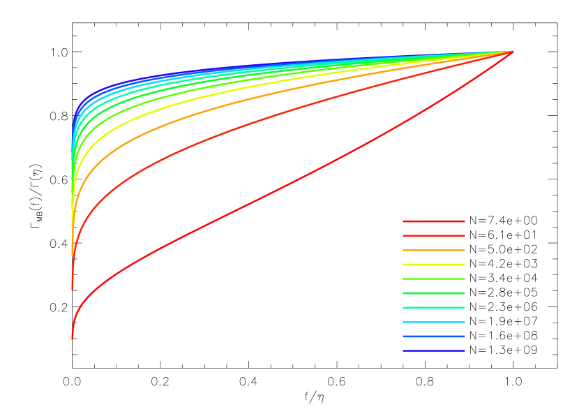
Figure 1: The behavior of the relaxation function $\Gamma_{\rm MB}$ as a function of the coarse-grained distribution function $f$ in a system that obeys Maxwell-Boltzmann statistics. The various lines represent functions defined with different $N$ values, where $N$ is basically the number of particles in a system. As $N$ increases, the relaxation function becomes more constant.

where the value of the fine-grained distribution function $\eta$ is the maximum value allowed for $f$. In a collisional system that follows the Maxwell-Boltzmann distribution, like an ordinary gas, one could imagine $f$ reaching any value due to collisions. However, for the collisionless case, MB statistics are the non-degenerate limit, implying that $f\ll\eta$. Figure 1 contains plots of $\Gamma_{\rm MB}(f)$ for a variety of values of $N$. As $N$ increases, the relaxation function becomes more and more uniform.

3.2 Lynden-Bell Statistics

We now investigate a system that obeys Lynden-Bell statistics. The entropy of the system can be transformed from the summation in Equation 10 to,

$$S_{\rm LB}=-k_{\rm B}\iint f\left[\ln{\left(\frac{\nu}{\eta}f\right)}-\frac{S_{0}}{Nk_{\rm B}}\right]+(\eta-f)\ln{\left(\frac{\nu}{\eta}(\eta-f)\right)}\>\mathrm{d}\boldsymbol{x}\mathrm{d}\boldsymbol{v},$$ (29)

where $S_{0}=Nk_{\rm B}(\ln{N}-1)+k_{\rm B}\sum_{i}\nu\ln{\nu}$. The entropy density can now be written as,

$$\rho s_{\rm LB}=-k_{\rm B}\int f\left[\ln{\left(\frac{\nu}{\eta}f\right)}-\frac{S_{0}}{Nk_{\rm B}}\right]+(\eta-f)\ln{\left(\frac{\nu}{\eta}(\eta-f)\right)}\>\mathrm{d}\boldsymbol{v}.$$ (30)

Taking a partial time derivative of Equation 30 results in

$$\frac{\partial}{\partial t}(\rho s_{\rm LB}) = -k_{\rm B}\int\frac{\partial f}{\partial t}\left[\ln{\left(\frac{f}{\eta-f}\right)}-C\right]\>\mathrm{d}\boldsymbol{v}$$ (31)

$$= -k_{\rm B}\int\frac{\partial f}{\partial t}\ln{\left(\frac{f}{\eta-f}\right)}\>\mathrm{d}\boldsymbol{v}+k_{\rm B}C\int\frac{\partial f}{\partial t}\>\mathrm{d}\boldsymbol{v},$$

where $C=S_{0}/Nk_{\rm B}$ is a constant.

Substituting $\partial f/\partial t$ from the Boltzmann equation into Equation 31 again results in a lengthy expression that we will deal with term by term. For reference, the expression after substitution is,

$$\frac{\partial}{\partial t}(\rho s_{\rm LB})=$$ (32)

$$-k_{\rm B}\int(-\boldsymbol{v}\boldsymbol{\cdot}\boldsymbol{\nabla}f)\ln{\left(\frac{f}{\eta-f}\right)}\>\mathrm{d}\boldsymbol{v}-k_{\rm B}\int(-\boldsymbol{a}\boldsymbol{\cdot}\boldsymbol{\nabla}_{v}f)\ln{\left(\frac{f}{\eta-f}\right)}\>\mathrm{d}\boldsymbol{v}-$$

$$k_{\rm B}\int\Gamma\ln{\left(\frac{f}{\eta-f}\right)}\>\mathrm{d}\boldsymbol{v}+k_{\rm B}\int(-\boldsymbol{v}\boldsymbol{\cdot}\boldsymbol{\nabla}f)C\>\mathrm{d}\boldsymbol{v}+k_{\rm B}\int(-\boldsymbol{a}\boldsymbol{\cdot}\boldsymbol{\nabla}_{v}f)C\>\mathrm{d}\boldsymbol{v}+$$

$$k_{\rm B}\int\Gamma C\>\mathrm{d}\boldsymbol{v}.$$

The first integral on the right-hand side of Equation 32 can be transformed to,

$$\int(\boldsymbol{v}\boldsymbol{\cdot}\boldsymbol{\nabla}f)\ln{\left(\frac{f}{\eta-f}\right)}\>\mathrm{d}\boldsymbol{v}=\boldsymbol{\nabla}\boldsymbol{\cdot}\int f\ln{\left(\frac{f}{\eta-f}\right)}\boldsymbol{v}\>\mathrm{d}\boldsymbol{v}-\int\frac{\eta}{\eta-f}\boldsymbol{v}\boldsymbol{\cdot}\boldsymbol{\nabla}f\>\mathrm{d}\boldsymbol{v}.$$ (33)

We now re-write the first term on the right-hand side of Equation 33 as,

$$\boldsymbol{\nabla}\boldsymbol{\cdot}\int f\ln{\left(\frac{f}{\eta-f}\right)}\boldsymbol{v}\>\mathrm{d}\boldsymbol{v}=\boldsymbol{\nabla}\boldsymbol{\cdot}\int f\left[\ln{\left(\frac{\nu}{\eta}f\right)}-\ln{\left(\frac{\nu}{\eta}(\eta-f)\right)}\right]\boldsymbol{v}\>\mathrm{d}\boldsymbol{v}.$$ (34)

Adding and subtracting terms of the form $\boldsymbol{\nabla}\boldsymbol{\cdot}\int\eta\ln{[(\nu/\eta)(\eta-f)]}\boldsymbol{v}\>\mathrm{d}\boldsymbol{v}$ to Equation 34 gives us a term that is very reminiscent of the entropy density in Equation 30,

$$\int(\boldsymbol{v}\boldsymbol{\cdot}\boldsymbol{\nabla}f)\ln{\left(\frac{f}{\eta-f}\right)}\>\mathrm{d}\boldsymbol{v}=$$ (35)

$$\boldsymbol{\nabla}\boldsymbol{\cdot}\int\left[f\ln{\left(\frac{\nu}{\eta}f\right)}+(\eta-f)\ln{\left(\frac{\nu}{\eta}(\eta-f)\right)}\right]\boldsymbol{v}\>\mathrm{d}\boldsymbol{v}-$$

$$\boldsymbol{\nabla}\boldsymbol{\cdot}\int\eta\ln{\left(\frac{\nu}{\eta}(\eta-f)\right)}\boldsymbol{v}\>\mathrm{d}\boldsymbol{v}-\int\frac{\eta}{\eta-f}\boldsymbol{v}\boldsymbol{\cdot}\boldsymbol{\nabla}f\>\mathrm{d}\boldsymbol{v}.$$

Looking at the second term on the right-hand side of Equation 35, we see that

$$\boldsymbol{\nabla}\boldsymbol{\cdot}\eta\ln{\left(\frac{\nu}{\eta}(\eta-f)\right)}\boldsymbol{v}=-\frac{\eta}{\eta-f}\boldsymbol{v}\boldsymbol{\cdot}\boldsymbol{\nabla}f.$$ (36)

We can now simplify Equation 35 to

$$\int(\boldsymbol{v}\boldsymbol{\cdot}\boldsymbol{\nabla}f)\ln{\left(\frac{f}{\eta-f}\right)}\>\mathrm{d}\boldsymbol{v}=\boldsymbol{\nabla}\boldsymbol{\cdot}\int\left[f\ln{\left(\frac{\nu}{\eta}f\right)}+(\eta-f)\ln{\left(\frac{\nu}{\eta}(\eta-f)\right)}\right]\boldsymbol{v}\>\mathrm{d}\boldsymbol{v}.$$ (37)

Next, we deal with the second integral on the right-hand side of Equation 32. Since $\boldsymbol{a}$ is velocity-independent, we can write

$$\int(\boldsymbol{a}\boldsymbol{\cdot}\boldsymbol{\nabla}_{v}f)\ln{\left(\frac{f}{\eta-f}\right)}\>\mathrm{d}\boldsymbol{v}=\boldsymbol{a}\boldsymbol{\cdot}\int(\boldsymbol{\nabla}_{v}f)\ln{\left(\frac{f}{\eta-f}\right)}\>\mathrm{d}\boldsymbol{v}.$$ (38)

Using

$$(\boldsymbol{\nabla}_{v}f)\ln{\left(\frac{f}{\eta-f}\right)}=\boldsymbol{\nabla}_{v}\left[f\ln{\left(\frac{f}{\eta-f}\right)}\right]-\frac{\eta}{\eta-f}\boldsymbol{\nabla}_{v}f,$$ (39)

and taking advantage of the velocity independence of $\boldsymbol{a}$, we can re-write the right-hand side of Equation 38 as,

$$\int\boldsymbol{\nabla}_{v}\boldsymbol{\cdot}\left[\boldsymbol{a}f\ln{\left(\frac{f}{\eta-f}\right)}\right]\>\mathrm{d}\boldsymbol{v}-\int\frac{\eta}{\eta-f}\boldsymbol{a}\boldsymbol{\cdot}\boldsymbol{\nabla}_{v}f\>\mathrm{d}\boldsymbol{v}.$$ (40)

The first term disappears when the divergence theorem is applied, as the distribution function goes to zero at large velocities. To deal with the second term, we substitute $\boldsymbol{\nabla}_{v}f=-\boldsymbol{\nabla}_{v}(\eta-f)$ to get,

$$-\int\frac{\eta}{\eta-f}\boldsymbol{a}\boldsymbol{\cdot}\boldsymbol{\nabla}_{v}f\>\mathrm{d}\boldsymbol{v}=\eta\boldsymbol{a}\boldsymbol{\cdot}\int\boldsymbol{\nabla}_{v}\ln{(\eta-f)}\>\mathrm{d}\boldsymbol{v}.$$ (41)

Let us investigate one component of this vector integral,

$$\int_{-\infty}^{\infty}\frac{\partial}{\partial v_{x}}\ln{(\eta-f)}\>\mathrm{d}v_{x}=\ln{(\eta-f)}\big{|}_{-v_{\rm max}}^{v_{\rm max}}=\ln{\eta}-\ln{\eta}=0,$$ (42)

since a well-behaved distribution function is expected to disappear at the largest speeds possible. So, the second integral on the right-hand side of Equation 32 is zero.

We now re-combine the terms on the right-hand side of Equation 32 using the results of Equations 37 and 38 to produce our final representation of the time rate of change of the entropy density,

$$\frac{\partial}{\partial t}(\rho s_{\rm LB})=$$ (43)

$$-k_{\rm B}\boldsymbol{\nabla}\boldsymbol{\cdot}\int\left\{f\left[\ln{\left(\frac{f}{\eta-f}\right)}-C\right]+(\eta-f)\ln{\left(\frac{\nu}{\eta}(\eta-f)\right)}\right\}\boldsymbol{v}\>\mathrm{d}\boldsymbol{v}-$$

$$k_{\rm B}\int\Gamma\left[\ln{\left(\frac{f}{\eta-f}\right)}-C\right]\>\mathrm{d}\boldsymbol{v}.$$

Again assuming the velocity field to be composed of mean and peculiar components $\boldsymbol{v}=\boldsymbol{v_{0}}+\boldsymbol{v_{p}}$, we draw a correspondence between,

$$\frac{\partial}{\partial t}(\rho s_{\rm LB})=-\boldsymbol{\nabla}\boldsymbol{\cdot}\rho s_{\rm LB}\boldsymbol{v_{0}}-$$ (44)

$$k_{\rm B}\boldsymbol{\nabla}\boldsymbol{\cdot}\int\left\{f\left[\ln{\left(\frac{f}{\eta-f}\right)}-C\right]+(\eta-f)\ln{\left(\frac{\nu}{\eta}(\eta-f)\right)}\right\}\boldsymbol{v_{p}}\>\mathrm{d}\boldsymbol{v}-$$

$$k_{\rm B}\int\Gamma\left[\ln{\left(\frac{f}{\eta-f}\right)}-C\right]\>\mathrm{d}\boldsymbol{v},$$

and Equation 6

$$\frac{\partial}{\partial t}(\rho s)=-\boldsymbol{\nabla}\boldsymbol{\cdot}(\boldsymbol{\Sigma}+\rho s\boldsymbol{v_{0}})+\sigma.$$ (45)

The entropy flux due to random motions $\boldsymbol{\Sigma}$ is given by the integral in the second term on the right-hand side of Equation 44. The remaining term then makes up the entropy production for the system,

$$\sigma_{\rm LB}=-k_{\rm B}\int\Gamma\left[\ln{\left(\frac{f}{\eta-f}\right)}-C\right]\>\mathrm{d}\boldsymbol{v}.$$ (46)

Again, there is a relaxation function-dependent term in the entropy production. Following the same steps as in the Maxwell-Boltzmann case, we find that the condition for the entropy production term in Equation 46 to be extremized is,

$$\Gamma_{\rm LB}(f)=\frac{Q}{\ln{[f/(\eta-f)]}-C},$$ (47)

where $Q$ is an integration constant and $C=\ln{N}-1+1/N\sum_{i}\nu\ln{\nu}$. If we set $f=\eta/2$, $Q=-C\Gamma_{\rm LB}(f=\eta/2)$ and

$$\Gamma_{\rm LB}(f)=\frac{-C\Gamma_{\rm LB}(f=\eta/2)}{\ln{[f/(\eta-f)]}-C}.$$ (48)

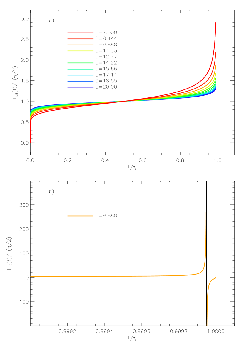
Figure 2: a) The behavior of the relaxation function $\Gamma_{\rm LB}$ as a function of the coarse-grained distribution function $f$ in a system that obeys Lynden-Bell statistics. The various lines represent functions defined with different $C$ values, where $C=\ln{N}-1+1/N\sum_{i}\nu\ln{\nu}$. As before, $N$ is basically the number of particles in a system, and increasing $N$ results in increasing $C$. Like the Maxwell-Boltzmann case, as $N$ increases, the relaxation function becomes more constant. b) A magnified view of the behavior of $\Gamma_{\rm LB}$ (for a fixed $C$) as $f\rightarrow\eta$. Note that $\Gamma_{\rm LB}$ becomes unbound as $\ln{[f/(\eta-f)]}\rightarrow C$, but as $f\rightarrow\eta$, $\Gamma_{\rm LB}\rightarrow 0$.

Like $\Gamma_{\rm MB}$, this function behaves more like a constant as the $N$ value increases ($C\rightarrow\infty$). $\Gamma_{\rm LB}$ curves for a variety of $C$ values are presented in Figure 2a. The increase in $\Gamma_{\rm LB}$ seen as $f/\eta\rightarrow 1$ is due to $\ln{[f/(\eta-f)]}$ approaching $C$. Once $f$ is sufficiently close to $\eta$ that subtracting $C$ produces a negligible change, $\Gamma_{\rm LB}\rightarrow 0$. The complex behavior of $\Gamma_{\rm LB}$ for $f\approx\eta$ is shown in Figure 2b and is discussed further in the next section.

4 Discussion & Conclusions

The seminal paper by Lynden-Bell (1967) has shown that, under certain assumptions, there is no maximum entropy state for self-gravitating systems. Alternative descriptions of the same systems which yield self-consistent results under entropy extremization may be found in Madsen (1996) and Hjorth & Williams (2010).

Lynden-Bell’s conclusion is exemplified by the order-of-magnitude calculation in Tremaine, Hénon, & Lynden-Bell (1986, S. 4.7); Binney & Tremaine (1987, S. 4.7), using Maxwell-Boltzmann statistics. The result of this calculation is that when a collisionless system rearranges its mass to become more centrally concentrated in the core, the entropy of the contracting core mass decreases. The outer envelope, expanding in response to the contracting core to satisfy the virial theorem, should have an increase in entropy. As a result, the entropy for the entire system increases. Since a system can always increase its entropy by contracting the core and expanding the envelope, there is no maximum entropy state, and hence maximizing entropy will not lead to a satisfactory description of a steady state.

Yet, we know from numerous high-resolution $N$-body simulations that long-lived steady states do exist. How does one find these theoretically? Apparently, one has to resort to means other other than entropy extremization. In this paper we try one alternative approach. We apply a principle of extremizing entropy production rate to self-gravitating systems. This principle has been used widely to describe thermal non-equilibrium, but not in systems that are self-gravitating.

Our basic hypothesis is that a steady state is obtained by extremizing the entropy production. We present expressions for the entropy production rates for two types of statistics, Maxwell-Boltzmann (MB) and Lynden-Bell (LB), as Equations 24 and 46, respectively. We then find expressions (Equations 28 and 48) for the relaxation term that forms the right hand side of the coarse-grained Boltzmann equation. The meaning of these expressions and the interpretation of our results, under the assumption that this idea is applicable to self-gravitating systems, are discussed below.

4.1 Entropy production

The development of the expressions for entropy production rates $\sigma$ is a central result of this work. The descriptions of $\sigma$ for the MB and LB statistical families are given in Equations 24 and 46, respectively. Since we are dealing with collisionless systems exclusively, one might expect these to be zero. In fact, if we were considering the fine-grained distribution function, there would be no entropy change, no thermodynamic evolution, as the collisionless $\mathrm{d}f/\mathrm{d}t=0$ Boltzmann equation would apply.

However, we are considering the coarse-grained function. As a system evolves, the fine-grained distribution function becomes stretched and twisted in phase-space. Because the coarse-grained function averages the fine-grained function with nearby empty regions of phase-space, the coarse-grained function changes as the system evolves. Now, recall that entropy represents the number of accessible states. On the level of the fine-grained function, the number of accessible states stays the same. However, going from a fine-grained to coarse-grained description implies that there are now regions of phase-space not occupied by the fine-grained function that are accessible to the coarse-grained function. This implies that there are more microscopic ways of realizing a given macroscopic state, leading to more possible states and larger entropy. Thus, coarse-graining an evolving system results in entropy production even in a collisionless system. In terms of physical processes, the evolution is due to the larger-scale phase-space evolution of the system driven by collisionless relaxation processes, like violent relaxation and phase mixing.

The above argues that entropy production takes places during evolution of collisionless systems. But our analysis shows that entropy production takes place even during the steady state. Let us start by writing down the expression for the entropy production during the steady-state by combining Equations 24 and 28 for the MB case,

$$\sigma_{\rm MB} = -k_{\rm B}\int Q\Gamma_{\rm MB}(\eta)\>\mathrm{d}\boldsymbol{v}$$ (49)

$$= -k_{\rm B}Q\Gamma_{\rm MB}(f=\eta)V_{\rm velocity},$$

where $V_{\rm velocity}$ is the volume of occupied velocity space. This is consistent with the second law of thermodynamics since $Q<0$ and all other terms are positive. A similar expression can be found for the LB case, using Equations 46 and 48. Since a steady state is described by an unchanging value of $\sigma$, any non-zero value of $\sigma$ persists even when a system has reached mechanical equilibrium.

It is interesting to think of the source of this continued entropy production. After a system stops evolving on the macroscopic scale, it still continues to evolve on ever decreasing microscopic scales as the fine-grained function continues to stretch and twist almost indefinitely. The corresponding continual coarse-graining of the ever evolving fine-grained function on smaller and smaller scales, results in constant, non-zero entropy production.

4.2 Interpreting the Boltzmann Equation

Our expression for the Boltzmann equation states that the relaxation function, $\Gamma$, determines the rate of change of the coarse-grained distribution function,

$$\frac{\mathrm{d}f}{\mathrm{d}t}=\Gamma(f).$$ (50)

Despite the right hand side being non-zero (given by Equations 28 and 48 for the MB and LB statistics, respectively), the above equation does not contradict the assumption of a stationary state. A stationary, or steady, state is the Eulerian viewpoint, i.e., $\partial f/\partial t=0$, while the Boltzmann equation above is a Lagrangian viewpoint. $\partial f/\partial t=0$ does not imply $\mathrm{d}f/\mathrm{d}t=0$. In other words, the relaxation function $\Gamma$ does not determine the explicit time-dependence of $f$, which must be zero for stationary states, but rather describes a flux of occupied cells through phase-space, as do the velocity-driven ($\boldsymbol{v}\boldsymbol{\cdot}\boldsymbol{\nabla}f$) and acceleration-driven ($\boldsymbol{a}\boldsymbol{\cdot}\boldsymbol{\nabla}_{v}f$) flux terms (c.f. Equation 13). In the context of the Lagrangian derivative, we can think of $t$ simply as a parameter that indicates the location along a particle’s or cell’s path through phase-space.

In collisional systems, the relaxation function is called the collision term and is usually dealt with in a Fokker-Planck approximation scheme. In these systems the particles, through two-body encounters, gradually disperse over the whole available phase-space, and so $\mathrm{d}f/\mathrm{d}t$ following any given particle in an evolving system does not stay constant, but generally decreases with time. In a general collisionless system, this term represents the processes like violent relaxation and phase mixing, on the coarse-grained scale. In a steady-state collisionless system, the large scale processes like violent relaxation no longer operate and the only changes happen on microscopic scales. In this context, the left hand side of Equation 50 describes how a particle, or a cell moves through the system (and $t$ is the parameter). Therefore it is not unexpected that over some portions of its motion the coarse-grained density around it will be increasing and over others, it will be decreasing. For the MB case, $\Gamma_{\rm MB}>0$ for $f>0$, implying that $f$ should continually grow. However, this is impossible as the coarse-grained distribution function is limited to a maximum value $\eta$. This contradiction arises as MB statistics are valid only when $f\ll\eta$ so that macro-cells are not multiply occupied. On the other hand, the LB case does not present any contradictions with the Boltzmann equation. $\Gamma_{\rm LB}$ is zero when $f=0$ and $f=\eta$, and is positive over the vast majority of the intervening range. This behavior guarantees that when the coarse-grained density reaches its maximum value, the relaxation term disappears and the system behaves collisionlessly even at the coarse-grained level.

To sum up, if extremizing entropy production in self-gravitating systems does lead to steady-state configurations, then Equation 50 with the appropriate expressions for $\Gamma$ (as given by Equations 28 and 48) describes the steady state of self-gravitating collisionless systems. The relaxation term $\Gamma$ describes the continual evolution of the coarse-grained distribution function, which is due to the combimation of the dynamical evolution of the fine-grained DF on microscopic scales, and coarse-graining.

References

- Binney & Tremaine (1987) Binney, J., Tremaine, S. 1987, Galactic Dynamics, (Princeton, NJ:Princeton)
- Bordel (2010) Bordel, S. 2010, Physica A, 389, 4564
- de Groot & Mazur (1984) de Groot, S. R., Mazur, P. 1984, Non-Equilibrium Thermodynamics, (Mineola, NY:Dover)
- Grandy (2008) Grandy, W. T. 2008, Entropy and the Time Evolution of Macroscopic Systems, (New York, NY:Oxford)
- Hjorth & Williams (2010) Hjorth, J., Williams, L. L. R. 2010, ApJ, 722, 851
- Kandrup (1998) Kandrup, H. E. 1998, ApJ, 500, 120
- Lynden-Bell (1967) Lynden-Bell, D. 1967, MNRAS, 136, 101
- Madsen (1996) Madsen, J. 1996, MNRAS, 280, 1089
- Martyushev & Seleznev (2006) Martyushev, L. M., Seleznev, V. D. 2006, Phys. Rep. 426, 1
- Merritt & Aguilar (1985) Merritt, D., Aguilar, L. 1985, MNRAS, 217, 787
- Moore et al. (1998) Moore, B., Governato, F., Quinn, T., Stadel, J., Lake, G. 1998, ApJ, 499, L5
- Navarro, Frenk, & White (1996) Navarro, J. F., Frenk, C. S., White, S. D. M. 1996, ApJ, 462, 563
- Plastino & Plastino (1993) Plastino, A. R., Plastino, A. 1993, Phys. Lett. A, 174, 384
- Prigogine (1978) Prigogine, I. 1978, Science 201, 777
- Prigogine & Geheniau (1986) Prigogine. I., Geheniau, J. 1986, Proc. Natl. Acad. Sci. USA, 83, 6245
- Taylor & Navarro (2001) Taylor, J. E., Navarro, J. F. 2001, ApJ, 563, 483
- Tremaine, Hénon, & Lynden-Bell (1986) Tremaine, S., Hénon, M., Lynden-Bell, D. 1986, MNRAS, 219, 285
- Tsallis (1988) Tsallis, C. 1988, J. Stat. Phys., 52, 479
- van Albada (1982) van Albada, T. S. 1982, MNRAS, 201, 939
- Ziegler (1961) Ziegler, H. 1961, Ing. Arch. 30, 410