QSO Selection Algorithm Using Time Variability and Machine Learning:
Selection of 1,620 QSO Candidates from MACHO LMC Database

Abstract

We present a new QSO selection algorithm using a Support Vector Machine (SVM), a supervised classification method, on a set of extracted time series features including period, amplitude, color, and autocorrelation value. We train a model that separates QSOs from variable stars, non-variable stars and microlensing events using 58 known QSOs, 1,629 variable stars and 4,288 non-variables using the MAssive Compact Halo Object (MACHO) database as a training set. To estimate the efficiency and the accuracy of the model, we perform a cross-validation test using the training set. The test shows that the model correctly identifies $\sim$80% of known QSOs with a 25% false positive rate. The majority of the false positives are Be stars.

We applied the trained model to the MACHO Large Magellanic Cloud (LMC) dataset, which consists of 40 million lightcurves, and found 1,620 QSO candidates. During the selection none of the 33,242 known MACHO variables were misclassified as QSO candidates. In order to estimate the true false positive rate, we crossmatched the candidates with astronomical catalogs including the Spitzer Surveying the Agents of a Galaxy’s Evolution (SAGE) LMC catalog and a few X-ray catalogs. The results further suggest that the majority of the candidates, more than 70%, are QSOs.

1. Introduction

A large catalog of Quasi-stellar object (QSO) is important for a variety of fields in modern astrophysics and observational cosmology. QSOs have been used for studies of a) large scale structures based on the spatial clustering of QSOs (Shen et al., 2007; Ross et al., 2009), b) growth of central black holes using the estimated black holes’ masses (Kollmeier et al., 2006), c) coevolution of black holes and their host galaxies using lensed QSO hosts (Peng et al., 2006), d) the epoch of reionization based on high redshift QSOs (Becker et al., 2001; Fan et al., 2006), e) dark matter substructure using gravitationally lensed QSOs (Metcalf & Madau, 2001; Miranda & Macciò, 2007) and f) properties of the intergalactic medium determined by measuring metallicity distribution using QSO spectra (Viel et al., 2002; Simcoe et al., 2004).

One of the most interesting properties of QSOs is the strong flux variation over a wide range of wavelengths on timescales from days to years (Hook et al. 1994; Hawkins 2002 and references therein). It is believed that QSO variability is associated with accretion disk instabilities (Rees, 1984; Kawaguchi et al., 1998) although there are other possible explanations for the source of QSO variability, including microlensing (Hawkins, 1993; Zackrisson et al., 2003), starbursts and supernovae (Terlevich et al., 1992; Aretxaga et al., 1997). It is debatable which mechanism is the dominant source of variability (see Hook et al. 1994; Giveon et al. 1999; Vanden Berk et al. 2004; de Vries et al. 2005; Bauer et al. 2009). Moreover, due to the lack of long-time-span, well-sampled and high-quality QSO lightcurves, all these previous studies have investigated ensemble variabilities of QSOs. Thus it is important to have a large set of well-sampled QSO lightcurves in order to study both ensemble and individual QSO variability characteristics, which will help constrain the theoretical models of the variability mechanisms (see Hook et al. 1994; Cristiani et al. 1996; Vanden Berk et al. 2004 and references therein).

Many authors have attempted to select QSO candidates based on the variability characteristics. For instance, Eyer (2002) selected QSO candidates from 68,000 OGLE-II variable stars (Zebrun et al., 2001) using colors, magnitudes and the structure function of the variables. The structure function determines the time scale of variability in a given lightcurve as a function of the time lag between observations (Eyer, 2002). Among the selected 133 QSO candidates, $\sim$10% were confirmed to be QSOs (Dobrzycki et al., 2002, 2005). Geha et al. (2003) (hereinafter G03) searched 140,000 MACHO sources that have significant flux variation (Alcock et al., 2000). G03 used colors, magnitudes and two statistical parameters that quantify variability to select QSO candidates. G03 then removed known MACHO variable stars (Alcock et al., 2001) from the candidate list and finally examined the remaining candidates manually in order to remove false positives. Among the final 360 candidates, 259 were spectroscopically observed and 47 of them confirmed to be QSOs. Sumi et al. (2005) searched about 200,000 variable objects of the OGLE-II data (Wozniak et al., 2002) and then used a few selection cuts such as magnitudes, structure function and manual validation. No spectroscopic observation was done for their final 97 QSO candidates.

Recently, four QSO selection methods have been submitted or published, which proposed new QSO classification algorithms using time series variability features. One of them is the work done by Kozłowski et al. (2010) that used a stochastic model shown in Kelly et al. (2009) which derives the amplitude and the time scale of lightcurve variations. They also employed periods of lightcurves and magnitudes. To develop their selection method, they used the known QSOs, periodic variables and non-periodic variables in the OGLE databases (Udalski et al., 1997, 2008). They also used QSO candidates from Kozłowski & Kochanek (2009) that had OGLE counterparts. To separate the QSOs from other variables, they defined several cuts and correctly identified 63% of the QSOs while removing most of the variable stars. The second study (Schmidt et al., 2010) proposed a power-law model to fit the structure function and derived the amplitude and the power index of the model. They used the derived parameters to isolate known QSOs from RR Lyraes and non-variable stars extracted from the SDSS stripe 82 database (S82) (Sesar et al., 2007). Using simple cuts on the amplitude versus power index plane, they identified about 90% of the SDSS QSOs with a 5% false positive rate. Butler & Bloom (2010) and MacLeod et al. (2010) used similar approaches (i.e. structure function) with the previous two works. Both utilized the preselected variable sources from the S82 dataset where the majority of the variables are QSOs, RR Lyraes and stars from the stellar locus (see Sesar et al. 2007 for details). Butler & Bloom (2010) parameterized the ensemble QSO structure function as a function of brightness of the QSOs. They then used the parameterized ensemble QSO model to evaluate the quasar likelihood for individual lightcurves (see Butler & Bloom 2010 for details). Using this method, they identified nearly all the known SDSS QSOs (99%) with a 3% false positive rate. MacLeod et al. (2010) also used the structure function and several cuts to identify QSOs and exclude other variable stars from the S82 database. They correctly selected about 90% of the QSOs with 10$\sim$20% false positive rate depending on the cuts imposed. Both works also selected new QSO candidates from the preselected variable sources (Sesar et al., 2007). These candidates have not been spectroscopically confirmed. Note that the efficiencies or false positive rates of these studies should not be directly compared because each work used their own selected set of stars and QSOs to develop their methods. For a comprehensive comparison of the results of the methods, see MacLeod et al. (2010).

Even though some of these recent works (Schmidt et al., 2010; Butler & Bloom, 2010; MacLeod et al., 2010) showed high efficiencies and low false positive rates, they used samples that are selected in such a way that high efficiency and low false positive rate is to be expected. The separation of QSOs from non-varying stars and a few types of variable stars, especially short-period variables (i.e. RR Lyraes) are relatively straightforward since QSOs show non-periodic and long-time scale fluctuation. The majority of the samples they used in these studies are short-period variables and do not show long-time scale fluctuation,

QSO selection methods based on variability will be valuable tools for on-going and future large scale survey missions such as Pan-STARRS (Kaiser, 2004) and LSST (Ivezic et al., 2008). These surveys will keep monitoring wide areas of the sky and will produce vast amount of time series data in several wavelength bands (e.g. $g,r,i,z$ for Pan-STARRS). Because spectroscopic observations for such wide areas are very expensive, QSO selections in the absence of spectroscopic data are becoming important, and thus developing QSO selection methods using variability are rapidly attracting notable attention.

The work presented in this paper utilizes the whole MACHO lightcurve databset considering all known variable sources in the MACHO database. Thus this is the first work that considers the efficiency and the false positive rates of QSO selection in an entire lightcurve dataset. We have developed our method by training on the richest possible dataset including all known types of sources and testing it also on the whole dataset. The training set includes a variety of variable objects such as QSOs, RR Lyraes, Cepheids, eclipsing binaries, long period variables, Be stars, microlensing events and also non-variable stars. Only one other selection method, Kozłowski et al. (2010), has considered Be stars, which are one of the most significant contaminants during QSO selections in LMC (G03). Our goal is to select high confidence QSO candidates in the MACHO database (Alcock et al., 1996) while minimizing the number of false positives. Our approach employs multiple time series features rather than using only the lightcurve structure function. These features can characterize various kinds of variability characteristics. Therefore our algorithm is practical not only for identifying QSOs but also for excluding other types of variable stars and non-variable stars. To fully utilize the features and identify QSOs, we employed a supervised machine learning classification method, Support Vector Machine (SVM, Boser et al. 1992; Cristianini & Shawe-Taylor 2000; Panik 2005). In the true spirit of machine learning, our method uses a classification model trained with the training set and thus eliminates the need for hard linear cuts and human input (e.g. manual preselection of variable sets, manual removal of false positives and determination of cuts).

We briefly introduce the MACHO database and known MACHO QSOs in Section 2. Section Appendix describes the multiple time series features that we used to quantify the variability characteristics of each lightcurve. Section 4 introduces SVM, the method used to train the classification model. We present the MACHO QSO classification model constructed using the time series features and SVM in Section 5.1. We then show the MACHO QSO candidates selected using the model in Section 5.2. Crossmatched results with astronomical catalogs are presented in Section 6. Ongoing and future work is summarized in Section 7.

Table 111 time series features

Four new features	Brief description; for details, see Appendix.
$N_{above}$ and $N_{below}$	$N_{above}$: the number of points above the upper boundary line of the autocorrelation plot.
	$N_{below}$: the number of points below the lower boundary line of the autocorrelation plot.
	Figure 11 shows the constructed boundary lines based on the autocorrelation functions (see Figure 10)
	of the training set lightcurves.
Stetson $K_{AC}$	Stetson $K$ (Eq. 23) variability index derived based on the autocorrelation function
	of each lightcurve.
$R_{cs}$	The range of a cumulative sum (Ellaway, 1978).
Seven other features	Brief description; for details, see Appendix.
$\sigma/\bar{m}$	The ratio of the standard deviation, $\sigma$, to the mean magnitude, $\bar{m}$.
Period and Period S/N	Period and period signal-to-noise ratio of each lightcurve.
	Derived using Lomb-Scargle algorithm and Lomb periodogram (Lomb, 1976; Scargle, 1982).
Stetson $L$	The variability index (Stetson, 1996) describes the synchronous variability of different bands.
$\eta$	The ratio of the mean of the square of successive differences to the variance of data points
	in each lightcurve.
$B-R$	The average color for each lightcurve.
$Con$	The number of consecutive data points that are brighter or fainter than 2$\sigma$ of each lightcurve.

2. MACHO database and MACHO QSO

2.1. MACHO database

The MACHO survey monitored a wide area of the sky to detect microlensing events caused by Milky Way halo objects and test the hypothesis that a significant portion of dark matter in the Milky Way halo consists of compact objects such as brown dwarfs or planets (Alcock et al., 1996). Because microlensing events are extremely rare, MACHO monitored several tens of millions of stars in the Large Magellanic Cloud (LMC), Small Magellanic Cloud (SMC) and Galactic bulge for 7.4 years. Observations started in July 1992 and were completed at the end of December 1999. More than 5 Tbytes of image data and 70,000 exposures were collected during the period (Alcock et al., 2000). In addition, MACHO used two bands (MACHO B and R) for the observations.

2.2. MACHO QSOs

There are in total 59 known QSOs in the MACHO database (50 in the LMC fields and 9 in the SMC fields; hereinafter MACHO QSOs). Forty-seven were detected by G03 and the remaining twelve were QSOs previously known from other studies (Blanco & Heathcote, 1986; Schmidtke et al., 1999; Dobrzycki et al., 2002). G03 detected 38 of them using variability characteristics of MACHO lightcurves and nine of them by crossmatching with X-ray and radio catalogs. To select QSO candidates, G03 applied simple cuts such as color, magnitude and amplitude on 140,000 preselected MACHO sources that show strong flux variation (Alcock et al., 2000). The lightcurves of 12 previously known QSOs were used as references for the variability cuts. After selecting 2,500 QSO candidates from the 140,000 sources, G03 removed known MACHO variable stars from the candidate list and then manually examined the remaining candidates to eliminate false positives. They eventually removed about 2,140 candidates and confirmed that the majority of the removed candidates were objects with quasi-periodic variability such as blue variable stars. Blue variable stars typically show strong Balmer emission lines and are thought to be associated with Be stars (Keller et al., 2002). It is also known that Be stars show variability similar to QSOs (Eyer, 2002; Geha et al., 2003; Mennickent et al., 2002; Keller et al., 2002). Using spectroscopic instruments, G03 observed 259 candidates selected from the remaining 360 candidates and also the candidates selected using the catalog crossmatchings. G03 confirmed 47 new QSOs with magnitudes $16.63<m_{V}<20.10$ and redshifts between 0.28 and 2.77.

G03 analyzed only 30 of the 82 MACHO LMC fields, and thus the remaining 52 MACHO LMC fields have not been searched for QSOs. Moreover, they selected QSO candidates from the preselected 140,000 variable sources and did not analyze the remaining several tens of million lightcurves. Thus it is very likely that there are a lot more QSOs that have not been detected yet. In the following sections, we introduce a new QSO selection algorithm to detect these non-identified QSOs in the MACHO LMC database.

3. Time Series Features

In order to separate QSOs from non-variable stars and variable stars, we quantify the variability characteristics of lightcurves using 11 time series features. These 11 features were independently proposed to quantify certain types of variability features including amplitudes, periods, colors and distribution of data points. They can complement each other because they pick out different variability features. Thus, by using these multiple features, we can identify various types of variability characteristics (e.g. non-varying sources, periodic variables and non-periodic variables). Note that we selected these time series features not only for characterizing QSO time series but also for characterizing other types of variable sources or non-variable sources because we want to identify QSOs while excluding the other types of sources at the same time. We briefly describe these 11 time series features in Table 1. See Appendix for details about the features consisting of four new features that we have developed for this work and seven previously used features.

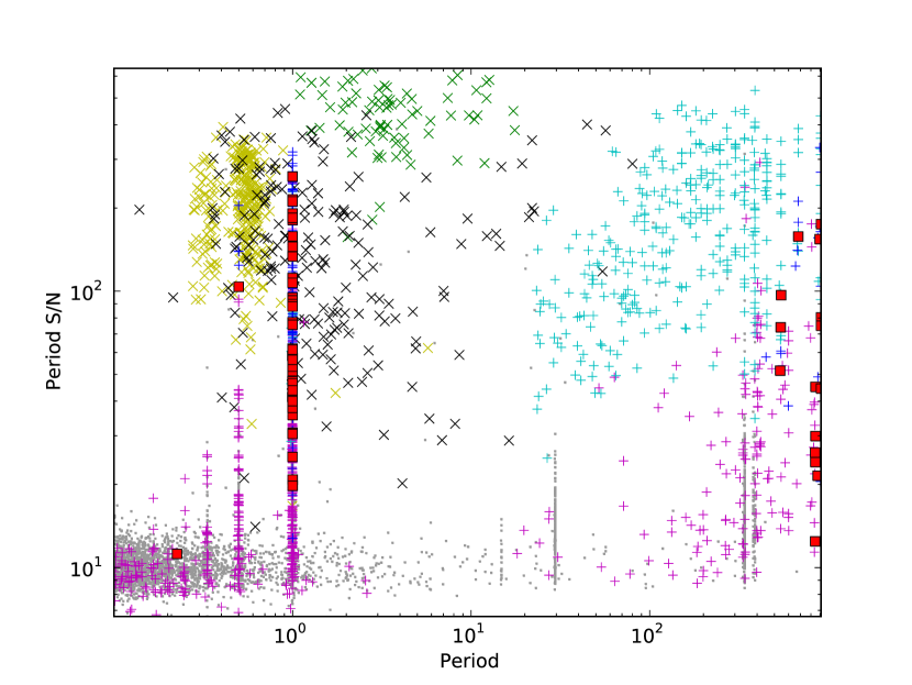
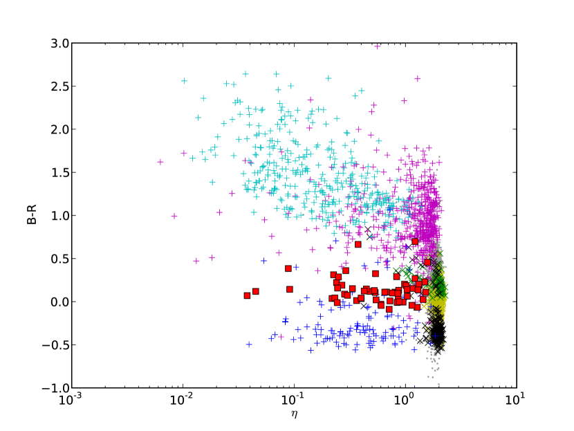
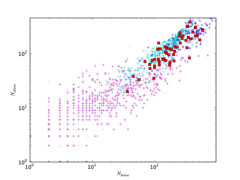
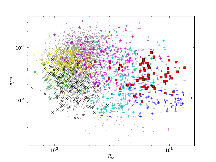
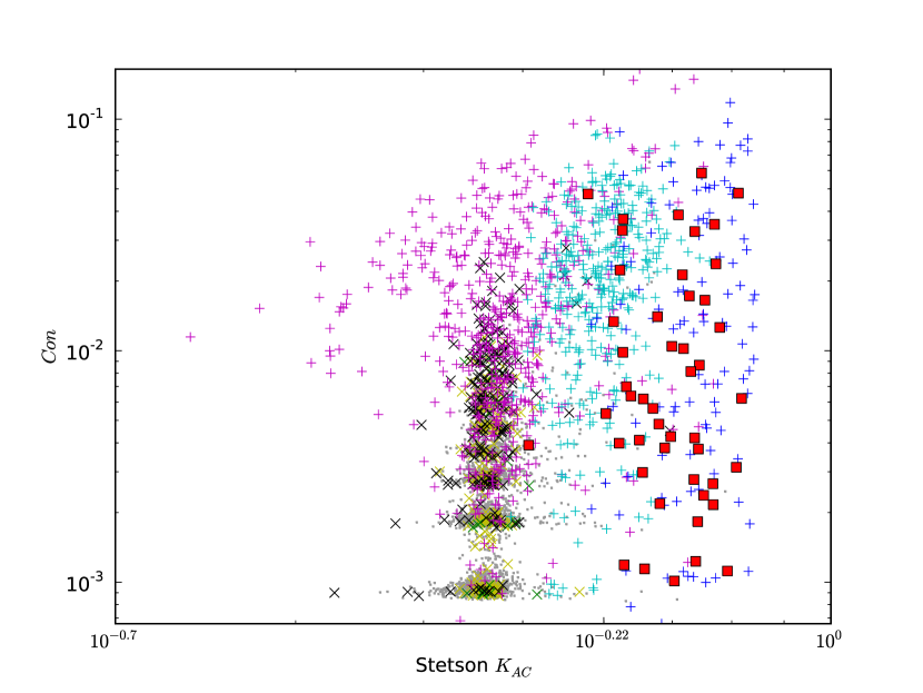
Figure 1.— Scatter plots of the 11 time series features. The axis of each panel is different time series feature. As the panels show, each type of variables is clustered in certain areas. 1) The top left panel: each type of the periodic variables are clustered at each different area. It also shows one day or multiple days period aliases caused by MACHO’s observational nightly pattern. 2) The top right panel: $\eta$ is relatively small for QSOs, Be stars and LPVs which have positive autocorrelation. Color (i.e. difference between average magnitude of MACHO $B$ and $R$ bands) is useful in separating QSOs from some other types of variables as several other studies suggested (Giveon et al., 1999; Eyer, 2002; Geha et al., 2003). 3) The middle left panel: $N_{above}$ vs $N_{below}$. The panel shows almost none of the non-variables and periodic variables except LPVs because they do not have data points above (below) the boundary lines by construction. 4) The middle right panel: $R_{cs}$ is relatively larger for QSOs. $\sigma/\bar{m}$ also separates some variable types. For instance, Be stars have relatively smaller values of $\sigma/\bar{m}$ than QSOs. 5) The bottom left panel: Stetson $L$ is effective in separating any type of variables from non-variables except microlensing events while Stetson $K_{AC}$ is practical to separate QSOs, Be stars and LPVs from others. 6) The bottom right panel: $Con$ can be used to separate non-variables from others because non-variables have relatively smaller $Con$ than the others. For details about each feature, see the text and Appendix.

Figure 1 shows scatter plots of all 11 time series features. Different colors and symbols denote different types of sources. The red squares are QSOs, the blue crosses are Be stars, the magenta crosses are microlensing events, the cyan crosses are LPVs, the green x’s are Cepheids, the yellow x’s are RR Lyraes, the black x’s are eclipsing binaries and the gray dots are non-variables. As each panel shows, not only QSOs but also other types of variables are clustered in certain areas, which means each time series feature is good at separating some of the variable types. Thus we did not implement a feature selection algorithm that removes uninformative features. See Section 4 for a brief explanation about a general feature selection concept. We selected a subset of MACHO lightcurves of each variable type to derive the time series features shown in the figure. We also used the same subset to train the classification model for selecting MACHO QSO candidates. For details about the training set, see Section 5.1.

A simple and conventional method for selecting QSOs using these features is to define cuts in the 2D-space shown in Figure 1 motivated by empirical observations of known classes. However, each panel exhibits a unique and complex structure of the features, which suggests that defining simple cuts is difficult. Moreover note that each panel in the figure is a 2D projection of the original 11D time series feature space. This implies that even if there exist proper cuts in the hyperspace that can separate the classes, these cuts could be obscured or invisible in any of the projections. Therefore, using simple cuts empirically derived from the projection could be inappropriate for the classification. In order to alleviate the problem of introducing empirical cuts and thus to fully utilize the derived 11 time series features, a classification algorithm should be capable of defining boundaries (e.g. cuts) in the hyperspace. For this purpose, we employed SVM which produces hyperplanes between classes in any multi-dimension space. SVM also can define non-linear boundaries using kernel functions while cuts are generally linear. In the following section, we briefly explain SVM.

4. Support Vector Machines

SVM (Boser et al., 1992) is a family of supervised machine learning algorithms that can train a 2-class classification model using samples of two known classes (i.e. training data). A SVM classifier can be seen as a single node neural network with an implicitly defined high dimensional feature space. It is currently one of the best classification methods in machine learning. Compared to neural networks SVM provide a flexible classification model, avoid the problems of local minima, and reduce the need for parameter tuning. Several efficient optimization methods have been developed for SVM training in recent years. For an overview, discussion and practical details the reader is referred to Cristianini & Shawe-Taylor (2000); Bennett & Campbell (2000); Hsu et al. (2003).

SVM have been applied extensively in many application areas, and in particular to various astronomical applications such as the classification of variable stars (Woźniak et al., 2004b), the selection of Active Galactic Nuclei (AGN) candidates (Zhang & Zhao, 2004), the determination of photometric redshift (Wadadekar, 2005), the classification of galaxies using synthetic galaxy spectra (Tsalmantza et al., 2007) and the morphological classification of galaxies using image data (Huertas-Company et al., 2008).

The classifier of a SVM defines a linear hyperplane that separates two classes in a training set. To select a unique hyperplane among the set of possible hyperplanes that separate the data, SVM chooses the hyperplane which maximizes the margin between the two classes, and is therefore often called the maximum margin separator. However, in many cases, it is not possible to find any hyperplane that can perfectly separate two classes. In other words, a training set of two classes cannot be separated without errors. In order to solve this problem, soft margin SVM which allows errors in a training set (i.e. mislabeled samples) was proposed (Cortes & Vapnik, 1995). The soft margin SVM uses a modified optimization criterion where a constant, $C>0$, controls a tradeoff between maximizing the margin and minimizing the errors of a classification model. The parameter $C$ needs to be selected appropriately in every application to balance the margin with the errors. Small $C$ allows a large margin between two classes and thus tends to ignore mislabeled samples. On the other hand, large $C$ allows a small margin and tries to separate even mislabeled samples. Another approach to address non-separability is to map the examples into a (typically high dimensional) feature space where the data might be better separated. Such mappings are captured implicitly by SVM as well as several other learning methods. To achieve this, SVM employ non-linear kernel functions that capture inner products in the implicit feature space. Intuitively the kernel can also be seen to be a similarity function acting in the expanded space. When this is done the hypothesis of SVM has the form:

$$Class(z)=\mbox{sign}(\sum_{i}\alpha_{i}y_{i}K(z,x_{i}))$$ (1)

where $z$ is the example we are predicting the label for, $x_{i}$ are the training data (i.e. the vectors of time series features), $y_{i}$ are the labels for the $i_{th}$ training data, and $i$ are indices for training examples. The $\alpha_{i}$ are the parameters learned by the training procedure. The construction of SVM shows that this form captures a linear separator in the feature space for which $K(z,x_{i})$ is an inner product, and the training procedure chooses the $\alpha_{i}$ that maximize the criterion of soft margin. Despite the mapping to a potentially high dimensional space, the maximum margin criterion leads to automatic capacity control and thus avoids overfitting.

Many forms of kernels exist in the literature, and the the most commonly used are the polynomial and the RBF (radial basis function) kernels. In this work, we followed standard practice (Hsu et al., 2003) and used the RBF defined as:

$$K(x_{i},x_{j})=\rm{exp}(-\gamma||x_{i}-x_{j}||^{2}),\,\,\gamma>0,$$ (2)

where $x_{i}$, $x_{j}$ are two examples, and the kernel parameter $\gamma$ determines the width of the kernel function. The implicit feature space in this case is known to be of infinite dimension. As in the case of the parameter $C$, the value of $\gamma$ needs to be selected appropriately for the application. One can readily observe that this kernel measures similarity between examples and that $\gamma$ controls how fast the similarity decays with respect to the distance between the examples. Seen in this light, the classifier (Equation 1) can also be seen to be a weighted form of nearest neighbor classification where the $\alpha_{i}$ weight the importance of training examples.

It is well known that the choice of $\gamma$ and $C$ can affect the results dramatically. In order to determine the best values for our application we used grid search with the 10-fold cross-validation and technique (Hsu et al., 2003).

• Cross-validation

  We divide each class into 10 subsets (i.e. 10-fold cross-validation) and select nine subsets to train a classification model. We then apply the trained model to the remaining subset and count the number of true positives (i.e. number of QSOs that the model identifies as QSOs), the number of false positives (i.e. number of non-QSOs that the model identifies as QSOs) and the number of false negatives (i.e. number of QSOs that the model identifies as non-QSOs). We repeat this process ten times with all different combinations. Finally we sum the true positives, false positives and false negatives from each iteration, and calculate the recall and precision defined as:

  $$\begin{array}[]{l}\displaystyle{\rm{recall}}=\frac{N_{TP}}{N_{TP}+N_{FN}},\,\,{\rm{precision}}=\frac{N_{TP}}{N_{TP}+N_{FP}},\end{array}$$ (4)

  where $N_{TP}$ is the sum of the true positives, $N_{FP}$ is the sum of the false positives and $N_{FN}$ is the sum of the false negatives.

• Grid search

  To select the best $C$ and $\gamma$, we search in a log-scale evenly spaced 10x10 grid with values from $10^{-1}$ to $10^{4}$. We then perform a 10-fold cross-validation and select $C$ and $\gamma$ that gave the best recall and the best precision. We then define a finer 10x10 grid and repeat the 10-fold cross-validation test with the new set of parameters. We repeat this procedure until recall and precision are not improving any more.

Standard SVM does not provide probability output. Thus we employed Platt’s probability estimation (Platt, 1999) to derive class probabilities. The Platt posterior probability is calculated using a sigmoid function as:

$$Pr(y=1|x)=\frac{1}{1+e^{Af+B}}\,\,,$$ (5)

where $f$ is a decision function such that ${\rm{sgn}}(f(x))$ decides the class of sample $x$. $y$ is the label for sample $x$ (i.e. a value for the class) and takes the values of +1 or -1. As Platt notes, this amounts to assuming that $f$ corresponds to the log-odds of the positive label; this assumption is not fully justified but has been shown to work well in many applications. The parameters $A$ and $B$ are calculated by minimizing the negative log-likelihood of a training data:

$$\begin{array}[]{l}\displaystyle{\rm{min}}\{-\sum_{i=1}^{l}(t_{i}\,{\rm{log}}(p_{i})+(1-t_{i})\,{\rm{log}}(1-p_{i}))\},\\ \\ \displaystyle t_{i}=\frac{y_{i}+1}{2},\,\,\,\displaystyle p_{i}=\frac{1}{1+e^{Af_{i}+B}},\end{array}$$ (9)

where $i$ are indices of training data, $l$ is the total number of the training data and $y_{i}$ is a label for $i_{th}$ example. The derived Platt class probabilities can be used to check the confidences of the predicted classes.

Many authors have studied feature selection methods to remove irrelevant features (e.g. see Blum & Langley 1997; Bradley & Mangasarian 1998; Weston et al. 2001; Li et al. 2003; Chen & Lin 2006 and references therein). Such feature selections could be useful when there are too many features (e.g. more than a few hundred) including both relevant and irrelevant features. However, Nilsson et al. (2006) found that most known feature selection methods occasionally discard even relevant features. This work also noticed that SVM is robust against uninformative features as long as there are a sufficient number of informative features. Another reason for feature selection is to reduce CPU time for extracting features and for training models when there exist a great number of features. Note that we employed only 11 time series features (see the previous section and Appendix), and all of them are informative for separating some of the classes as shown in Figure 1. Thus it is not necessary to implement feature selection methods in this work.

5. MACHO QSO Candidate Selections Using SVM Classification Models

5.1. Training Classification Models

Using the 11 time series features and SVM, we trained a classification model for selecting MACHO QSO candidates. To train the model, we first selected a training set which consists of 58 MACHO QSOs, 1,629 variable sources of known types (128 Be stars, 582 microlensing events, 193 eclipsing binaries, 288 RR Lyraes, 73 Cepheids and 365 LPVs) and 4,288 non-variable sources. We selected these variables from the list of known MACHO variable sources. Table 2 shows the number of the known MACHO variables we collected from SIMBAD’s MACHO variable catalog (Alcock et al., 2001) and also from several literature sources (Alcock et al., 1997c, a, b; Wood, 2000; Keller et al., 2002; Thomas et al., 2005). To select non-variable stars, we randomly chose a subset of MACHO lightcurves from a few MACHO LMC fields and removed all the known MACHO variables from the subset.

We then derived the 11 time series features for individual MACHO lightcurves in the training set. Before deriving the features, we removed all data points in each lightcurve with photometric errors greater than three times the average photometric errors. The photometric errors are given by the MACHO photometric pipeline (Alcock et al., 1999).

Table 2Number of known MACHO variables

Variable types	#	References
RR Lyraes	9,722	Alcock et al. (2001)
Cepheids	1,868	Alcock et al. (2001)
Eclipsing binaries	6,835	Alcock et al. (2001)
LPVs	3,049	Wood (2000)
Blue variables	1,262	Keller et al. (2002)
Microlensings	626	Alcock et al. (1997c, a, b)
		Thomas et al. (2005)
Be stars	136	private communication
		with Geha, M.
RR Lyraes	8,292	from a separate work done
Cepheids	1,452	by our group.
		see the text for details.${}^{\ref{footnote:gabe}}$
Total	33,242

We then employed a 2-class classification SVM using the RBF. We empirically found that 2-class SVM with the RBF achieves better recall and precision than 2- or multiple-class SVM with other kernels including linear kernel. We applied a 10-fold cross-validation and grid search to all the combinations of 2- or multiple-class SVM and different kernels. We found that 2-class SVM with the RBF showed the best recall and precision. To use a 2-class SVM, we defined the MACHO QSOs as the members of one class and all others as members of the other class. In order to derive the best $C$ and $\gamma$, we performed a 10-fold cross-validation and grid search using the training set as described in the previous section. We performed the test on each MACHO band; one for the B band and one for the R band. Table 3 shows the derived best recall and precision of each band. As can be seen from the table, the B (R) model shows 82.8 (72.4)% recall and 75% precision, which means the B (R) model misses 17.2 (27.6)% of the MACHO QSOs and has 25 (25)% false positive rate. For the B model, the false positives consist of 12 Be stars, three microlensing events and one LPV; for the R model, 11 Be stars and three microlensing events. Although the majority of the false positives were Be stars as expected, the models excluded more than 90% of the 128 Be stars in the training set. It is worth mentioning that recall and precision could vary depending on which set of variables and non-variables we choose to use as a training set. For instance, if we exclude the 128 Be stars from the training set, we can increase recall to 95% with a 7% false positive rate. We can further increase recall and precision if we also remove microlensing events and LPVs from the training set. However, note also that the higher recall and precision does not guarantee a better model because the model would not be able to distinguish QSOs from the false positives such as Be stars, microlensing events and LPVs when applied to the whole dataset.

Finally, we trained two models, one each for the MACHO B and R bands, using the derived best $C$, $\gamma$ on the whole training set. We used the trained models to select QSO candidates from the MACHO database (see Section 5.2). Although the rate of derived false positives mentioned in the previous paragraph is 25%, it should not be expected that the selected MACHO QSO candidates using the models would have 25% false positives. This is because the training set is not complete; also, it is nearly impossible to take into account every known type of variability existing in the MACHO database, which includes not only astronomical variables but also non-astronomical photometric defects or systematic errors. In addition, the fraction of QSO in the whole dataset is likely to be different than the training set. Thus the true false positive rate for the MACHO QSO candidates could be higher than 25%. We will come back to this point when we discuss crossmatching the candidate list with known catalogs in Section 6.

In addition, Figure 2 shows the Platt probabilities of the known MACHO QSOs for B (the top panel) and R (the bottom panel) band lightcurves. As the figure shows, the majority of the QSOs have higher probabilities than 80%. We used the Platt probability of each MACHO lightcurve to select MACHO QSO candidates (see Section 5.2).

Table 3Recall and precision during the cross-validation

Band	Recall	Precision	False Positives
B	82.8%	75.0%	25.0%
R	72.4%	75.0%	25.0%

Figure 2.— Platt probabilities for the known MACHO QSOs. The top (bottom) panel is the Platt probabilities of the B (R) band lightcurves.

5.2. MACHO QSO Candidate Selections

To select the MACHO QSO candidates, we first derived the 11 time series features for the whole 40 million MACHO LMC lightcurves. We removed the data points in each lightcurve which have photometric errors greater than three times the average photometric errors as we did during model training (see Section 5.1). We then applied the trained models to each lightcurve and derived the QSO Platt probability estimation. Finally we selected only the lightcurves which had the probability product of B and R bands higher than 25% (e.g. 50% probabilities in both B and R bands). Using the 25% cut, we selected 1,620 QSO candidates from the entire MACHO LMC database. We show example lightcurves of the QSO candidates in Figure 3. As the figure shows, all the lightcurves have strong and non-periodic flux variation, which is the variability characteristic of QSOs.

Figure 4 shows recall and false positive rates corresponding to the probability product cuts on the training set. Using the 25% cut, we correctly identified 82.8% of the known MACHO QSOs (48 out of 58) with a 0% false positive rate. Although a probability cut lower than 25% yields better recall and also a 0% false positive rate, we choose the 25% cut because our training set is not complete, as mentioned in the previous section.

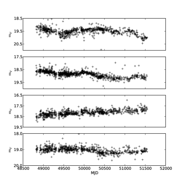
Figure 3.— Example lightcurves of the QSO candidates. The x-axis is modified Julian Date (MJD), and the y-axis is V magnitude, $m_{V}$. Each lightcurve manifests non-periodic and strong flux variation.

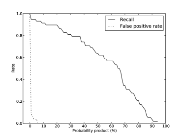
Figure 4.— Recall and false positive rate of the models based on the training set. Using 25% cut, we ca identify more than 80% of the known MACHO QSOs while removing all other variables and non-variables.

6. Crossmatching Results with Infrared and X-ray Catalogs

In order to estimate the true false positive rate without spectroscopic confirmation, we crossmatched the candidates with other astronomical catalogs. In the following subsections, we present the crossmatching results and the false positive rate estimated on the basis of the crossmatched counterparts.

6.1. Crossmatching with the Spitzer SAGE LMC catalog

It is known that mid-IR color selection is efficient at separating AGNs from other galaxies or stars because the spectral energy distributions of these types are substantially different from each other (Laurent et al., 2000; Lacy et al., 2004; Trichas et al., 2010; Kalfountzou et al., 2010). Based on these characteristics, Lacy et al. (2004) and Stern et al. (2005) introduced a mid-IR color cut to separate AGNs using the the Spitzer SAGE (Surveying the Agents of a Galaxy’s Evolution; Meixner et al. 2006) catalog. Kozłowski & Kochanek (2009) (hereinafter KK09) employed the mid-IR color cut and selected about 5,000 AGN candidates from the Spitzer SAGE catalog. KK09 also confirmed that the mid-IR color cut successfully identified most of the known QSOs in the SAGE footprints.

To check whether our candidates are inside the mid-IR selection cut that KK09 used, we crossmatched them with the Spitzer SAGE LMC catalog containing 6 million mid-IR objects and found 1,239 counterparts. We first searched the nearest SAGE source from each of the candidates within a 1^′′ search radius. In order to minimize false crossmatchings, we defined the source as a counterpart only if there exist no other Spitzer sources within a 3^′′ radius from the candidate.

Of the crossmatched counterparts, about 500 had been observed with at least three Spitzer IRAC (InfraRed Array Camera) bands. Note that we need a minimum of three Spitzer IRAC magnitudes to apply the mid-IR color cut. Figure 5 shows the color-color and color-magnitude diagrams of these counterparts (529 in the color-color diagram and 544 in the color-magnitude diagram). The solid line in the figure shows the mid-IR color selection cut. KK09 suggested that the sources inside region B could either be AGNs or black bodies such as stars, while the sources inside region A are likely AGNs (left panel). In the color-magnitude diagram (right panel), there are two regions as well. The region labeled as YSO is thought to be dominated by young stellar objects (YSO) while the region labeled QSO is thought to be dominated by QSOs. Nevertheless, all the sources inside these four regions (AGN region) are potential QSOs. According to Stern et al. (2005), the candidates inside the AGN region are most likely broad emission line QSOs (i.e. Type 1 AGNs). Among them, the sources inside the QSO and A regions are the most promising QSO candidates. As the figure clearly shows, most of the crossmatched QSO candidates are inside the QSO (88.2%; 480 out of 544) and the A regions (76.9%; 407 out of 529), which implies that most of the candidates are likely true QSOs. The number of QSO candidates that are in both the QSO and the A regions are 391 out of 529 (73.9%). Under the assumption that all the 391 candidates are QSOs, the false positive rate is 26.1%, which is the upper bound of the false positive rate. There are only about 9% of the candidates outside the AGN region (9.3% outside A and B regions, 9.0% outside YSO and QSO regions), giving us the lower bound of the false positive rate. Nevertheless, we confirmed that most of the candidates outside the AGN region also show strong variability. We show example lightcurves of these candidates in Figure 6. As the figure shows, they have strong and non-periodic flux variation. Note that our method used variability characteristics of lightcurves in order to select QSO candidates which could be missed by the mid-IR color selection. Moreover, the mid-IR color cut is not very efficient at selecting narrow emission line QSOs (Stern et al., 2005). Therefore some of the candidates could be either broad or narrow emission line QSOs even though they are not inside the AGN region, which would further decrease the lower bound of the false positive rate.

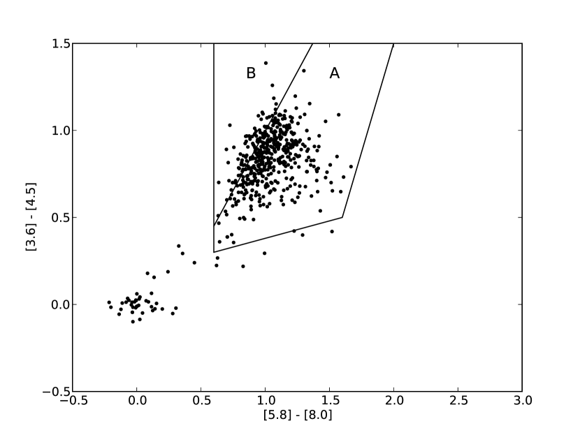
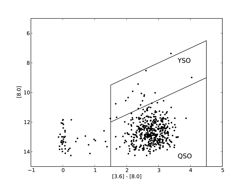
Figure 5.— Mid-IR color-color and color-magnitude diagrams of the Spitzer SAGE counterparts crossmatched with the QSO candidates. Each axis of the figure is either Spitzer magnitude or color. All sources inside the region A, B, QSO and YSO are potential QSOs (Kozłowski & Kochanek, 2009). The majority of the candidates are inside the region A and QSO, which is the most promising QSO regions.

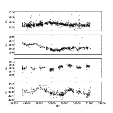
Figure 6.— Examples lightcurves of the QSO candidates outside the AGN region. The x-axis is MJD, and the y-axis is V magnitude. All of them show strong and non-periodic flux variation. These QSO candidates could either broad or narrow emission line QSOs although they are outside the AGN region.

In addition, we also crossmatched the known MACHO QSOs and the 33,242 MACHO variables shown in Table 2 with the SAGE catalog to check how many known MACHO QSOs and known variables are inside the AGN region. Such variables inside the AGN region could be contaminants (i.e. false positives) for any mid-IR color selection method. We found about 50 counterparts with the known MACHO QSOs and about 3,900 counterparts with the variables. We also crossmatched about 200,000 MACHO field sources from one randomly selected MACHO field with the SAGE catalog and found $\sim$10,000 counterparts. These field source counterparts might consist of all types of objects including non-variable stars, unclassified variable stars and galaxies. Figure 7 shows all the crossmatched counterparts. The black squares are the MACHO QSO counterparts (48 in the color-color diagram and 49 in the color-magnitude diagram). The black crosses are the counterparts with the variables including RR Lyraes, Cepheids, eclipsing binaries, LPVs and blue variable stars (3,871 in the color-color diagram and 3,880 in the color-magnitude diagram). We separately depict eight Be stars as gray diamonds in the figure. The gray dots are the MACHO field source counterparts (10,238 in the color-color diagram and 10,292 in the color-magnitude diagram). As the figure shows, almost all of the MACHO QSOs are inside the AGN region as expected. However, a few tens of the variables and the MACHO field sources are also inside the AGN region. We checked these variables in the AGN region and found that they consist of all types of the known MACHO variable stars such as RR Lyraes, Cepheids, eclipsing binaries, blue variables and LPVs. Moreover nearly all Be stars that have Spitzer counterparts are inside the region as well. It is known that Be stars are characterized by their IR emission due to dusty circumstellar environments (Malfait et al., 1998; Leinert et al., 2004). Also note that we crossmatched only 200,000 MACHO field sources with the Spitzer catalog. If we scaled our selection to the total MACHO LMC database covering 20 million stars, more than several thousand field sources would be in the AGN region, providing significant contaminantion for QSO selection. According to the results, it seems that the mid-IR cut is not efficient for separating QSO candidates from various types of stars although it is practical for confirming QSO candidates, especially when applied to massive databases. In other words, the mid-IR selection cut shows relatively low precision, although it shows high recall. Thus it is clear that algorithms based on the variability of lightcurves, including ours, are important for QSO candidate selections.

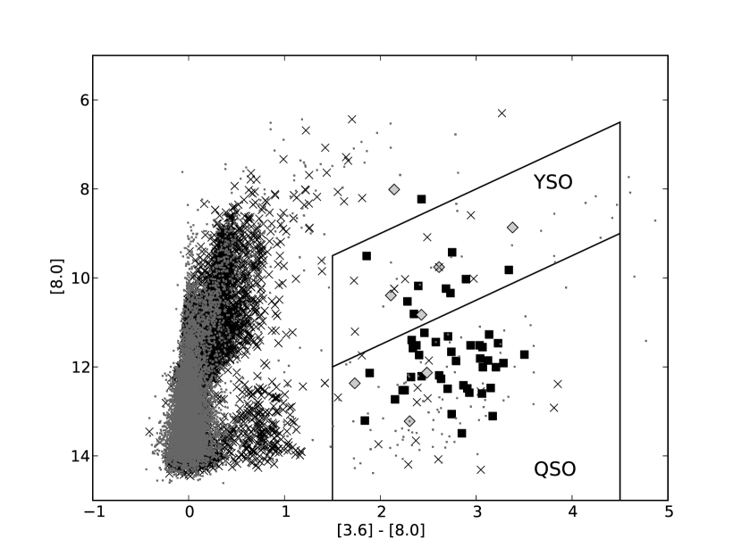
Figure 7.— Mid-IR colors of the Spitzer SAGE counterparts with the known MACHO variable stars and the MACHO field sources. Each axis of the figure is either Spitzer magnitude or color. The black squares are MACHO QSOs, the gray diamonds are Be stars, the black crosses are variable stars including RR Ryraes, Cepheids, eclipsing binaries, LPVs and blue variable stars. The gray dots are MACHO field sources. Almost all MACHO QSOs are inside the region A, B, QSO and YSO, which indicates the mid-IR selection criteria is efficient at confirming QSOs. However there are a lot of other variable stars including Be stars inside the regions as well. Thus the mid-IR selection might not be practical for selecting QSO candidates.

6.2. Crossmatching with X-ray Catalogs

We crossmatched our QSO candidates with the Chandra X-ray source catalog (Evans et al., 2009) and XMM-Newton 2^nd Incremental Source catalog (Watson et al., 2009). We searched for the nearest Chandra (XMM) source within a 5^′′ search radius from the candidate. We only selected the source as a counterpart if there existed no other Chandra (XMM) sources within the search radius. Nevertheless, most of the X-ray counterparts were placed within a 3^′′ distance from the candidates.

As a result, we found 60 X-ray counterparts. It is known that QSOs show higher X-ray to optical flux ratios than typical galaxies or stars, $f_{X}/f_{r}$, owing to the accretion on the central black holes (Reeves & Turner, 2000; Hornschemeier et al., 2001). To calculate $f_{X}/f_{r}$, we first derived the $m_{V}$ and $m_{R}$ (i.e. standard Johnson’s $V$ and Kron$-$Cousins $R$) using the MACHO B and R magnitudes (Alcock et al., 1999; Kunder & Chaboyer, 2008). We then converted the $m_{V}$ and $m_{R}$ to SDSS $r$ magnitude using the formula from the SDSS website (Lupton et al., 2005). Note that this formula was derived not based not on QSOs but on photometric standard stars (Stetson, 2000). Thus the converted SDSS $r$ magnitudes of QSOs could have larger errors (i.e. standard deviation) than the estimated errors for the standard stars, $\sigma\simeq 0.01$. Nevertheless, we finally used the following equation from Green et al. (2004) to derive ${\rm{log}}(f_{X}/f_{r})$:

$$\displaystyle{\rm{log}}\frac{f_{X}}{f_{r}}={\rm{log}}\,f_{X}+0.4\,r+5.67,$$ (10)

where $f_{X}$ is the X-ray flux in units of ergs cm^-2 s^-1 in the range of 0.5-2.0 keV, which is extracted from the Chandra and XMM catalogs. $f_{r}$ is the optical flux and $r$ is the converted SDSS $r$ magnitude.

The top panel of Figure 8 shows the $f_{X}/f_{r}$ of 60 counterparts with the Chandra and XMM catalogs. The x-axis is ${\rm{log}}(f_{X}/f_{r})$, and the y-axis is the converted $r$ magnitude. In the panel, we also show 16 known MACHO QSOs that have X-ray counterparts. The black marks are the MACHO QSO counterparts, and the gray marks are the QSO candidate counterparts. The squares are XMM counterparts, and the triangles are Chandra counterparts. The dashed line corresponds to $f_{X}/f_{r}=0.1$, which is the criterion separating AGNs and typical galaxies or stars (Green et al., 2004). The two dash-dotted lines are boundaries of the confusion area shown as the dashed area in the bottom panel (see the following paragraph). As the figure shows, most of the MACHO QSOs (75.0%; 12 out of 16) and our QSO candidates (73.3%; 44 out of 60) show higher $f_{X}/f_{r}$ than 0.1. If all the candidates with higher $f_{X}/f_{r}$ than 0.1 are QSOs, the false positive rate is 27.3%.

In addition, to estimate how a large portion of non-AGNs could have $f_{X}/f_{r}\geq 0.1$, we crossmatched all the objects from one MACHO field with the Chandra X-ray catalog. We selected the field so that it overlapped with the Chandra footprints. In the top panel of Figure 8, we show the $f_{X}/f_{r}$ of the 21 crossmatched MACHO objects (black dots). These counterparts could be either stars or AGNs, although they are most likely X-ray emitting stars such as X-ray binaries, W-UMa binaries (Chen et al., 2006), Algol type binaries (Singh et al., 1995) and cataclysmic variable stars (e.g. see Wonnacott et al. 1994) since the number density of such stars surpasses the number density of AGNs. Of the 21 MACHO objects, 16) have $f_{X}/f_{r}$ smaller than 0.1, which implies that non-AGN objects generally have smaller $f_{X}/f_{r}$ than 0.1. The remaining five objects have $f_{X}/f_{r}$ larger than 0.1 and could be AGN candidates. We show the lightcurves of these five objects in Figure 9. As the figure shows, they do not manifest any strong flux variation and thus were not selected as QSO candidates by our selection method.

Based on the crossmatching results mentioned in the previous paragraphs, we further improved the region of confidence using the histogram of ${\rm{log}}(f_{X}/f_{r})$ shown in the bottom panel of Figure 8. The x-axis is ${\rm{log}}(f_{X}/f_{r})$, and the y-axis is normalized count. The solid line with light gray is the histogram of the QSO candidate counterparts, the dashed line with medium gray is the histogram of the MACHO QSO counterparts and the dotted line with dark gray is the histogram of the 21 MACHO object counterparts. The dashed area shows the confusion area where stars and QSOs could be mixed together. Considering all the histograms, we modified the confidence regions as:

• log$(f_{X}/f_{r})<-1.5$ : the non-QSO area

  In this region, log($f_{X}/f_{r}$) is much smaller than the AGN criterion of log$(f_{X}/f_{r})=-1$. Thus the candidates in this region are not likely QSOs. There are only 1 out of 16 (6.2%) MACHO QSOs, 4 out of 21 (19%) MACHO objects, 7 out of the 60 (11%) candidates inside this region.

• $-1.5\leq f_{X}/f_{r}<-0.5$ : the confusion area that is a mixture of stars and QSOs

  Most of the MACHO objects (76.2%; 16 out of 21) are in this region. More than a half of the MACHO QSOs (55.3%; 9 out of 16) and 32 out of the 60 QSO candidates (53.3%) are also in this region.

• $f_{X}/f_{r}\geq-0.5$ : the QSO area

  Most of the candidates in this region would be QSOs because of their high $f_{X}/f_{r}$. As the histogram shows, only 1 out of 21 (5%) MACHO objects is in this region while 6 out of 16 (37.5%) MACHO QSOs and 21 out of 60 (35%) candidates are inside the region.

As we mentioned above, 21 out of the 60 candidates are inside the QSO area and are likely true QSOs, which gives the upper bound of the false positive rate, 65.0% (39/60). In addition, some of the 32 candidates inside the confusion area could be also QSOs because more than half of the known MACHO QSOs are inside the confusion area. Thus the lower bound of the false positive rate is 11.7% (7/60).

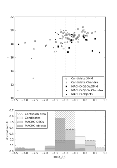
Figure 8.— $f_{X}/f_{r}$ of the X-ray counterparts with the MACHO QSOs, the QSO candidates and the MACHO field objects. The top panel: the x-axis is log($f_{X}/f_{r}$), and the y-axis is the converted SDSS $r$ magnitude. The squares are the XMM counterparts and the triangles are the Chandra counterparts. The black marks are the MACHO QSOs and the gray marks are the candidates. The gray dots are the MACHO field objects. The dashed line is the criterion between AGN and others such as galaxies and stars. Most of the MACHO QSOs and the candidates have higher $f_{X}/f_{r}$ than the criterion while most of the MACHO field objects have smaller $f_{X}/f_{r}$ than the criterion, which implies most of the candidates are promising QSO candidates. The bottom panel: the histogram of $f_{X}/f_{r}$. The x-axis is log($f_{X}/f_{r}$), and the y-axis is normalized count. Based on the histogram, we refined the region of confidence. See the text for details.

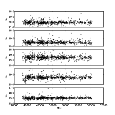
Figure 9.— Lightcurves of 5 MACHO field objects which have higher $f_{X}/f_{r}$ than the AGN criterion. The x-axis is MJD, and the y-axis is V magnitude, $m_{V}$. Although they have higher $f_{X}/f_{r}$ than the criterion, they do not have strong flux variation and thus were not selected as QSO candidates by our selection algorithm.

7. Ongoing and Future Works

We will observe the QSO candidates with spectroscopic instruments to check whether they are QSOs. Based on the projection of the models and the crossmatching results, we expect at least several hundred candidates to turn out to be QSOs.

Using the confirmed QSOs and the false positives, we will improve our model. The current model is constructed based on the relatively small number of known QSOs (i.e. 58 known MACHO QSOs), which may be too small a sample to represent the true variability characteristics of all QSOs in the MACHO database. Thus using a large number of QSOs (i.e. more than a few hundreds) would help improve the models.

In addition, our model is effective at selecting not only QSOs but also other types of variable sources. Preliminary tests showed that recall and precision for periodic variables such as RR Lyraes, Cepheids and eclipsing binaries, were almost 100%; for LPVs, microlensing events and Be stars, recall and precision were 80%.

8. Summary

In this paper, we presented a new QSO selection algorithm based on 11 time series features and a supervised classification. We first introduced 11 time series features to quantify variability characteristics of lightcurves. We then used Support Vector Machine (SVM) to train a classification model which separates QSOs from other types of variable stars and non-variable stars. Using the training set of the MACHO variables (128 Be stars, 582 microlensing events, 193 eclipsing binaries, 288 RR Lyraes, 73 Cepheids and 365 LPVs), 4,288 non-variables and the 58 known MACHO QSOs, we trained the models for each MACHO B and R band. The trained model correctly identified about 80% of the MACHO QSOs with 25% false positive rates on a cross-validation test. The majority of false positives during the training were Be stars known to show variability similar to with QSOs.

We applied the model to the whole MACHO LMC database consisting of 40 million lightcurves (i.e. 20 million from each MACHO band) in order to select QSO candidates. As a result, we found 1,620 candidates from the MACHO LMC database. During the selection, none of the known MACHO variables were mis-selected as QSO candidates. To estimate the true false positive rate of the QSO candidates, we crossmatched the candidates with astronomical catalogs, including the Spitzer SAGE LMC catalog and some X-ray catalogs. The crossmatching results confirmed that most of our candidates are promising QSO candidates. For instance, the majority of candidates with Spitzer counterparts are inside the AGN region that is defined by a mid-IR color cut and is known to be effective in confirming QSO candidates. The crossmatching with X-ray catalogs shows that most of the X-ray counterparts have $f_{X}/f_{r}\geq 0.1$ and therefore are likely QSOs.

In addition, during the crossmatching with the SAGE LMC catalog, we found that using only the mid-IR color cut is not a very efficient method in selecting QSO candidates, although it is an effective method in confirming QSOs. This suggests that selection methods using variability characteristics of lightcurves, including ours, are important to further remove false positives, both variables and non-variables.

Appendix

In this appendix, we introduce the 11 time series features including four new features that we have developed for this work and the remaining seven features.

Four new time series features:

• Three autocorrelation Indices

  These three indices are based on the autocorrelation function. The autocorrelation function is defined as:

  $$AC(\tau)=\displaystyle\frac{1}{(N-\tau)\,\,\sigma^{2}}\,\sum_{i=1}^{N-\tau}(m_{i}-\bar{m})(m_{i+\tau}-\bar{m}),$$ (11)

  where $N$ is the total number of data points, $\tau=1,2,\ldots,N-1$ is the time lag, $\sigma$ is the standard deviation, $m$ is the magnitude, $i$ is the index for each data point and $\bar{m}$ is the mean magnitude. Figure 10 shows the $AC(\tau)$ for various types of variables and non-variables extracted from the MACHO database. Note that, in each panel, we show the $AC(\tau)$ of multiple objects of that type to demonstrate the overall $AC(\tau)$ patterns. We used more than 50 objects of non-variables, RR lyraes, Cepheids, eclipsing binaries and microlensing events. The overall $AC(\tau)$ patterns were preserved even if we used more objects (i.e. several hundreds). For long period variables (LPVs), Be stars and QSOs, we used about 10 object of each type to show individual $AC(\tau)$ pattern. The x-axis is the time lag, $\tau$ in days and the y-axis is the autocorrelation value. As the figure shows, non-variables and all periodic variables but LPVs show different $AC(\tau)$ patterns from QSOs, Be stars, LPVs and microlensing events. Schild et al. (2009) also noticed that the $AC(\tau)$ could be useful for discovering QSOs. Thus, by quantifying the $AC(\tau)$, we can separate certain types of variables. In the following paragraphs, we introduce three time series features that we are using to quantify $AC(\tau)$.

  

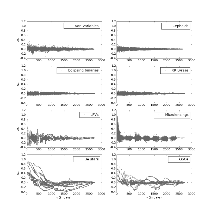
  Figure 10.— Set of autocorrelation functions of variable and non-variable stars. The x-axis is the time lag, $\tau$, in days, and the y-axis is the autocorrelation function value. Non-variable stars, Cepheids, eclipsing binaries and RR Lyraes show different patterns from QSOs, Be stars, LPVs and microlensing events.

  • $N_{above}$, $N_{below}$

    We constructed empirical boundary lines on the AC vs $\tau$ diagram to separate non-variables and periodic variables from others. To do so, we calculated the average and standard deviation of the autocorrelation functions for non-variables and periodic variables (except LPVs), for each time lag $\tau$. We then constructed upper and lower boundary lines to be $\pm 4\sigma$ from the average line. Figure 11 shows the calculated upper and lower boundary lines. To derive $N_{above}$ and $N_{below}$ for each lightcurve, we counted the number of points above, $N_{above}$, and number of points below, $N_{below}$, these lines.

  • Stetson $K$

    Stetson $K$ (Eq. 23) was defined to observe the distribution of measurements between the maximum and minimum values of the measurements (Stetson, 1996). For details including the definition of Stetson $K$, see the Appendix. We used Stetson $K$ to characterize the different $AC(\tau)$ patterns, Stetson $K_{AC}$.

• $R_{cs}$

  $R_{cs}$ is the range of a cumulative sum (Ellaway, 1978) of each lightcurve and is defined as:

  $$\begin{array}[]{l}R_{cs}={\rm{max}}(S)-{\rm{min}}(S),\\ \\ S_{l}=\displaystyle\frac{1}{N\,\,\sigma}\sum_{i=1}^{l}(m_{i}-\bar{m})\,,\end{array}$$ (15)

  where max (min) is the maximum (minimum) value of $S$ and $l=1,2,\ldots,N$. $R_{cs}$ is typically large for LPVs, microlensing events, Be stars and QSOs while it is relatively small for non-variables and other periodic variables such as RR Lyraes, Cepheids and eclipsing binaries.

  

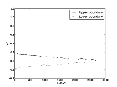
  Figure 11.— Two boundary lines constructed using autocorrelation functions of non-variable stars, eclipsing binaries, RR Lyraes and Cepheids. The x-axis is the time lag, $\tau$, in days, and the y-axis is the autocorrelation value. Based on the lines, we derived $N_{above}$ and $N_{below}$. See the text for details.

Other seven time series features:

• $\displaystyle\frac{\sigma}{\bar{m}}$

  This is a simple variability index and is defined as the ratio of the standard deviation, $\sigma$, to the mean magnitude, $\bar{m}$. If a lightcurve has strong variability, $\sigma/\bar{m}$ of the lightcurve is generally large.

• Period and Period S/N

  To derive periods and their signal to noise ratios (S/N), we employed the Lomb-Scargle algorithm (Lomb, 1976; Scargle, 1982; Press & Rybicki, 1989; Press et al., 1992). We search for periods between 0.1 and 1000 days, which covers not only short period variable stars such as RR Lyraes, Cepheids and eclipsing binaries but also LPVs. Among the detected periods, we selected the period with the highest S/N. The S/N of each period is calculated based on the Lomb periodogram (Scargle, 1982; Press et al., 1992).

• Stetson $L$

  Stetson $L$ variability index (Stetson, 1996) describes the synchronous variability of different bands and is defined as:

  $$L=\frac{JK}{0.798}\,,$$ (16)

  where $J$ and $K$ are different Stetson indices. Stetson $J$ is calculated based on two simultaneous lightcurves of a same star (e.g. MACHO B and R bands) and is defined as:

  $$\begin{array}[]{l}\displaystyle J=\frac{1}{N}\sum_{i=1}^{N}{\rm{sgn}}(P_{i})\sqrt{|P_{i}|},\\ \\ \displaystyle P_{i}=\delta_{p}(i)\,\delta_{q}(i),\\ \\ \displaystyle\delta_{p}(i)=\sqrt{\frac{N}{N-1}}\,\,\frac{m_{p,i}-\bar{m}}{\sigma_{p,i}},\end{array}$$ (22)

  where $i$ is the index for each data point, $N$ is the total number of data points, sgn($P_{i}$) is the sign of $P_{i}$ and $m$ is the magnitude. $p$ and $q$ indicate two different bands. $\sigma_{p,i}$ is the standard error of $i_{th}$ magnitude of band $p$. In case of the MACHO database, $p$ and $q$ indicate the MACHO B and R bands. To derive $J$ from each MACHO time series, we used only the data points which have observations from both MACHO B and R bands at the same epoch.

  Steston $K$ is calculated using a single band lightcurve and is defined as:

  $$K=\frac{1}{\sqrt{N}}\frac{\sum_{i=1}^{N}|\delta(i)|}{\sqrt{\sum_{i=1}^{N}\delta(i)^{2}}}.$$ (23)

  It is known that $K=0.900$ for a pure sinusoid and 0.798 for a Gaussian distribution. For details, see Stetson (1996).

  In brief, Stetson $L$ is generally large for achromatic variable sources and small for non-variables or chromatic variables.

• $\eta$

  Variability index $\eta$ is the ratio of the mean of the square of successive differences to the variance of data points. The index was originally proposed to check whether the successive data points are independent or not. In other words, the index was developed to check if any trends exist in the data (von Neumann, 1941). It is defined as:

  $$\eta=\frac{1}{(N-1)\,\,\sigma^{2}}\sum_{i=1}^{N-1}(m_{i+1}-m_{i})^{2}.$$ (24)

  The index has been substantially investigated by several authors (see von Neumann 1941; Press 1969 and references therein). In brief, if there exists positive serial correlation, $\eta$ is relatively small. On the other hand, if there exists negative serial correlation, $\eta$ is large. Shin et al. (2009) used $\eta$ to select variable candidates from the Northern Sky Variability Survey database (Woźniak et al., 2004a).

  As the top right panel of Figure 1 shows, $\eta$ is relatively small for the variables which have positive autocorrelation such as QSOs, Be stars and LPVs. Non-variables or microlensing events show large $\eta$ since they do not have strong positive correlation. In the cases of other periodic variables such as RR Lyraes, Cepheids and eclipsing binaries, $\eta$ is also relatively large even though they are periodic variables and therefore have positive correlation. This is because 1) we derive $\eta$ not from the folded MACHO lightcurves but from the original lightcurves and 2) MACHO observed a field a few times per week, which is not enough to reveal positive correlation for small time scales. In other words, most raw MACHO lightcurves of the periodic variables do not have strong positive correlation and thus have large $\eta$.

• $B-R$

  We used an average color for each MACHO lightcurve as:

  $$B-R=\displaystyle\bar{m}_{{B}_{M}}-\bar{m}_{{R}_{M}},$$ (25)

  where $\bar{m}_{{B}_{M}}$, $\bar{m}_{{R}_{M}}$ are the mean magnitudes of MACHO B, R bands.

  Color information, $B-R$, is useful in separating QSOs from some other types of variables as several other studies suggested (Giveon et al., 1999; Eyer, 2002; Geha et al., 2003). Nevertheless it is known that color is not very efficient discriminator for selecting intermediate redshift QSOs (i.e. $2.5<z<3.0$) although it is efficient for selecting high and low redshift QSOs (Richards et al., 2006; Schmidt et al., 2010). Note that we used not only color information but also other multiple time series features derived solely based on the variability characteristics of lightcurves, which helps to identify intermediate redshift QSOs as well as high and low redshift QSOs.

• $Con$

  The index was introduced for the selection of variable stars from the OGLE database (Woźniak, 2000). To calculate $Con$, we counted the number of three consecutive data points that are brighter or fainter than 2$\sigma$ and normalized the number by $N-2$. $Con$ is close to zero for non-variable stars while it is relatively large for variables. In addition, $Con$ is relatively large for the long-time scale varying sources such as LPVs because such variables tend to have plenty of consecutive data points bigger than 2$\sigma$.

References

- Alcock et al. (2001) Alcock, C., Allsman, R., Alves, D. R., & et al. 2001, Variable Stars in the Large Magellanic Clouds, VizieR Online Data Catalog (http://vizier.u-strasbg.fr/viz-bin/VizieR?-source=II/247)
- Alcock et al. (1997a) Alcock, C., Allsman, R. A., Alves, D. R., & et al. 1997a, ApJ, 491, L11+
- Alcock et al. (1997b) —. 1997b, ApJ, 479, 119
- Alcock et al. (1997c) —. 1997c, ApJ, 486, 697
- Alcock et al. (1999) —. 1999, PASP, 111, 1539
- Alcock et al. (2000) —. 2000, ApJ, 542, 281
- Alcock et al. (1996) Alcock, C., Allsman, R. A., Axelrod, T. S., & et al. 1996, ApJ, 461, 84
- Aretxaga et al. (1997) Aretxaga, I., Cid Fernandes, R., & Terlevich, R. J. 1997, MNRAS, 286, 271
- Bauer et al. (2009) Bauer, A., Baltay, C., Coppi, P., & et al. 2009, ApJ, 696, 1241
- Becker et al. (2001) Becker, R. H., Fan, X., White, R. L., & et al. 2001, AJ, 122, 2850
- Bennett & Campbell (2000) Bennett, K. P., & Campbell, C. 2000, SIGKDD Explorations, 2, 1
- Blanco & Heathcote (1986) Blanco, V. M., & Heathcote, S. 1986, PASP, 98, 635
- Blum & Langley (1997) Blum, A. L., & Langley, P. 1997, Artificial Intelligence, 97, 245 , relevance
- Boser et al. (1992) Boser, B. E., Guyon, I. M., & Vapnik, V. N. 1992, in Proceedings of the fifth annual workshop on Computational learning theory, COLT ’92 (New York, NY, USA: ACM), 144–152
- Bradley & Mangasarian (1998) Bradley, P. S., & Mangasarian, O. L. 1998, in ICML ’98: Proceedings of the Fifteenth International Conference on Machine Learning (San Francisco, CA, USA: Morgan Kaufmann Publishers Inc.), 82–90
- Butler & Bloom (2010) Butler, N. R., & Bloom, J. S. 2010, ArXiv e-prints
- Chang & Lin (2001) Chang, C. C., & Lin, C. J. 2001, LIBSVM : a library for support vector machines, http://www.csie.ntu.edu.tw/cjlin/libsvm
- Chen et al. (2006) Chen, W. P., Sanchawala, K., & Chiu, M. C. 2006, AJ, 131, 990
- Chen & Lin (2006) Chen, Y.-W., & Lin, C.-J. 2006, in Studies in Fuzziness and Soft Computing, Vol. 207, Feature Extraction, ed. I. Guyon, M. Nikravesh, S. Gunn, & L. Zadeh (Springer Berlin, Heidelberg), 315–324
- Cortes & Vapnik (1995) Cortes, C., & Vapnik, V. 1995, Machine Learning, 20, 273
- Cristiani et al. (1996) Cristiani, S., Trentini, S., La Franca, F., & et al. 1996, A&A, 306, 395
- Cristianini & Shawe-Taylor (2000) Cristianini, N., & Shawe-Taylor, J. 2000, An Introduction to Support Vector Machines (Cambridge: Cambridge Univ. Press)
- de Vries et al. (2005) de Vries, W. H., Becker, R. H., White, R. L., & et al. 2005, AJ, 129, 615
- Dobrzycki et al. (2005) Dobrzycki, A., Eyer, L., Stanek, K. Z., & et al. 2005, A&A, 442, 495
- Dobrzycki et al. (2002) Dobrzycki, A., Groot, P. J., Macri, L. M., & et al. 2002, ApJ, 569, L15
- Ellaway (1978) Ellaway, P. 1978, Electroencephalography and Clinical Neurophysiology, 45, 302
- Evans et al. (2009) Evans, I., Primini, F. A., Glotfelty, K. J., & et al. 2009, in Chandra’s First Decade of Discovery, Proceedings of the conference held 22-25 September, 2009 in Boston, MA. Edited by Scott Wolk, Antonella Fruscione, and Douglas Swartz, abstract #94, ed. S. Wolk, A. Fruscione, & D. Swartz
- Eyer (2002) Eyer, L. 2002, Acta Astronomica, 52, 241
- Fan et al. (2006) Fan, X., Strauss, M. A., Becker, R. H., & et al. 2006, AJ, 132, 117
- Geha et al. (2003) Geha, M., Alcock, C., Allsman, R. A., & et al. 2003, AJ, 125, 1
- Giveon et al. (1999) Giveon, U., Maoz, D., Kaspi, S., & et al. 1999, MNRAS, 306, 637
- Green et al. (2004) Green, P. J., Silverman, J. D., Cameron, R. A., & et al. 2004, ApJS, 150, 43
- Hartman et al. (2008) Hartman, J. D., Gaudi, B. S., Holman, M. J., & et al. 2008, ApJ, 675, 1254
- Hawkins (1993) Hawkins, M. R. S. 1993, Nature, 366, 242
- Hawkins (2002) —. 2002, MNRAS, 329, 76
- Hook et al. (1994) Hook, I. M., McMahon, R. G., Boyle, B. J., & et al. 1994, MNRAS, 268, 305
- Hornschemeier et al. (2001) Hornschemeier, A. E., Brandt, W. N., Garmire, G. P., & et al. 2001, ApJ, 554, 742
- Hsu et al. (2003) Hsu, C.-W., Chang, C.-C., & Lin, C.-J. 2003, A practical guide to support vector classification, Tech. rep., Department of Computer Science, National Taiwan University
- Huertas-Company et al. (2008) Huertas-Company, M., Rouan, D., Tasca, L., & et al. 2008, A&A, 478, 971
- Ivezic et al. (2008) Ivezic, Z., Tyson, J. A., Allsman, R., Andrew, J., Angel, R., & for the LSST Collaboration. 2008, ArXiv e-prints
- Kaiser (2004) Kaiser, N. 2004, in Society of Photo-Optical Instrumentation Engineers (SPIE) Conference Series, Vol. 5489, Society of Photo-Optical Instrumentation Engineers (SPIE) Conference Series, ed. J. M. Oschmann Jr., 11–22
- Kalfountzou et al. (2010) Kalfountzou, E., Trichas, M., Rowan-Robinson, M., & et al. 2010, ArXiv e-prints
- Kawaguchi et al. (1998) Kawaguchi, T., Mineshige, S., Umemura, M., & et al. 1998, ApJ, 504, 671
- Keller et al. (2002) Keller, S. C., Bessell, M. S., Cook, K. H., & et al. 2002, AJ, 124, 2039
- Kelly et al. (2009) Kelly, B. C., Bechtold, J., & Siemiginowska, A. 2009, ApJ, 698, 895
- Kollmeier et al. (2006) Kollmeier, J. A., Onken, C. A., Kochanek, C. S., & et al. 2006, ApJ, 648, 128
- Kozłowski & Kochanek (2009) Kozłowski, S., & Kochanek, C. S. 2009, ApJ, 701, 508
- Kozłowski et al. (2010) Kozłowski, S., Kochanek, C. S., Udalski, A., & et al. 2010, ApJ, 708, 927
- Kunder & Chaboyer (2008) Kunder, A., & Chaboyer, B. 2008, AJ, 136, 2441
- Lacy et al. (2004) Lacy, M., Storrie-Lombardi, L. J., Sajina, A., & et al. 2004, ApJS, 154, 166
- Laurent et al. (2000) Laurent, O., Mirabel, I. F., Charmandaris, V., Gallais, P., Madden, S. C., Sauvage, M., Vigroux, L., & Cesarsky, C. 2000, A&A, 359, 887
- Leinert et al. (2004) Leinert, C., van Boekel, R., Waters, L. B. F. M., & et al. 2004, A&A, 423, 537
- Li et al. (2003) Li, C., Liu, F., & Xie, Y. 2003, Computational Intelligence and Multimedia Applications, International Conference on, 0, 37
- Lomb (1976) Lomb, N. R. 1976, Ap&SS, 39, 447
- Lupton et al. (2005) Lupton, R. H., Jurić, M., Ivezić, Z., & et al. 2005, in Bulletin of the American Astronomical Society, Vol. 37, Bulletin of the American Astronomical Society, 1384–+
- MacLeod et al. (2010) MacLeod, C. L., Brooks, K., Ivezic, Z., & et al. 2010, ArXiv e-prints
- Malfait et al. (1998) Malfait, K., Bogaert, E., & Waelkens, C. 1998, A&A, 331, 211
- Meixner et al. (2006) Meixner, M., Gordon, K. D., Indebetouw, R., & et al. 2006, AJ, 132, 2268
- Mennickent et al. (2002) Mennickent, R. E., Pietrzyński, G., Gieren, W., & et al. 2002, A&A, 393, 887
- Metcalf & Madau (2001) Metcalf, R. B., & Madau, P. 2001, ApJ, 563, 9
- Miranda & Macciò (2007) Miranda, M., & Macciò, A. V. 2007, MNRAS, 382, 1225
- Nilsson et al. (2006) Nilsson, R., J., P., Björkegren, J., & et al. 2006, Lecture Notes in Computer Science, Vol. 4212, Evaluating Feature Selection for SVMs in High Dimensions, ed. J. Fürnkranz, T. Scheffer, & M. Spiliopoulou (Springer Berlin, Heidelberg), 719–726
- Panik (2005) Panik, M. J. 2005, Advanced statistics from an elementary point of view (San Diego, CA: Elsevier Academic Press), 576
- Peng et al. (2006) Peng, C. Y., Impey, C. D., Rix, H., & et al. 2006, ApJ, 649, 616
- Platt (1999) Platt, J. C. 1999, in Advances in Large Margin Classifiers (MIT Press), 61–74
- Press (1969) Press, S. J. 1969, The Annals of Mathematical Statistics, 40, 188
- Press & Rybicki (1989) Press, W. H., & Rybicki, G. B. 1989, ApJ, 338, 277
- Press et al. (1992) Press, W. H., Teukolsky, S. A., Vetterling, W. T., & et al. 1992, Numerical recipes in C. The art of scientific computing, ed. Press, W. H., Teukolsky, S. A., Vetterling, W. T., & Flannery, B. P.
- Rees (1984) Rees, M. J. 1984, ARA&A, 22, 471
- Reeves & Turner (2000) Reeves, J. N., & Turner, M. J. L. 2000, MNRAS, 316, 234
- Richards et al. (2006) Richards, G. T., Strauss, M. A., Fan, X., & et al. 2006, AJ, 131, 2766
- Ross et al. (2009) Ross, N. P., Shen, Y., Strauss, M. A., & et al. 2009, ApJ, 697, 1634
- Scargle (1982) Scargle, J. D. 1982, ApJ, 263, 835
- Schild et al. (2009) Schild, R. E., Lovegrove, J., & Protopapas, P. 2009, AJ, 138, 421
- Schmidt et al. (2010) Schmidt, K. B., Marshall, P. J., Rix, H., & et al. 2010, ApJ, 714, 1194
- Schmidtke et al. (1999) Schmidtke, P. C., Cowley, A. P., Crane, J. D., & et al. 1999, AJ, 117, 927
- Sesar et al. (2007) Sesar, B., Ivezić, Ž., Lupton, R. H., & et al. 2007, AJ, 134, 2236
- Shen et al. (2007) Shen, Y., Strauss, M. A., Oguri, M., & et al. 2007, AJ, 133, 2222
- Shin et al. (2009) Shin, M., Sekora, M., & Byun, Y. 2009, MNRAS, 400, 1897
- Simcoe et al. (2004) Simcoe, R. A., Sargent, W. L. W., & Rauch, M. 2004, ApJ, 606, 92
- Singh et al. (1995) Singh, K. P., Drake, S. A., & White, N. E. 1995, ApJ, 445, 840
- Stern et al. (2005) Stern, D., Eisenhardt, P., Gorjian, V., & et al. 2005, ApJ, 631, 163
- Stetson (1996) Stetson, P. B. 1996, PASP, 108, 851
- Stetson (2000) —. 2000, PASP, 112, 925
- Sumi et al. (2005) Sumi, T., Woźniak, P. R., Eyer, L., & et al. 2005, MNRAS, 356, 331
- Terlevich et al. (1992) Terlevich, R., Tenorio-Tagle, G., Franco, J., & et al. 1992, MNRAS, 255, 713
- Thomas et al. (2005) Thomas, C. L., Griest, K., Popowski, P., & et al. 2005, ApJ, 631, 906
- Trichas et al. (2010) Trichas, M., Rowan-Robinson, M., Georgakakis, A., & et al. 2010, MNRAS, 405, 2243
- Tsalmantza et al. (2007) Tsalmantza, P., Kontizas, M., Bailer-Jones, C. A. L., & et al. 2007, A&A, 470, 761
- Udalski et al. (1997) Udalski, A., Kubiak, M., & Szymanski, M. 1997, Acta Astronomica, 47, 319
- Udalski et al. (2008) Udalski, A., Szymanski, M. K., Soszynski, I., & et al. 2008, Acta Astronomica, 58, 69
- Vanden Berk et al. (2004) Vanden Berk, D. E., Wilhite, B. C., Kron, R. G., & et al. 2004, ApJ, 601, 692
- Viel et al. (2002) Viel, M., Matarrese, S., Mo, H. J., & et al. 2002, MNRAS, 329, 848
- von Neumann (1941) von Neumann, J. 1941, Ann. Math. Statist., 12, 367
- Wachman et al. (2009) Wachman, G., Khardon, R., Protopapas, P., & et al. 2009, in ECML PKDD ’09: Proceedings of the European Conference on Machine Learning and Knowledge Discovery in Databases (Berlin, Heidelberg: Springer-Verlag), 489–505
- Wadadekar (2005) Wadadekar, Y. 2005, PASP, 117, 79
- Watson et al. (2009) Watson, M. G., Schröder, A. C., Fyfe, D., & et al. 2009, A&A, 493, 339
- Weston et al. (2001) Weston, J., Mukherjee, S., Chapelle, O., & et al. 2001, in Advances in Neural Information Processing Systems 13, Vol. 13 (MIT Press), 668–674
- Wonnacott et al. (1994) Wonnacott, D., Kellett, B. J., Smalley, B., & et al. 1994, MNRAS, 267, 1045
- Wood (2000) Wood, P. R. 2000, Publications of the Astronomical Society of Australia, 17, 18
- Woźniak (2000) Woźniak, P. R. 2000, Acta Astronomica, 50, 421
- Wozniak et al. (2002) Wozniak, P. R., Udalski, A., Szymanski, M., & et al. 2002, Acta Astronomica, 52, 129
- Woźniak et al. (2004a) Woźniak, P. R., Vestrand, W. T., Akerlof, C. W., & et al. 2004a, AJ, 127, 2436
- Woźniak et al. (2004b) Woźniak, P. R., Williams, S. J., Vestrand, W. T., & et al. 2004b, AJ, 128, 2965
- Zackrisson et al. (2003) Zackrisson, E., Bergvall, N., Marquart, T., & et al. 2003, A&A, 408, 17
- Zebrun et al. (2001) Zebrun, K., Soszynski, I., Wozniak, P. R., & et al. 2001, Acta Astronomica, 51, 317
- Zhang & Zhao (2004) Zhang, Y., & Zhao, Y. 2004, A&A, 422, 1113