The first (nearly) model-independent constraint on the
neutral hydrogen fraction at
Abstract
Cosmic reionization is expected to be complex, extended and very inhomogeneous. Existing constraints at on the volume-averaged neutral hydrogen fraction, , are highly model-dependent and controversial. Constraints at , suggesting that the Universe is highly ionized, are also model-dependent, but more fundamentally are invalid in the context of inhomogeneous reionization. As such, it has recently been pointed out that there is no conclusive evidence that reionization has completed by , a fact that has important ramifications on the interpretation of high-redshift observations and theoretical models. We present the first direct upper limits on at using the simple and robust statistic of the covering fraction of dark pixels in the Ly/ forests of high redshift quasars. With a sample of 13 Keck ESI spectra we constrain at , rising to at . We also find tentative evidence for a break in the redshift evolution of the dark covering fraction at . A subsample of two deep spectra provides a more stringent constraint of when combined with conservative estimates of cosmic variance. This upper limit is comparable to existing results at but is more robust. The results presented here do not rely on assumptions about the quasar continuum, IGM density, \textH ii morphology or ionizing background fields, and thus are a good starting point for future interpretation of high redshift observations.
keywords:
Galaxies: high-redshift – Cosmology: observations – dark ages, reionization, first stars – diffuse radiation – early Universe – quasars: absorption lines1 Introduction
The reionization of the Universe by the first generations of astrophysical sources is of fundamental importance, offering glimpses into the early Universe and insight into many astrophysical processes. Consequently, much effort has gone (and continues to go into) understanding this epoch. Many indirect observational probes of reionization have been proposed. Arguably foremost among these involve the spectra of quasars, first discovered with the Sloan Digital Sky Survey (SDSS; Fan et al., 2001, 2003, 2004, 2006b).
Quasars have long been useful probes of the IGM across a wide range of redshifts through Ly forest studies. The moderate redshift () Ly forest is largely transparent, with occasional transmission gaps arising from strong absorption systems, e.g., Lyman Limit Systems (LLSs) and Damped Ly Absorbers (DLAs). However, at higher redshifts (), the Ly forest becomes increasingly opaque and quasar absorption spectra saturate (Becker et al., 2001; Djorgovski et al., 2001) due to the strong absorption cross-section of the Ly transition. Even trace amounts of neutral hydrogen (with neutral fractions as low as –) are then sufficient to render the forest optically thick. Furthermore, reionization driven by stellar sources progresses in a highly inhomogeneous manner, with neutral patches of the IGM becoming increasingly rare. Thus, robust and tight constraints on reionization from the Ly forest are difficult to obtain and require detailed modeling.
Modeling reionization is a significant challenge, as simulations need to be large enough to statistically capture the biased locations of quasar host halos (Lidz et al., 2007; Alvarez & Abel, 2007; Mesinger, 2010) as well as the rare voids that dominate the transmission at high redshifts (e.g., Becker, Rauch, & Sargent 2007). At the same time, simulations must have sufficient resolution to resolve the dominant ionizing population expected to reside in atomically cooled, halos (e.g., Mesinger & Dijkstra 2008; Choudhury, Ferrara, & Gallerani 2008), and the small-scale structure in the IGM (e.g., Lidz, Oh, & Furlanetto, 2006). More approximate techniques have recently been developed in order to overcome the challenges posed by such a large range of scales, including sub-grid (Kohler & Gnedin, 2007; McQuinn et al., 2007b) and semi-numerical (e.g., Mesinger & Furlanetto, 2007) methods.
Perhaps the most prominent metric to have come out of the high-redshift forest studies of reionization is the so-called Gunn-Peterson (GP, Gunn & Peterson, 1965) effective optical depth, . This quantity is defined somewhat arbitrarily (for lack of an obvious alternative) by the logarithm of the mean flux, , and is dependent on the complex structure of the density, ionization and UV background fields (Fan et al., 2002; Songaila & Cowie, 2002). Nevertheless, measurements of have led to two important conclusions: (i) we might be witnessing the final stages of reionization, as evidenced by the steep increase with redshift in the mean and scatter of at ; (ii) the Universe is highly ionized at , as evidenced by the lack of such a rise and scatter.
The first conclusion has been the subject of much recent controversy. Specifically, empirical extrapolations with alternative (though somewhat arbitrary) models of the density field and continuum fitting can reproduce the steep rise in without having to appeal to reionization (Becker et al. 2007, see also Songaila 2004). Additionally, the observed scatter in is consistent with it being driven solely by the density field (Lidz et al., 2006). In fact, it is unlikely that the final overlap stages of reionization are accompanied by a steep rise in the UV background (or an associated fall in ) as was initially believed (e.g., Gnedin, 2000), since the evolution of the ionizing photon mean free path in these end stages is likely regulated by LLSs and not reionization itself (Furlanetto & Mesinger, 2009).
The second conclusion derived from – that the Universe is highly ionized at – has been far less controversial. However, similar arguments about the ambiguity of the observations at can also be applied at , where the standard lore tells us that the Universe has long been ionized111Note that at these redshifts is a sizable fraction (%) of the Hubble time. Therefore understanding the current constraints on reionization at is important not only in calibrating reionization models, but also in constraining its impact on subsequent structure formation (e.g., Busha et al., 2010), and in interpreting virtually all high redshift observations.. Specifically, the photoionization rate, and mean volume-weighted neutral fraction, , are derived from assuming a uniform (e.g., Fig. 7 in Fan et al., 2006). However, reionization is expected to be highly inhomogeneous222Reionization driven by stellar sources is “inside-out” on large-scales: ionized bubbles grow around the first, highly clustered sources, with their eventual coalescence (“overlap”) signaling the completion of reionization (e.g., Furlanetto, Zaldarriaga, & Hernquist 2004; McQuinn et al. 2007b; Trac & Cen 2007; Zahn et al. 2010; see the recent review by Trac & Gnedin 2009). These reionization scenarios result in a very inhomogenous ionization field. If on the other hand, quasars (or other ionizing sources with a hard spectrum) drive the bulk of reionization, the ionization fields would be more uniform. However, the abundance of quasars seems too low for them to contribute a significant fraction of ionizing photons at (Fan et al., 2001; Jiang et al., 2008; Willott et al., 2010); furthermore, even if faint quasars missed by existing surveys were present in sufficient abundance, they would overproduce the unresolved soft X-ray background (Dijkstra, Haiman, & Loeb, 2004). Therefore, even in extreme scenarios involving substantial pre-ionization by quasars (e.g., Volonteri & Gnedin, 2009), the late stages of reionization are expected to be inhomogeneous., with pre-overlap neutral regions having a very weak ionizing background (and hence low ). Therefore, the a priori assumption of a uniform is tantamount to assuming that reionization has already completed; using the derived or as evidence of this is circular logic333Despite the sizable spatial fluctuations in post-reionization, averaged statistics such as are still dominated by the spatial fluctuations in the density field. Therefore the assumption of a uniform is valid post-reionization, since it only biases the inferred value of by a few percent (Mesinger & Furlanetto, 2009).. The Lyman forests can be made opaque by both (i) regions with trace amounts of neutral hydrogen inside the ionized IGM (–), and (ii) the neutral patches pre-overlap (0.1–1). Observationally, we cannot distinguish between these. Theoretically, uncertainties in the relevant parameters are large enough to allow a sizable contribution from (ii), i.e. tens of percent.
Given these complications, how best can existing quasar spectra be used to constrain reionization (i.e. ), in the least model-dependent fashion? The strength of the Ly and Ly transitions is such that even trace amounts of neutral hydrogen will suppress the observed flux well below the detection limits of current instruments, thus any remaining neutral patches along the lines-of-sight to distant quasars will generate “dark” pixels in the spectra of those quasars. Mesinger (2010) argued that the simple metric of the covering fraction of these dark spectral patches provides the least model-dependent constraint on the neutral fraction. This constraint is an upper limit since it does not differentiate between the above-mentioned (i) and (ii). At , the contributions to absorption from the thickening Lyman forests and from the evaporating residual \textH i patches will be exceedingly difficult to disentangle without detailed modeling of the IGM. Even with complete model confidence, the current observational sample is insufficient to constrain to below the percent level (Mesinger, 2010).
In this work, we ignore these complications and instead present a simple upper limit on the neutral fraction at using the covering fraction of dark pixels. While this limit is highly conservative since it does not “model-out” the substantial absorption from residual \textH i in the ionized IGM, we stress that this is the only observational constraint derived from existing quasar spectra free of a priori, model-dependent assumptions. As such it is a natural first step towards interpreting the observations.
This work is organized as follows. In §2, we describe our observational sample of quasar spectra, while in §3 we discuss our methodology for deriving the covering fraction of dark pixels from this sample. In §4, we show example spectra. In §5 we present the corresponding upper limits on , which are the main result of this work. In §6, we make simple estimates of the sightline-to-sightline variance during reionization, and in §7 we discuss future work. Finally, we summarize our results in §8. We quote all quantities in comoving units using a standard CDM cosmology with parameters (, , , , , ) = (0.72, 0.28, 0.046, 0.96, 0.82, 70 km s-1 Mpc-1), consistent with recent results from the WMAP satellite (Dunkley et al., 2009; Komatsu et al., 2009).
| Object | (hr) | Ref. | |||
|---|---|---|---|---|---|
| J0927+2001 | 5.77 | 19.88 | 0.33 | 3.2 | 1,8 |
| J0836+0054 | 5.81 | 18.74 | 0.33 | 4.0 | 2 |
| J0840+5624 | 5.84 | 19.76 | 0.33 | 3.4 | 1,8 |
| J1335+3533 | 5.90 | 20.10 | 0.33 | 3.1 | 1,8 |
| J1411+1217 | 5.90 | 19.63 | 1.00 | 3.0 | 3,8 |
| J0841+2905 | 5.98 | 19.84 | 0.33 | 2.9 | 4 |
| J1306+0356 | 6.02 | 19.47 | 0.25 | 3.7 | 2,8 |
| J1137+3549 | 6.03 | 19.54 | 0.67 | 3.2 | 1,8 |
| J0353+0104 | 6.05 | 20.54 | 1.00 | 2.9 | 5 |
| J0842+1218 | 6.08 | 19.64 | 0.67 | 3.4 | 6 |
| J1623+3112 | 6.25 | 20.09 | 1.00 | 3.6 | 3,8 |
| J1030+0524 | 6.31 | 20.05 | 10.32 | 4.6 | 2,8,9 |
| J1148+5251 | 6.42 | 20.12 | 11.00 | 5.1 | 7,8,9 |
2 The data
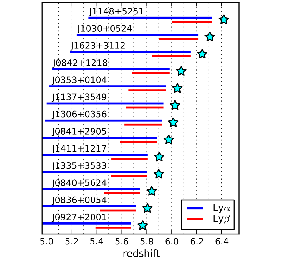
Our sample consists of 13 quasars at with spectroscopy from the Echellette Spectrograph and Imager (ESI; Sheinis et al., 2002) on the Keck II telescope (Table 1). We use only ESI spectra in order to have uniform wavelength coverage and resolution, and also for the high signal-to-noise ratio () even in relatively short exposures. Details of the reduction procedures are given in White et al. (2003). Most of these spectra were included in Fan et al. (2006); as in that work we exclude quasars with broad absorption line (BAL) features. The quasar redshifts have been updated to match the values given in Carilli et al. (2010), taking advantage of more accurate CO and \textMg ii redshifts when available. The spectra have widely varying exposure times (from 15 minutes to hours) and span 1.8 optical magnitudes in flux, and thus have widely differing levels in the Lyman forest regions.
We quantify the dynamic range of each spectrum in terms of the average limiting optical depth in the Ly and Ly forests. To derive these quantities, we fit the power-law continuum model for the rest-frame UV from Telfer et al. (2002) to the unabsorbed continuum redward of Ly. The average limiting optical depths in the Ly forest are then calculated as and shown in Table 1. For the Ly forest the continuum flux, and hence dynamic range, is affected by absorption from the underlying 4–5 Ly forest, as the photons redshift into Ly resonance at . We account for this effect using the redshift evolution of the mean opacity given in Fan et al. (2006). On the other hand, the optical depth is reduced by the weaker oscillator strength () and shorter wavelength of Ly (), which increases the dynamic range in the Ly forest relative to Ly. Note that the continuum fitting and the derived optical depths are strictly used to characterize the quality of the spectra, and do enter into the classification of “dark” pixels, which is the main result of this work (see §3).
We bin the spectra into pixels of width 3.3 Mpc. The ESI spectra have a wavelength resolution of (Fan et al., 2006), though they are sampled at a higher resolution during extraction. Binning to 3.3 Mpc results in pixels with calculated from the mean of unbinned pixels. This increases the dynamic range by (as determined from the optical depth).444Our choice of pixel size is fairly arbitrary, and could be considered one of the few “model” uncertainties in this work. This scale is a factor of a few times the Jean’s length in the mean-density, ionized IGM. Furthermore, a simple estimate of the photoevaporation timescale of mean-density, 3 Mpc regions exposed to the observed mean (e.g., Bolton & Haehnelt, 2007b), yields . This suggests that even smaller \textH i patches could persevere for a non-trivial time. Neglecting such sub-pixel \textH i structure likely makes our results again more conservative, since the associated strong opacity in the core of the Lyman line, as well as a potentially strong contribution from the damping wings (e.g., Miralda-Escude, 1998), would likely cause the entire 3.3 Mpc “pixel” to be dark, resulting in an overestimate of the covering fraction. More generally. by absorbing flux in neighboring pixels, damping wing absorption from potential \textH i patches would make our upper limits more conservative. Unfortunately, estimating the impact of damping wings is highly model-dependent, requiring the distribution of \textH i impact parameters and partial ionization levels. In either case, we plan on combining our sky-noise-limited ESI spectra with read-noise-limited high-resolution HIRES spectra (e.g., Becker et al. 2007) in an attempt to resolve sub-structure. Note that we are not discussing collapsed structures (e.g., Iliev, Shapiro, & Raga, 2005), which are more appropriately labeled as LLSs or DLAs contributing to the absorption inside the ionized IGM component.
Though the ESI spectra have been degraded in resolution in order to increase the dynamic range, the higher native resolution of the spectra confines the strong night sky emission lines to relatively small scales. We take advantage of this property to select bins between the brightest sky lines. First, the average noise is calculated in a 3.3 Mpc window centered on each pixel in the unbinned spectrum. Minima in the average noise are identified, and bins are placed at these minima. This effectively identifies locations where binned pixels can “fit” between bright sky lines. Finally, the spaces between these bins are iteratively filled with additional bins located at the minima within the spaces until no more bins can fit. We then remove from our analysis any pixels with too low of a threshold in optical depth, defined as a limit of .
This process results in relatively uniform noise across the full wavelength range, without resorting to smoothing techniques that could amplify correlations between the pixels (e.g., White et al., 2003). In addition, most of the binned pixels are non-adjacent, further reducing the susceptibility of our calculations to correlated noise introduced during extraction of the 2D spectra, and also to any physical correlations within the IGM on scales corresponding to the bin size. In the following sections we use “pixel” to refer to a 3.3 Mpc binned pixel derived from this process.
Finally, we limit the wavelength ranges of the Lyman forests used in our analysis in order to avoid biases and contamination. The red edge of both the Ly and Ly forests is taken to be 40 Mpc from the quasar redshift (). This is roughly the minimum distance required to reduce bias from the quasar’s surrounding \textH ii morphology due to the local overabundance of clustered galaxies (Alvarez & Abel, 2007; Mesinger, 2010). The blue edge of the Ly forest is at , chosen to avoid wavelengths affected by emission from Ly and \textO vi (Fan et al., 2006), and contamination from the Ly forest. The blue edge of the Ly forest is at in order to avoid contamination from Ly emission and the Ly forest. We show the span of the Ly and Ly forests in Fig. 1 for all spectra used in our analysis.
3 Defining “Dark” Pixels
We now quantitatively define what we mean by a “dark” pixel. We apply two criteria, as defined below, to the Ly and Ly forests from our spectra. In addition, we note that dark pixels arising from a pre-overlap neutral region must be dark in both Ly and Ly. Therefore, where we have overlapping (in redshift, see Fig. 1) spectral coverage of Ly and Ly we also present the combined dark fractions.
We stress that neither method used to calculate the covering fraction of dark pixels directly relies on continuum fitting, and thus we are relatively insensitive to the significant uncertainties associated with this process.
3.1 Dark pixel fraction using a flux threshold
First, we define dark pixels using only the flux and noise properties of the spectra: a pixel is dark if it has flux , where is the measured flux and is the measured noise of each pixel. Simply put, a pixel is dark if it has a flux consistent with zero within the given (assumed Gaussian) noise, and is not dark if it has . We have adopted a threshold of . For this threshold, of dark pixels will be scattered above the threshold and misclassified; thus we augment our dark pixel counts and uncertainties by this amount. Additionally, pixels with fluxes just above the threshold can be scattered below it, making our upper limits slightly more conservative (modeling this minor effect would require knowledge of the underlying pixel flux distribution).
Our choice of a threshold is somewhat arbitrary. We compared results obtained with a threshold and found they are consistent – though understandably slightly weaker – with those presented below.
3.2 Dark pixel fraction using negative pixels
If the noise in the extracted ESI spectrum is symmetric about zero, pixels that intrinsically have zero flux will have equal probabilities to be scattered into positive and negative values. Therefore, we can also estimate the number of dark pixels by simply counting pixels with negative flux and multiplying by two. Again, some pixels with small positive fluxes will be scattered to negative fluxes and thus incorrectly counted as dark, but this effect should be even smaller than when using the flux threshold method.
When we present the combined dark fraction from redshift-overlapping Ly and Ly forests, we multiply the number of instances of negative flux in both Ly and Ly by a factor of four. Again, if the noise is symmetric about zero, then a pixel with intrinsic zero-flux will have a 1/4 chance of having observed negative fluxes in both Ly and Ly.
Counting dark pixels using negative values relies on the assumption that the noise is symmetrically distributed about zero for pixels with no intrinsic flux. Systematic effects in the reduction process, such as incorrect sky subtraction, could bias these values and hence our results. We do not see any evidence for this type of bias from examination of the pixel flux distribution 555For example, examination of the flux distributions in the forest regions normalized by the standard error shows that they are roughly Gaussian with and , ignoring the tail to positive flux values arising from flux leaks within the forest.. Additionally, the deeper spectra are less susceptible to this type of bias, as they are created by combining many individual exposures, averaging over such effects.
4 Ly/ forest examples
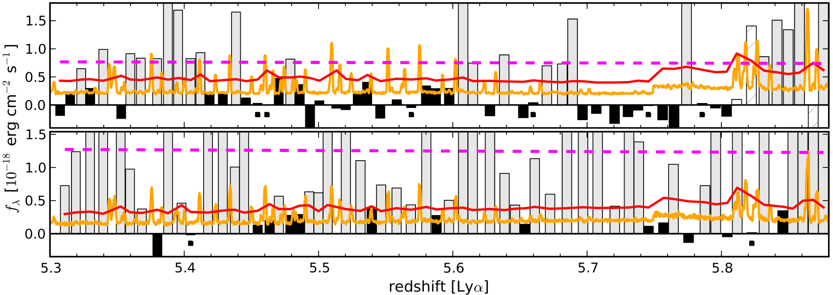
Figure 2 shows example Ly forests for two objects. The figure demonstrates the placement of bins away from bright sky lines and the relatively uniform noise in the binned pixels used for the final calculation of the dark pixel fraction. The forest for J0841+2905 is considerably darker than that of J1306+0356 in the same redshift range. This is likely a consequence of the lower dynamic range of the J0841+2905 spectrum, but there could also be contributions from line-of-sight variance. This highlights the need for both many lines-of-sight and high quality spectra when deriving constraints from the Ly forest.
The Ly forest yields a stronger constraint on the fraction of dark pixels, as the relative weakness of the Ly transition compared to Ly results in greater dynamic range. The specific ratio of varies from pixel-to-pixel depending on the sub-pixel structure of the IGM (e.g., Songaila, 2004; Fan et al., 2006), and the absorption from the underlying Ly forest (see §2). Since we are treating the dark fraction as a direct upper limit on , we do not introduce any model assumptions about either the clumpiness of the IGM at or the nature of the lower-redshift Ly forest into our results. In future work, we will attempt to resolve and model-out the underlying Ly forest from the Ly region, yielding tighter constraints, albeit at the cost of introducing model uncertainties (see §7).

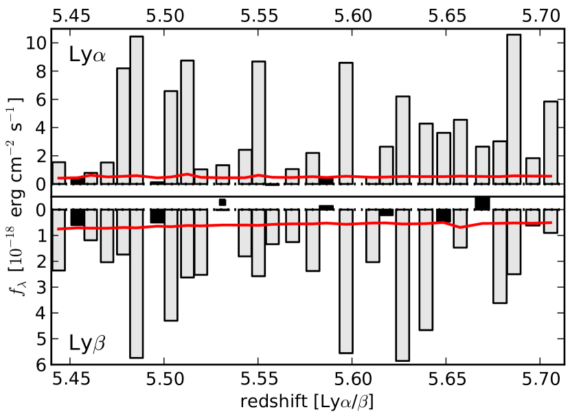
In Fig. 3, we show a comparison of the Ly and Ly forests for J0836+0054, overlayed in absorption redshift. The 2 noise level is shown with a red line, and dark pixels identified with this flux threshold (§3.1) are shown in black. As mentioned above, the contamination of the Ly by the lower-redshift Ly forest can result in dark pixels even when the corresponding pixels in Ly are not dark. Pixels corresponding to pre-overlap, highly neutral regions must be dark in both Ly and Ly. In this figure there are two such pixels. The intersection of dark pixels in both forests provides the strongest possible constraint available from this method; however, due to the limited dynamic range the presence of dark pixels in both forests is a necessary but not sufficient indication of neutral IGM.
Finally, it is important to remember that each of our pixels is a non-trivial 3.3 Mpc in size. As already discussed, a single dark pixel is sufficiently large to be a potential tracer of pre-overlap HI, especially when weighted by the LOS impact parameter. In fact, extended dark patches need not be a good tracer of reionization in high-redshift spectra, especially when the spectra begin to saturate (Mesinger, 2010).
5 Results
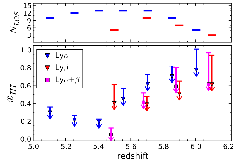
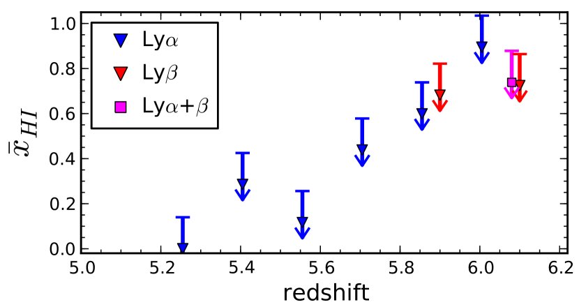
The main results of this work are presented in Fig. 4. The covering fractions of dark pixels computed using the flux threshold (§3.1) and negative pixel (§3.2) statistics are directly converted into a upper limit666As mentioned previously, in addition to any possible pre-overlap \textH i, the dark pixel fraction also includes contributions from \textH i embedded in the ionized IGM with an optical depth greater than the available dynamic range; hence it is only an upper limit on . Additionally, partially ionized neutral IGM (see discussion in §6) and unresolved ionization substructure (on scales smaller than our pixels) make our upper limits even more conservative. on the neutral hydrogen fraction and shown in the bottom left and right panels, respectively. The dark fractions calculated from the Ly, Ly, and combined Ly + Ly forests are shown in blue, red, and magenta, respectively. Pixels are binned in redshift bins of 0.15 (0.2) for the Ly (Ly) forest777Wide redshift bins decrease the sample variance, but also average over any IGM evolution. Our fiducial bin choice (although fairly arbitrary) is narrower than the likely reionization time-scales: Hubble time, photoevaporation time of pixel-sized regions, and the growth of the halo mass function (see, e.g., Fig. 9 in Mesinger, Johnson, & Haiman 2006 and Fig. 1 in Lidz et al. 2007). Therefore, our bins are likely narrow enough to resolve cosmic evolution, and wide enough to have decent sampling of the (possible) reionization morphology in the regime (see §6).. The upper left panel shows the number of pixels in each redshift bin, and the upper right panel shows the number of independent lines-of-sight contributing to each bin.
The fraction of dark pixels in each bin and the associated uncertainty on this fraction are obtained using the jackknife method. We repeat the calculation 13 times, each time leaving out one of the spectra. We then use jackknife statistics to derive the mean and variance from the fractions calculated during each resampling888Note that this is not a strict application of the jackknife method, as leaving out one spectrum at a time results in a varying number of pixels in each resampling. However, this variation is small.. Since the dark fraction is an upper limit on , the derived variance is shown only in the upper limits of Figure 4. Jackknife errors may or may not fully capture the variance inherent to the reionization process; in any case, we estimate such cosmic variance to be small for our full sample (see §6). Rather, the sample variance is most likely dominated by the disparate dynamic ranges of the spectra.
Using the flux threshold (negative pixel) method, we find upper limits of at (fairly independent of redshift), increasing to at . As expected, the most powerful constraint for the flux threshold method is obtained from the combined Ly and Ly forests, by requiring that overlapping pixels in both forests are dark999Note that the bins used in the analysis of the Ly, Ly, and Ly + Ly forests as shown in Fig. 4 are offset in redshift. Therefore the sample variance between the bins can result in a Ly + Ly dark fraction which is slightly higher than one obtained just from the Ly, as is the case for the last set of points in the lower left panel.. The benefit of using the overlapping forests is not as evident for the negative pixel method, since it relies on events rarer by a factor of two (see §3.2), and so has intrinsically larger sample variance than using just a single forest. Including the 1- jackknife errors degrades the constraints by () for the flux threshold (negative pixel) method.
The two methods for estimating the dark covering fraction yield comparable results, though the negative flux method generally results in lower dark fractions. This could be due to many pixels with small positive flux levels contributing to the flux threshold method counts (§3.1). By pushing the threshold to flux many such pixels are eliminated, at the cost of higher sample variance.
There is a notable change in the evolution of the dark fraction at . This feature appears to be genuine and is due to the fact that dark gaps in several spectra terminate at this redshift. Although it might be tempting to suggest this feature could be due to reionization, such an interpretation is premature. There is no obvious, corresponding feature in the redshift evolution of (Songaila, 2004; Fan et al., 2006; Becker et al., 2007). Nevertheless, given the large scatter in the sample, and the difficulties in using as a reionization tracer, it will be worthwhile to investigate this feature with larger sample sizes and modeling.
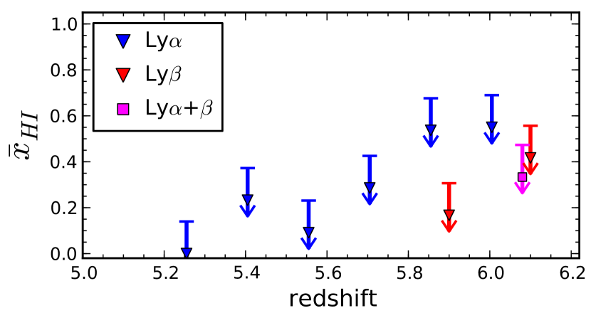
In Fig. 5, we present results using only our two deepest spectra (10 hour exposure times). These have an effective dynamic range of and 7-20 (see Table 1). With just the two deepest spectra, we obtain mean dark fractions of at and at , with the flux threshold (negative pixel) criteria.
Although these mean values are generally lower than those from our full sample (Fig. 4), they are also more susceptible to cosmic variance. Having two LOSs increases the fractional uncertainty in the sample mean by a factor of compared to our full sample of 13 LOSs, since the uncertainty in the sample mean scales with the number of samples as (see §6). This susceptibility to cosmic variance depends on , increasing as the neutral patches become rarer. Taking the specific case of from Fig. 6, we see that the uncertainty in the mean dark fraction (due to reionization) from two LOS segments of width is comparable to the mean. Reducing this uncertainty requires more deep spectra in order to take full advantage of the increased dynamic range.
Even with this model-dependent, though conservative, choice of cosmic variance error bars, our deepest two spectra yield at , comparable with those obtained from the full sample. Furthermore, using the negative pixel criteria in the right panel of Fig. 5, we are able to place a robust upper limit at of .
Several model-dependent constraints on reionization at have been derived from other astrophysical probes such as: (1) the size of the proximity zone around quasars (Wyithe, Loeb, & Carilli 2005; Fan et al. 2006; Carilli et al. 2010, but see Mesinger, Haiman, & Cen 2004; Bolton & Haehnelt 2007; Maselli et al. 2007); (2) a claimed detection of damping wing absorption from neutral IGM in quasar spectra (Mesinger & Haiman 2004, 2007, but see Mesinger & Furlanetto 2008); (3) the non-detection of intergalactic damping wing absorption in a gamma ray burst spectrum (Totani et al. 2006, but see McQuinn et al. 2008); and (4) the number density and clustering of Ly emitters (Malhotra & Rhoads 2004; Haiman & Cen 2005; Furlanetto, Zaldarriaga, & Hernquist 2006; Kashikawa et al. 2006; McQuinn et al. 2007, but see Dijkstra, Wyithe, & Haiman 2007; Mesinger & Furlanetto 2008b; Iliev et al. 2008, Dijkstra, Mesinger, & Wyithe, in preparation). All of these constraints are controversial, with considerable uncertainties. Our limit of is comparable to or better than these existing upper limits, and is much more robust (the model-dependence comes in the form of the cosmic variance error bar, and our choice here is conservative).
At lower redshifts (), previous claims of a highly-ionized IGM (–; e.g., Fig. 7 in Fan et al. 2006) are derived under the a priori assumption of a uniform background. Given that reionization by stellar sources is highly inhomogenous, this carries the implicit assumption that reionization is over, and therefore the standard conversion cannot be used to place direct constraints on reionization, even with complete confidence in the density distribution of the IGM. The upper limits we present in Fig. 4 are the first direct, model-independent constraints on at these redshifts.
6 Cosmic Variance During Reionization
The jackknife error bars in Fig. 4 show the sightline-to-sightline standard deviation in the dark pixel fraction measured from our observational sample. The main source of this variation is the disparate dynamic range of our spectra. However, the covering fraction of dark pixels itself can intrinsically vary from sightline-to-sightline. Again, this dark fraction has a contribution from the ionized IGM and potentially the pre-overlap neutral IGM. Since this paper places upper limits on , we concern ourselves with the cosmic variance of the latter, i.e., reionization.
During the final stages of reionization, the pre-overlap neutral regions become increasingly rare. If the mean spacing of the neutral islands is comparable to or greater than the length of our LOS segments, then our sample is prone to cosmic variance, and we would need many LOSs to have robust constraints on . This intrinsic cosmic variance might not be included in empirically derived jackknife error bars. To lessen the cosmic variance, one could extend the size of the LOS segments (i.e. redshift bins), but then one is averaging over redshift evolution.
Here we try to get a rough, quantitative estimate of the number of LOSs required for an accurate sampling of pre-overlap \textH i. We note that this is a highly model-dependent estimate and so a detailed treatment is not appropriate for this work. We begin by noting that the covering fraction of neutral IGM during reionization, computed from an ensemble of LOS segments, can be thought of as sampling some fundamental distribution with mean ,101010Note that since the “neutral” IGM during reionization could be partially ionized, the mean covering fraction, , does not have to equal , but can be larger. Because of the strength of the Lyman series transitions, the covering fraction statistic does not distinguish between partially ionized \textH i regions, , and those which are fully neutral, . However, the mean neutral fraction, , does care if regions are partially or fully ionized. Note that here we are only referring to the “neutral” IGM, not the residual \textH i in the ionized IGM, which should be at the level of (e.g., Bolton & Haehnelt, 2007b). For example, in the fiducial model of Mesinger (2010), for we obtain . Therefore, we differentiate between the covering fraction of neutral IGM and . We caution the reader that this difference is highly model dependent. and standard deviation, . According to the central limit theorem, as the sample size increases, the sample average of the covering fraction of neutral IGM approaches a normal distribution with mean and standard deviation, .
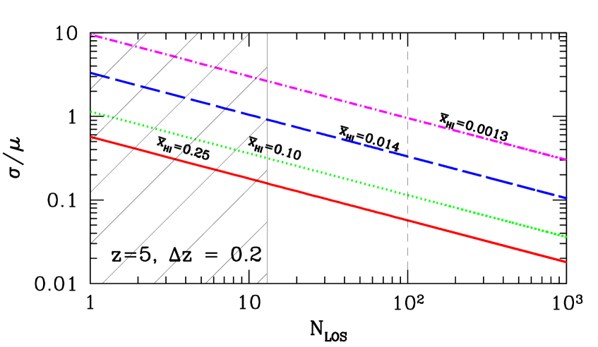
In Fig. 6, we plot the fractional uncertainty, , of the mean covering fraction of neutral IGM obtained from samples. The standard deviation of the single sample (i.e. from 1 LOS) distribution of the \textH i covering fraction, , is taken from the fiducial models of Mesinger (2010)111111These reionization morphologies are created with the publicly available, semi-numerical simulation DexM: http://www.astro.princeton.edu/~mesinger/Sim.html. Simulation boxes are 2 Gpc on a side with 3 Mpc cells. In the fiducial models, suites of reionization morphologies are created at a fixed redshift by varying the ionization efficiencies of atomically-cooled (M) sources, with an assumed attenuation length inside the ionized IGM of 50 Mpc.. All curves are computed at and assume LOS segments of length , roughly corresponding to the bin size we use in this work. Roughly speaking, the curves indicate how many LOS segments are required such that their average covering fraction is close to the true value within the given fractional uncertainty.
The shaded region in Fig. 6 corresponds to the sample used in this work (see the top, right panel of Fig. 4). This means that at , where we have a sample size of , we can be reasonably certain that our sampling of pre-overlap \textH i is accurate to better than 50% of the true value, if the true value is (i.e., a significantly neutral Universe). Of course, if the Universe is more ionized, the neutral IGM patches are rarer, and thus more LOSs are needed to obtain the same fractional uncertainty in their sample mean. For example, obtaining comparable accuracy for requires LOSs, which is just out of reach of the current published set of spectra, given that their forests do not all overlap121212Of course constraining to percent level precision with the Lyman forest is difficult to imagine, and so this discussion is mostly academic.. However, when the neutral patches are that rare, the dark covering fraction statistic is dominated by the ionized IGM, and is a very poor probe of reionization (Mesinger, 2010).
Constraints derived from our two deepest spectra (Fig. 5) are more susceptible to cosmic variance than those derived from our full sample. The fractional uncertainty in the mean value of the covering fraction of neutral IGM is a factor of 2.5 higher for two of our spectral segments than for 13. From Fig. 6, we see that for two spectra at , the standard deviation of the sample average is a factor times the mean value of , i.e. . For illustrative purposes, we use these estimates of the cosmic variance uncertainty for our dark fraction points in Fig. 5. Note that these error bars are model-dependent theoretical estimates, unlike the empirical jackknife errors shown for our full sample in Fig. 4, where cosmic variance was less problematic.
The error bars in Fig. 5 are appropriate for the covering fraction of neutral IGM, which can be substantially higher than , due to partial ionizations. In keeping with the conservative spirit of this work, we do not convert from the covering fraction to even in the error bars, making them overestimates of the uncertainty on .
7 Future work
The simple upper limit on obtained from this study is limited by contamination from absorption within the ionized IGM. This contamination can be addressed on two fronts: improved observations and theoretical modeling.
The observations can be improved by increasing the dynamic range of the pixels in order to eliminate pixels with intermediate absorption levels. Figure 5 shows that very deep spectra can strengthen the constraint by a factor of two; however, obtaining deep spectra is highly costly in telescope time, and the payoff in dynamic range with exposure time rises only as . In addition, the Ly forest provides a stronger constraint than Ly, but has a much shorter redshift path, and thus the amount of overlapping Ly forest between quasars at a range of redshifts grows slowly with the number of objects (note there is only one redshift bin for Ly+Ly in Fig. 5). An intermediate approach of obtainining a few hours of integration time on many objects seems better: balancing the needs for depth to detect intermediate absorption and for many independent lines-of-sight to reduce cosmic variance. This program can be accomplished with the sample of bright () quasars at available today.
Aside from increasing the sample of deep spectra, there are several complementary observations that can improve these dark fraction constraints. Higher resolution spectra, for example the HIRES sample of Becker et al. (2007), can be used to resolve flux leaks from dark pixels on smaller spatial scales. Additionally, one can use corresponding near-IR spectra (which we are in the process of collecting) to detect metal absorption corresponding to contaminating DLAs in the Ly/ forests, and remove their contribution from the dark pixel analysis.
In addition to the observations, one could also model the expected contribution of the ionized IGM to the dark fraction. Models can be calibrated using the latest data: (i) analytic/numeric models of the density field (e.g., Miralda-Escudé, Haehnelt, & Rees, 2000; Trac & Cen, 2007; Bolton & Becker, 2009); (ii) conservative (e.g., unevolving) extrapolations of the ionization rate from lower redshifts, where the ionization rate is very homogeneous and the Ly forest is well resolved (e.g., Croft, 2004; Bolton et al., 2006; Faucher-Giguère et al., 2008); and (iii) conservative extrapolations of the evolution of LLSs (Storrie-Lombardi et al., 1994; Stengler-Larrea et al., 1995; Péroux et al., 2003; Prochaska, O’Meara, & Worseck, 2010; Songaila & Cowie, 2010) These approaches can be used to estimate the covering fraction of dark pixels expected from the ionized IGM and its redshift evolution. Removing this contamination from the total dark pixel counts leads to a model-dependent constraint on . With sufficiently high quality data and robust limits on the ionized IGM contribution from models, the method presented here could be used to detect reionization if indeed a substantial neutral fraction remains at .
Furthermore, Fig. 5 demonstrates the power of high dynamic range spectra from very deep observations within the regime where the IGM saturates absorption spectra. A greater dynamic range aids in detecting flux from the ionized IGM (except for high column density systems such as LLSs), but not the neutral IGM as it is far beyond the achievable range. Hence the rate of change of the dark fraction as a function of the spectral dynamic range can provide an interesting constraint on . Comparing this rate of change with the slope of an assumed density PDF could yield model-dependent constraints on reionization. If, for example, the dark fraction was observed to converge towards a constant value with increasing dynamic range (beyond what could be attributed to high column density systems), that would be a reionization signpost. We defer more detailed analysis to future work.
8 Conclusions
We present upper limits on the neutral hydrogen fraction at derived from the simple, robust statistic of the covering fraction of dark pixels in the Ly/ forests of high redshift quasars. The interpretation of quasar absorption spectra is complicated by the inhomogeneous nature of reionization and the finite dynamic range of the Lyman forests: dark spectral regions can result either from residual \textH i in the ionized IGM, or from pre-overlap neutral patches during the epoch of reionization. By conservatively associating all dark patches with pre-overlap \textH i, we provide a constraint that is nearly model-independent.
Using a sample of 13 quasars with Keck ESI spectra, we constrain the neutral fraction to be at , rising to at . We find evidence of a break in the redshift evolution of the dark covering fraction at . Previous claims of a highly-ionized IGM at these redshifts (–; e.g., Fig. 7 in Fan et al. 2006) are derived under the a priori assumption of a uniform background. Given that reionization by stellar sources is highly inhomogeneous, this carries the implicit assumption that reionization is over, and therefore the standard conversion cannot be used to place direct constraints on reionization, even with complete confidence in the density distribution of the IGM.
At , more stringent constraints are provided by the subsample of our two deepest spectra when combined with conservative, albeit model-dependent, estimates of cosmic variance. Specifically, we obtain . When re-evaluated in the context of an inhomogeneous reionization, the existing constraints on (derived from QSO proximity regions, damping wings in QSO and GRB spectra, LAE number density and clustering properties) are sensitive probes only of the early stages of reionization, when the Universe was mostly neutral. Additionally, they are highly model-dependent. Our constraint of is comparable to or better than these existing constraints, and is much more robust.
We expect these limits to improve with a larger sample of deep spectra. The dark covering fraction statistic can also be combined with theoretical estimates of the absorption inside the ionized IGM to yield a model-dependent constraint. Finally, the rate of change of the dark fraction as a function of the spectral dynamic range can provide an interesting constraint on . We will explore these possibilites in future work.
Our results show that present-day observations of Lyman forest absorption in quasars do not rule out an end to reionization as late as ; thus the generic statement that reionization completes by is unjustified. Indeed, the tail end of reionization could stretch to without a strong observational imprint, since the final stages of reionization – when the UVB became regulated by LLSs and their evolution (Furlanetto & Mesinger, 2009; Crociani et al., 2010) – may have been extended (Furlanetto & Oh, 2005; Alvarez & Abel, 2010).
The goal of this work is not to promote a late reionization scenario. We simply note that it is not ruled out by current data, and caution against further unjustified leaps of interpretation. We present a direct, conservative upper limit on that does not rely on any assumptions about the quasar continuum, IGM density, \textH ii morphology or ionizing background fields. This can be viewed as a robust starting point for interpretations of high-redshift observations and theoretical models.
We thank George Becker and Matthew McQuinn for useful
discussions and comments on a draft version of this paper. We acknowledge the
efforts of Bob Becker and Rick White to collect and reduce the Keck data
presented here.
IDM and XF are supported by a Packard Fellowship for Science and Engineering
and NSF grant AST 08-06861.
AM is supported by NASA through Hubble Fellowship grant
HST-HF-51245.01-A, awarded by the Space Telescope Science Institute, which is
operated by the Association of Universities for Research in Astronomy, Inc.,
for NASA, under contract NAS 5-26555.
This work made use of the CosmoloPy package (http://roban.github.com/CosmoloPy/).
The authors wish to recognize and acknowledge the very significant cultural role
and reverence that the summit of Mauna Kea has always had within the indigenous
Hawaiian community. We are most fortunate to have the opportunity to conduct
observations from this mountain.
Facilities: Keck:II (ESI)
References
- Alvarez & Abel (2007) Alvarez, M. A., & Abel, T. 2007, MNRAS, 380, L30
- Alvarez & Abel (2010) Alvarez, M. A., & Abel, T. 2010, arXiv:1003.6132
- Becker et al. (2001) Becker, R. H., et al. 2001, AJ, 122, 2850
- Becker et al. (2007) Becker, G. D., Rauch, M., & Sargent, W. L. W. 2007, ApJ, 662, 72
- Bolton & Becker (2009) Bolton, J. S., & Becker, G. D. 2009, MNRAS, 398, L26
- Bolton & Haehnelt (2007) Bolton, J. S., & Haehnelt, M. G. 2007, MNRAS, 374, 493
- Bolton & Haehnelt (2007b) Bolton, J. S., & Haehnelt, M. G. 2007b, MNRAS, 382, 325
- Bolton et al. (2006) Bolton, J. S., Haehnelt, M. G., Viel, M., & Carswell, R. F. 2006, MNRAS, 366, 1378
- Busha et al. (2010) Busha, M. T., Alvarez, M. A., Wechsler, R. H., Abel, T., & Strigari, L. E. 2010, ApJ, 710, 408
- Carilli et al. (2010) Carilli, C. L., et al. 2010, ApJ, 714, 834
- Choudhury et al. (2008) Choudhury, T. R., Ferrara, A., & Gallerani, S. 2008, MNRAS, 385, L58
- Crociani et al. (2010) Crociani, D., Mesinger, A., Moscardini, L., & Furlanetto, S. 2010, arXiv:1008.0003
- Croft (2004) Croft, R. A. C. 2004, ApJ, 610, 642
- de Rosa et al. (2011) de Rosa, G., et al. 2011, submitted
- Dijkstra et al. (2004) Dijkstra, M., Haiman, Z., & Loeb, A. 2004, ApJ, 613, 646
- Dijkstra et al. (2007) Dijkstra, M., Wyithe, J. S. B., & Haiman, Z. 2007, MNRAS, 379, 253
- Djorgovski et al. (2001) Djorgovski, S. G., Castro, S., Stern, D., & Mahabal, A. A. 2001, ApJ, 560, L5
- Dunkley et al. (2009) Dunkley, J., et al. 2009, ApJS, 180, 306
- Fan et al. (2004) Fan, X., et al. 2004, AJ, 128, 515
- Fan et al. (2001) Fan, X., et al. 2001, AJ, 122, 2833
- Fan et al. (2002) Fan, X., Narayanan, V. K., Strauss, M. A., White, R. L., Becker, R. H., Pentericci, L., & Rix, H.-W. 2002, AJ, 123, 1247
- Fan et al. (2006) Fan, X., et al. 2006b, AJ, 132, 117
- Fan et al. (2006b) Fan, X., et al. 2006c, AJ, 131, 1203
- Fan et al. (2003) Fan, X., et al. 2003, AJ, 125, 1649
- Faucher-Giguère et al. (2008) Faucher-Giguère, C.-A., Lidz, A., Hernquist, L., & Zaldarriaga, M. 2008, ApJ, 682, L9
- Furlanetto & Mesinger (2009) Furlanetto, S. R., & Mesinger, A. 2009, MNRAS, 394, 1667
- Furlanetto & Oh (2005) Furlanetto, S. R., & Oh, S. P. 2005, MNRAS, 363, 1031
- Furlanetto et al. (2004) Furlanetto, S. R., Zaldarriaga, M., & Hernquist, L. 2004, ApJ, 613, 1
- Furlanetto et al. (2006) Furlanetto, S. R., Zaldarriaga, M., & Hernquist, L. 2006, MNRAS, 365, 1012
- Gnedin (2000) Gnedin, N. Y. 2000, ApJ, 535, 530
- Goto (2006) Goto, T. 2006, MNRAS, 371, 769
- Gunn & Peterson (1965) Gunn, J. E., & Peterson, B. A. 1965, ApJ, 142, 1633
- Haiman & Cen (2005) Haiman, Z., & Cen, R. 2005, ApJ, 623, 627
- Iliev et al. (2008) Iliev, I. T., Shapiro, P. R., McDonald, P., Mellema, G., & Pen, U.-L. 2008, MNRAS, 391, 63
- Iliev et al. (2005) Iliev, I. T., Shapiro, P. R., & Raga, A. C. 2005, MNRAS, 361, 405
- Jiang et al. (2008) Jiang, L., et al. 2008, AJ, 135, 1057
- Kashikawa et al. (2006) Kashikawa, N., et al. 2006, ApJ, 648, 7
- Kohler & Gnedin (2007) Kohler, K., & Gnedin, N. Y. 2007, ApJ, 655, 685
- Komatsu et al. (2009) Komatsu, E., et al. 2009, ApJS, 180, 330
- Lidz et al. (2007) Lidz, A., McQuinn, M., Zaldarriaga, M., Hernquist, L., & Dutta, S. 2007, ApJ, 670, 39
- Lidz et al. (2006) Lidz, A., Oh, S. P., & Furlanetto, S. R. 2006, ApJ, 639, L47
- Malhotra & Rhoads (2004) Malhotra, S., & Rhoads, J. E. 2004, ApJ, 617, L5
- Maselli et al. (2007) Maselli, A., Gallerani, S., Ferrara, A., & Choudhury, T. R. 2007, MNRAS, 376, L34
- McQuinn et al. (2007) McQuinn, M., Hernquist, L., Zaldarriaga, M., & Dutta, S. 2007, MNRAS, 381, 75
- McQuinn et al. (2007b) McQuinn, M., Lidz, A., Zahn, O., Dutta, S., Hernquist, L., & Zaldarriaga, M. 2007b, MNRAS, 377, 1043
- McQuinn et al. (2008) McQuinn, M., Lidz, A., Zaldarriaga, M., Hernquist, L., & Dutta, S. 2008, MNRAS, 388, 1101
- Mesinger (2010) Mesinger, A. 2010, MNRAS, 407, 1328
- Mesinger & Dijkstra (2008) Mesinger, A., & Dijkstra, M. 2008, MNRAS, 390, 1071
- Mesinger et al. (2004) Mesinger, A., Haiman, Z., & Cen, R. 2004, ApJ, 613, 23
- Mesinger & Furlanetto (2007) Mesinger, A., & Furlanetto, S. 2007, ApJ, 669, 663
- Mesinger & Furlanetto (2008) Mesinger, A., & Furlanetto, S. R. 2008, MNRAS, 385, 1348
- Mesinger & Furlanetto (2008b) Mesinger, A., & Furlanetto, S. R. 2008b, MNRAS, 386, 1990
- Mesinger & Furlanetto (2009) Mesinger, A., & Furlanetto, S. 2009, MNRAS, 400, 1461
- Mesinger & Haiman (2007) Mesinger, A., & Haiman, Z. 2007, ApJ, 660, 923
- Mesinger & Haiman (2004) Mesinger, A., & Haiman, Z. 2004, ApJ, 611, L69
- Mesinger et al. (2006) Mesinger, A., Johnson, B. D., & Haiman, Z. 2006, ApJ, 637, 80
- Miralda-Escude (1998) Miralda-Escude, J. 1998, ApJ, 501, 15
- Miralda-Escudé et al. (2000) Miralda-Escudé, J., Haehnelt, M., & Rees, M. J. 2000, ApJ, 530, 1
- Péroux et al. (2003) Péroux, C., McMahon, R. G., Storrie-Lombardi, L. J., & Irwin, M. J. 2003, MNRAS, 346, 1103
- Prochaska et al. (2010) Prochaska, J. X., O’Meara, J. M., & Worseck, G. 2010, ApJ, 718, 392
- Sheinis et al. (2002) Sheinis, A. I., Bolte, M., Epps, H. W., Kibrick, R. I., Miller, J. S., Radovan, M. V., Bigelow, B. C., & Sutin, B. M. 2002, PASP, 114, 851
- Songaila (2004) Songaila, A. 2004, AJ, 127, 2598
- Songaila & Cowie (2002) Songaila, A., & Cowie, L. L. 2002, AJ, 123, 2183
- Songaila & Cowie (2010) Songaila, A., & Cowie, L. L. 2010, ApJ, 721, 1448
- Stengler-Larrea et al. (1995) Stengler-Larrea, E. A., et al. 1995, ApJ, 444, 64
- Storrie-Lombardi et al. (1994) Storrie-Lombardi, L. J., McMahon, R. G., Irwin, M. J., & Hazard, C. 1994, ApJ, 427, L13
- Telfer et al. (2002) Telfer, R. C., Zheng, W., Kriss, G. A., & Davidsen, A. F. 2002, ApJ, 565, 773
- Totani et al. (2006) Totani, T., Kawai, N., Kosugi, G., Aoki, K., Yamada, T., Iye, M., Ohta, K., & Hattori, T. 2006, PASJ, 58, 485
- Trac & Cen (2007) Trac, H., & Cen, R. 2007, ApJ, 671, 1
- Trac & Gnedin (2009) Trac, H., & Gnedin, N. Y. 2009, arXiv:0906.4348
- Volonteri & Gnedin (2009) Volonteri, M., & Gnedin, N. Y. 2009, ApJ, 703, 2113
- White et al. (2003) White, R. L., Becker, R. H., Fan, X., & Strauss, M. A. 2003, AJ, 126, 1
- Willott et al. (2010) Willott, C. J., et al. 2010, AJ, 139, 906
- Wyithe et al. (2005) Wyithe, J. S. B., Loeb, A., & Carilli, C. 2005, ApJ, 628, 575
- Zahn et al. (2010) Zahn, O., Mesinger, A., McQuinn, M., Trac, H., Cen, R., & Hernquist, L. E. 2010, arXiv:1003.3455