Abstract

Given that it will take quite some time for the Large Hadron Collider (LHC) to reach its desired luminosity, it is important to investigate the most favorable scenario in which supersymmetry (SUSY) may be discovered at the early runs at the LHC. Our aim in this work is to find such a scenario within the gravity mediated SUSY breaking (SUGRA) framework and select a class of final states that warrant a discovery at the very early runs of the LHC. It turns out that such a situation can be associated with a scenario where gluinos are sufficiently light and so are the third generation scalars while the first two family scalars are heavy. We find that this can be achieved from a high-scale set-up with scalar mass non-universality in the third family and gaugino mass non-universality with $M_{3}<M_{1},M_{2}$. We show that the final state channels which are most favorable in such a region of parameter space are $4b+{E_{T}}\!\!\!\!/$, $4b+\ell+{E_{T}}\!\!\!\!/$ and $2b+2\ell+{E_{T}}\!\!\!\!/$. We also justify our claim by comparing the results with a minimal supergravity (mSUGRA) scenario with similar gluino mass.

1 Introduction

With the Large Hadron Collider (LHC) already collected data for the run with a center-of-mass energy $E_{CM}$=7 TeV, the search for physics beyond the Standard Model has reached a new height of excitement. Supersymmetry (SUSY) has been one of the most popular scenarios in this category, due to its attractive theoretical framework and variety of phenomenological features it incorporates. Apart from stabilizing the Higgs sector, it also provides with a cold dark matter candidate in form of the lightest SUSY particle (LSP) with $R$-parity (${(-1)}^{3B+L+2S}$) conservation [1, 2] .

Out of different SUSY-breaking models, the most popular one is the minimal supergravity or mSUGRA [3]. Here all the SUSY-breaking parameters are derived from four and half parameters, namely, the universal gaugino mass ($M_{1/2}$), the universal scalar mass ($m_{0}$), the universal trilinear coupling ($A_{0}$) all at the GUT scale, $\tan\beta$, the ratio of the vacuam expectation values (vev) of the two Higgses and the sign of SUSY-conserving Higgsino mass parameter $\mu$. However, proposals have been made to go beyond the universality of scalar [4, 5, 6, 7, 8, 9, 10, 11, 12] and gaugino masses [13, 14] within the SUGRA framework itself, which are strongly motivated from supersymmetric Grand Unified Theory (SUSY-GUT) and low energy phenomenological constraints, for example, suppression of the flavor changing neutral current (FCNC) or CP-violation.

With the prospect of LHC running at $E_{CM}$= 14 TeV, it is quite likely to shed light upon SUSY if it exists at the TeV scale. Whether this is possible, and if at all, then when and how, depend strictly on the SUSY spectra that nature has chosen for us. The most likely manifestation of SUSY will be the excess in certain final state channels over the standard model (SM) background fluctuations.

Following this, the main trends of the phenomenological studies in search of SUSY in context of the LHC have been directed either to a model-based approach where one has a specific SUSY model under consideration and then to study the consequences in a collider, or to interpret the measured excess in signals to extract the SUSY- parameters such as mass, spin etc. using kinematic variables and/or distributions [15]. There have been efforts to study the so-called ‘LHC inverse problem’ [16] as well. While all these are very important and of absolute necessity at the same time, perhaps a combined knowledge of all such studies may provide us with the most useful hint to unravel SUSY at the upcoming collider experiment.

In this work, we try to address a relatively simple question - what is the most favorable supersymmetric spectra allowed by all the search limits and low energy constraints that can leave its imprint during the early run of the LHC and correspondingly what are the final states that are favorable for such a spectra. Our approach here is pragmatic, particularly from the experimental point of view, as well as, somewhat model independent to start with. We of course, associate our proposed spectra to a SUGRA pattern to justify our claim.

The answer to the question raised here, may look very simple at the first sight: have the minimum possible values of all SUSY particle masses allowed by current bounds. However, such a choice may not be consistent with a SUSY breaking scenario. We argue that a spectra with light gluinos, light third family scalars, but relatively heavy first two families (that can be derived from a high-scale non-universal SUGRA pattern), is one of the most favorable cases for the SUSY to be discovered at the early LHC runs. It is even more true when we look for the final states in form of $4b+{E_{T}}\!\!\!\!/$, $4b+\ell+{E_{T}}\!\!\!\!/$ and $2b+2\ell+{E_{T}}\!\!\!\!/$ as these arises from the decays of the dominant SUSY production processes in such a region of parameter space and have little contribution from the SM background. To prescribe these as the golden modes for early SUSY discovery, we of course, assume that the machine is tuned properly to measure missing energy and tag $b$-jets. This is also justified because the main characteristic of SUSY-signature is high missing energy which is carried away by the LSP in the $R$-parity conserving framework.

We see that, in order to keep the third family squarks much lighter than the first two, in our proposed benchmark scenario and to associate them with a SUGRA pattern, we require a scalar non-universality at high scale. On the other hand, to keep gluinos light and low-lying electroweak gauginos above the LEP limit at the same time, we require a gaugino mass non-universality with a heirarchy of $M_{3}<M_{1},M_{2}$ at the high scale. The gaugino mass non-universality of the form $M_{3}<M_{1},M_{2}$ is achievable within the framework of the SUSY-GUT [13, 14], while a scalar non-universality of such kind can be motivated from string-inspired models with flavor dependent couplings to the modular fields [17, 18]. To justify our claim, we also compare our results with a mSUGRA parameter point that gives similar gluino mass.

Our paper is organized as follows. In Section 2, we discuss the model under consideration and the selected benchmark points chosen for further studies concerning collider signatures. In Section 3, we discuss the final states that we look for, the details of the collider simulation strategy adopted here and the numerical results obtained from this analysis. We conclude in Section 4.

2 Model, Formalism and Benchmark Points

In this section we first advocate the favorable SUSY spectra under consideration. We also motivate the final state signals in which such a parameter space can be better observed. Then we show that such a spectra can be associated to a high-scale non-universal gaugino and scalar mass set-up in a GUT- based SUGRA framework. At the end of this section, we discuss the benchmark points chosen for studying the collider signals.

It is easy to appreciate that a scenario which claims to be favorable for discovery should have very light gluinos simply because it has a very high production rate at the LHC (gluinos are colour octets and the main production through gluons gets enhanced because of high gluon flux at this energy regime). What about the squarks ? If these are light, they also compete in production rate with the gluinos, given the fact that they also have strong interaction and comes with three families. In a generic sense, then light squarks are also favorable to add to the SUSY-final states. We need to remember also that the gluino dominantly decays through the on-shell squark-quark giving rise to more likely a jet-rich final state if first two generation squarks participate in the decay chain. The jetty final states have a large SM backgrounds coming from QCD processes. Associated leptons may arise in such cases, but, mostly from the decays of the electroweak gauginos that appear in the cascades in such situations. Increasing the possibility of final state leptons is better to see SUSY signals over the background fluctuations in a hadron collider machine. Although the situation with gluinos and squarks all being light, can in principle, warrant a discovery at the early run of LHC by suitable choice of event selection criteria, the question is can we think of something more distinctive? Actually we can exploit the fact that heavy quarks, namely the top and the bottom have the property of decaying to leptons or get identified by b-tagging itself. So, if the squarks belonging to the the first two generations be very heavy, then the gluinos will decay dominantly through sbottom-bottom or stop-top. While, with a similar sbottom and stop mass, the gluino is more likely to decay through sbottom-bottom simply because of the phase space. Both cases give rise to bottom quark rich final states. Then, if we look for the final states with multiple $b$s, namely, $4b+{E_{T}}\!\!\!\!/$, $4b+\ell+{E_{T}}\!\!\!\!/$ or $2b+2\ell+{E_{T}}\!\!\!\!/$, they capture the gluinos decaying through sbottom-bottom or stop-top, with the sbottom decaying through bottom-neutralino or a top-chargino and the stop decaying to top-neutralino or bottom-chargino. In each case, we expect bottom reach final state. Also contribution from stop and sbottom pair productions contribute to such kind of final states.

We discuss the final states with the cuts in details in Section 3.

From the model point of view, it also turns out that both FCNC and CP-violation constraints may be best tackled if one assumes the first two generations of scalars to be multi-TeV and (quasi-)degenerate in masses.  This so-called ‘inverted hierarchy’ is favored from low-energy constraints as well.

A scalar mass hierarchy of this sort can be achieved from a high-scale non-universality in first two family scalars with the third one. More specifically, if the squark masses get generated from two different uncorrelated mass parameters namely, ${m_{0}}^{3}$ and ${m_{0}}^{1,2}$ respectively for the third generation and first two generations at the high scale, then choosing a high value of ${m_{0}}^{1,2}$ and a small value of ${m_{0}}^{3}$, given a particular value of high scale gaugino mass parameter can yield a spectra of the pattern discussed above. Although, it is a phenomenological framework that we discuss here, it can be motivated from string inspired models with flavor dependent couplings to the modulaii fields [17, 18]. We would like to note that such a set up has been discussed early in some articles for studying the collider signature in context of the LHC [4, 12], but as mentioned early, not specifically in this context.

In order to have the gluinos as light as possible and at the same time the low-lying charginos and neutralinos above the threshold, we require a non-universality in gaugino masses to accommodate it in a SUGRA pattern. The hierarchy required at the high-scale is $M_{3}<M_{1},M_{2}$. This can be generated within the framework of SUSY-GUT with an underlying $SU(5)$ or $SO(10)$ gauge symmetry [13, 14]. Often one can incorporate a dimension five operator in the non-trivial extension of the gauge kinetic function $f_{\alpha\beta}(\Phi^{j})$ in terms of the non-singlet chiral superfields $\Phi^{N}$ of the form

$$Ref_{\alpha\beta}(\phi)F_{\mu\nu}^{\alpha}F^{\beta\mu\nu}=\frac{\eta(\Phi^{s})}{M}Tr(F_{\mu\nu}\Phi^{N}F^{\mu\nu})$$ (1)

where $\Phi^{N}$ belongs to the symmetric product of the adjoint representation of the underlying gauge group as

$$SU(5): (24\times 24)_{symm}=1+24+75+200$$ (2)

$$SO(10): (45\times 45)_{symm}=1+54+210+770$$

Gaugino masses become non-universal if the Higgses responsible for the GUT-breaking, belong to the possible non-singlet representations, unlike the minimal supergravity (mSUGRA) framework [13, 14]. Interestingly, the representations $75$ and $200$ belonging to $SU(5)$ or $770$ of $SO(10)$ break the GUT group to the SM, we obtain the required hierarchy of $M_{3}<M_{1},M_{2}$ at the GUT scale. We tabulate the non-universal gaugino mass ratios for these representations in Table 1. A linear combination of these non-singlet representations with the singlet one can yield the exact hierarchy that we use in the benchmark points. We would also like to mention that such a gaugino mass hierarchy is also supported from the dark- matter consideration, as the immediate effect of having a smaller $M_{3}$ yields a smaller $\mu$ after the RGE running, yielding a more Higgsino like lightest neutralino, which has much efficient annihilation rate to yield a consistent cold dark matter relic density.

Representation	$M_{3}:M_{2}:M_{1}$ at $M_{GUT}$
75 of $SU(5)$	1:3:(-5)
200 of $SU(5)$	1:2:10
770 of $SO(10)$: $H\rightarrow SU(4)\times SU(2)\times SU(2)$	1:(2.5):(1.9)

Table 1: Non-universal gaugino mass ratios for different non-singlet representations belonging to $SU(5)$ or $SO(10)$ GUT-group that gives rise to the hierarchy of $M_{3}<M_{1},M_{2}$ at the GUT scale.

Now we discuss the benchmark points chosen for the study of collider signature from this framework. We stick to have a high-scale universal $A_{0}$ set to zero. For all the points $sgn(\mu)$ has been taken to be positive and the Higgs mass parameters has been set equal to the third generation scalar masses $m_{H_{u}}^{2}=m_{H_{d}}^{2}={{m_{0}}^{3}}^{2}$. The values of $\tan\beta$ has been chosen such that it satisfies the experimental constraint branching ratio for the $b\longrightarrow s\gamma$ [19] which at the $3\sigma$ level is

$$2.77\times 10^{-4}<Br(b\rightarrow s\gamma)<4.33\times 10^{-4}.$$ (3)

Parameters are fine-tuned in a way that it gives a correct cold dark matter relic abundance. In cases it is smaller than the WMAP data [20], which at $3\sigma$ is

$$0.091<\Omega_{CDM}h^{2}<0.128\ ,$$ (4)

where $\Omega_{CDM}$ is the dark matter relic density in units of the critical density and $h=0.71\pm 0.026$ is the reduced Hubble constant (namely, in units of $100\ \rm km\ \rm s^{-1}\ \rm Mpc^{-1}$).

This leaves us with the opportunity for some other dark-matter component. As we mentioned earlier we compare our result with a mSUGRA point, which has a similar gluino mass. We denote the benchmark points as BP1, BP2 and BP3, while the mSUGRA point is denoted as MSG1. We tabulate the high-scale and low scale parameters in Table 2. BP2 has the lightest gluino among these and BP3 has the heaviest one.

Note that for BP3, we do not need a gaugino mass non-universality to keep the lighter chargino, neutralinos to rise above the experimental bound.

parameter	BP1	BP2	BP3	MSG1
$\tan\beta$	17	12	23	5
$(M_{3},M_{2},M_{1}$)	(140,180,180)	(125,250,250)	(153,153,153)	(200,200,200)
$({m_{0}}^{3},{m_{0}}^{1,2})$	(160,1000)	(160,1000)	(160,1000)	(70,70)
$A_{0}$	0	0	0	0
$sgn(\mu)$	+	+	+	+
$\mu$	166	123	190	285
$m_{\tilde{g}}$	389	349	421	495
$m_{\tilde{u}_{L}}$	1037	1034	1043	457
$m_{\tilde{t}_{1}}$	187	142	217	324
$m_{\tilde{t}_{2}}$	364	348	382	501
$m_{\tilde{b}_{1}}$	268	253	285	427
$m_{\tilde{b}_{2}}$	302	273	330	447
$m_{\tilde{e}_{L}}$	1005	1012	1003	159
$m_{{\tilde{\tau}}_{1}}$	157	178	138	107
$m_{{\tilde{\chi}_{1}}^{\pm}}$	104	98	98.5	132
$m_{{\tilde{\chi}_{2}}^{\pm}}$	223	244	233	317
$m_{\widetilde{\chi}_{4}^{0}}$	225	245	232	319
$m_{\widetilde{\chi}_{3}^{0}}$	178	135	203	291
$m_{\widetilde{\chi}_{2}^{0}}$	110	125	101	134
$m_{\widetilde{\chi}_{1}^{0}}$	64	71	56	73
$\Omega_{\tilde{\chi}_{1}}h^{2}$	0.08	0.035	0.128	0.128
$BF(b\to s\gamma)$	$3.04\times 10^{-4}$	$4.3\times 10^{-4}$	$4.27\times 10^{-4}$	$3.09\times 10^{-4}$

Table 2: : Benchmark points BP1, BP2, BP3 and MSG1(masses are in GeV). The first five parameters define the model, while the rest are low scale prediction.

For renormalization group equation RGE, we use the code SuSpect v2.3 [21] and stick to two-loop RGE with radiative corrections to the gauginos and squarks. We use full one loop and dominant two loop corrections for the Higgs mass. The low scale value of the strong coupling constant has been chosen at ${\alpha_{3}(M_{Z})}^{\overline{MS}}=0.1172$. We ensure radiative electroweak symmetry breaking and the electroweak symmetry breaking scale has been set at $\sqrt{m_{\tilde{t_{L}}}m_{\tilde{t_{R}}}}$, the default value in the code SuSpect. We compute the cold dark matter relic density with the code microOmega v2.0 [22].

3 Collider Simulation and Results

We now discuss the collider signatures of the benchmark points advocated in the preceding section.

We first discuss the strategy for the simulation which includes the final state observables and the cuts employed therein. In the next subsection we discuss the numerical results obtained from this analysis.

3.1 Strategy for Simulation

The spectrum generated by SuSpect v2.3 as described in the earlier section, at the benchmark points are fed into the event generator Pythia 6.4.16 [23] by SLHA interface [24] for the simulation of $pp$ collision with centre of mass energy 7 TeV and 14 TeV.

We have used CTEQ5L [25] parton distribution functions, the QCD renormalization and factorization scales being both set at the subprocess centre-of-mass energy $\sqrt{\hat{s}}$. All possible SUSY processes and decay chains consistent with conserved $R$-parity have been kept open. We have kept initial and final state radiations on. The effect of multiple interactions has been neglected. However, we take hadronization into account using the fragmentation functions inbuilt in Pythia.

As we have mentioned earlier that the spectra we have chosen for study is best discovered with a $b$-reach final state. The final states studied here are:

• $(4b)$ : $4b~{}+X~{}+{E_{T}}\!\!\!\!/$

• $(4b+l)$ : $4b~{}+\ell~{}+{E_{T}}\!\!\!\!/$

• $(2b~{}+2\ell)$: $2b~{}+2\ell~{}+{E_{T}}\!\!\!\!/$

where $\ell$ stands for final state isolated electrons and or muons, ${E_{T}}\!\!\!\!/$ depicts the missing energy, $X$ indicates any associated lepton or jet production.

We will discuss these objects in details, that constitute the final state observables. The nomenclature assigned to the final state events in parentheses will be referred in the following text.

All the charged particles with transverse momentum, $p_{T}~{}>$ 0.5 GeV that are produced in a collider, are detected due to strong B-field within a pseudorapidity range $|\eta|<5$, excepting for the muons where the range is $|\eta|<2.5$, due to the characteristics of the muon chamber. Experimentally, the main ’physics objects’ that are reconstructed in a collider, are categorized as follows:

• Isolated leptons identified from electrons and muons

• Hadronic Jets formed after identifying isolated leptons

• Unclustered Energy made of calorimeter clusters with $p_{T}~{}>$ 0.5 GeV (ATLAS) and $|\eta|<5$, not associated to any of the above types of high-$E_{T}$ objects (jets or isolated leptons).

Below we discuss the ’physics objects’ described above in details.

• Isolated leptons ($iso~{}\ell$):

Isolated leptons are identified as electrons and muons with $p_{T}>$ 10 GeV and $|\eta|<$2.5. An isolated lepton should have lepton-lepton separation ${\bigtriangleup R}_{\ell\ell}~{}\geq$0.2, lepton-jet separation (jets with $E_{T}>$ 20 GeV) ${\bigtriangleup R}_{{\ell}j}~{}\geq 0.4$, the energy deposit $\sum{E_{T}}$ due to low-$E_{T}$ hadron activity around a lepton within $\bigtriangleup R~{}\leq 0.2$ of the lepton axis should be $\leq$ 10 GeV, where $\bigtriangleup R=\sqrt{{\bigtriangleup\eta}^{2}+{\bigtriangleup\phi}^{2}}$ is the separation in pseudo rapidity and azimuthal angle plane. The smearing functions of isolated electrons, photons and muons are described below.

• Jets ($jet$):

Although we do not use any explicit jet veto in our specific final states excepting for the b-tagging we would like to discuss the jets as they are one of the important ingredients of the final state observables in a collider. Jets are formed with all the final state particles after removing the isolated leptons from the list with PYCELL, an inbuilt cluster routine in Pythia. The detector is assumed to stretch within the pseudorapidity range $|\eta|$ from -5 to +5 and is segmented in 100 pseudorapidity ($\eta$) bins and 64 azimuthal ($\phi$) bins. The minimum $E_{T}$ of each cell is considered as 0.5 GeV, while the minimum $E_{T}$ for a cell to act as a jet initiator is taken as 2 GeV. All the partons within $\bigtriangleup R$=0.4 from the jet initiator cell is considered for the jet formation and the minimum $\sum_{parton}{E_{T}}^{jet}$ for a collected cell to be considered as a jet is taken to be 20 GeV. We have used the smearing function and parameters for jets that are used in PYCELL in Pythia.

• b-jets:

We identify partonic $b$ jets by simple $b$-tagging algorithm with efficiency of $\epsilon_{b}=0.5$ for $p_{T}>$ 40 GeV and $|\eta|<$ 2.5 [26].

• Unclustered Objects ($Unc.O$):

As has been mentioned earlier, all the other final state particles, which are not isolated leptons and separated from jets by $\bigtriangleup R\geq$0.4 are considered as unclustered objects. This clearly means all the particles (electron/photon/muon) with $0.5<E_{T}<10$GeV and $|\eta|<5$ (for muon-like track $|\eta|<2.5$) and jets with $0.5<E_{T}<20$GeV and $|\eta|<5$, which are detected at the detector, are considered as unclustered objects.

Once we have identified the ’physics objects’ as described above, we sum vectorially the x and y components of the momenta separately for all visible objects to form visible transverse momentum $(p_{T})_{vis}$,

$$(p_{T})_{vis}=\sqrt{(\sum p_{x})^{2}+(\sum p_{y})^{2}}$$ (5)

where, $\sum p_{x}=\sum(p_{x})_{iso~{}\ell}+\sum(p_{x})_{jet}+\sum(p_{x})_{Unc.O}$ and similarly for $\sum p_{y}$. We identify the negative of the $(p_{T})_{vis}$ as missing energy $E_{T}\!\!\!\!/$:

$$E_{T}\!\!\!\!/=-(p_{T})_{vis}$$ (6)

Finally the selection cuts that are used in our analysis are as follows:

• Missing transverse energy $E_{T}\!\!\!\!/$ $\geq~{}100$ GeV.

• ${p_{T}}^{\ell}~{}\geq~{}20$ GeV for all isolated leptons.

• ${E_{T}}^{b-jet}~{}\geq~{}40$ GeV and $|{\eta}_{jet}|~{}\leq~{}2.5$

Interestingly the channels we study, specifically the ones associated with $4b$-s, do not have any dominant SM background at all. Although, the $4b$ production at LHC is significantly high, it is expected to get down with the high missing energy associated with the final states. For the case with $2b$, however, $t\bar{t}$ production gives the most serious background. We generate SM events in Pythia for the same final states with same cuts. Our cuts and event selections have been motivated by [27].

Studies in similar direction have also been discussed in references [28].

3.2 Numerical Results

Here we tabulate the event rates obtained for different channels at different benchmark points advocated above.

Model Points	Total	$\tilde{g}\tilde{g}$	$\tilde{t}_{1}{\tilde{t}_{1}}^{*}$
BP1	141.1	50.5	45.3
BP2	315.6	95	164.5
BP3	100.6	33	23.6
MSG1	93.7	12	2.5

Table 3: Total supersymmetric particle production cross-sections (in pb) as well as some leading contributions for each of the benchmark points. $E_{CM}$= 14 TeV.

Model Points	Total	$\tilde{g}\tilde{g}$	$\tilde{t}_{1}{\tilde{t}_{1}}^{*}$
BP1	19.9	3.9	6.0
BP2	48.1	8.1	26.0
BP3	16.0	2.2	2.6
MSG1	12.4	0.6	0.2

Table 4: Total supersymmetric particle production cross-sections (in pb) as well as some leading contributions for each of the benchmark points. $E_{CM}$= 7 TeV.

In Table 3 and Table 4, respectively for $E_{CM}$=14 TeV and 7 TeV, we note the total $2\rightarrow 2$ supersymmetric production cross-section, as well as the dominant processes, namely gluino and $\tilde{t_{1}}$ pair production. We can see BP2 has the highest production cross-section and then comes BP1, BP3 and MSG1 respectively. This can be easily attributed to the mass hierarchy of the SUSY mass spectra chosen for these benchmark points. For BP2, the stop pair production cross-section is even more than the gluino production at 14 TeV. Cross-sections for all the benchmark points decrease significantly at 7 TeV. Most interestingly, gluino production cross-section decreases significantly at 7 TeV for all the benchmark points. This is understandable as the gluon flux decreases at 7 TeV to a large extent which reduces the gluino production. Hence, for BP1, BP2 and BP3 the stop production cross-section is more than the gluinos at 7 TeV.

We also point out that for BP1, gluino dominantly decays to sbottom-bottom, while sbottom dominantly decays to bottom neutralino. The stop1 in this case, decays dominantly to bottom-chargino. This remains the case for BP2 and BP3 as well. However, for the mSUGRA point, gluino decay is equally divided among all the squarks. Hence, we can easily see that MSG1 lags far behind in channels advocated here, except for the $2b~{}+2\ell~{}+{E_{T}}\!\!\!\!/$ channel. This is clear from Table 5 and 6, where we note the cross-sections for individual channels at $E_{CM}$= 14 TeV and $E_{CM}$= 7 TeV respectively. This is also due to the production cross-sections as noted earlier.

Benchmark Points	$\sigma_{4b}$	$\sigma_{4bl}$	$\sigma_{2b2l}$
BP1	1.50	0.15	0.43
BP2	1.23	0.16	0.46
BP3	1.17	0.17	0.33
MSG1	0.04	0.01	0.40
ttbar	0.00	0.00	0.26

Table 5: Event-rates (pb) in multichannels at the chosen benchmark points for $E_{CM}$= 14 TeV. CTEQ5L pdfset was used. Factorization and Renormalization scale has been set to $\mu_{F}=\mu_{R}=\sqrt{\hat{s}}$, subprocess centre of mass energy.

From Table 5, we see that the number of events in channel $4b~{}+X~{}+{E_{T}}\!\!\!\!/$ is as large as 1500 even for luminosity 1$fb^{-1}$ for 14 TeV for BP1. The number of $4b~{}+\ell~{}+{E_{T}}\!\!\!\!/$ events is also as large as 150 for the same luminosity at this point. For BP2 and BP3, these decrease, but still they appear with events of same order of magnitude. Contribution from $t\bar{t}$ background in these channels are almost zero. Hence, these are really promising channels to discover SUSY at the LHC. The channel $2b~{}+2\ell~{}+{E_{T}}\!\!\!\!/$ although has a contribution from $t\bar{t}$ background, the significance ($S/\sqrt{B}$, where $S$ and $B$ signify signal and background events) for BP1 is as large as 26 at 1$fb^{-1}$. For BP2 and BP3 the significance is almost of the same order, which is sufficiently over the discovery limit. We also note that, as expected, MSG1 although has large number of events to be seen at this energy, but significantly smaller than the non-universal benchmark points particularly in channels $4b~{}+X~{}+{E_{T}}\!\!\!\!/$ and $4b~{}+\ell~{}+{E_{T}}\!\!\!\!/$.

At 7 TeV, although the number of events decrease significantly, still number of $4b~{}+X~{}+{E_{T}}\!\!\!\!/$ events for BP1 is as large as 115 at 1$fb^{-1}$. All the features discussed for 14 TeV, remains the same for 7 TeV as well. This indeed warrants our claim for an early SUSY discovery for the model and benchmark points advocated in our analysis.

Benchmark Points	$\sigma_{4b}$	$\sigma_{4bl}$	$\sigma_{2b2l}$
BP1	0.115	0.013	0.029
BP2	0.080	0.0129	0.0423
BP3	0.0765	0.0099	0.0234
MSG1	0.0017	0.00062	0.0311
ttbar	0.0000	0.0000	0.0420

Table 6: Event-rates (pb) in multichannels at the chosen benchmark points for $E_{CM}$= 7 TeV. CTEQ5L pdfset was used. Factorization and Renormalization scale has been set to $\mu_{F}=\mu_{R}=\sqrt{\hat{s}}$, subprocess centre of mass energy.

We also show distributions in different channels for (i) Missing Energy, (ii) Sum over $p_{T}$ of $b$s, leptons with Missing energy. The last one is really close to the definition of so-called Effective Mass. We show these distributions at 14 TeV. Missing energy distribution mostly indicate the LSP mass of the underlying benchmark points. This distribution peaks around 2$m_{\tilde{{\chi_{1}}^{0}}}$. Hence, the flatter distribution is for MSG1 among the benchmarks. On the other hand, the effective mass distribution picks out the mass of the dominant production process. The peak of the distribution is around $2m_{\tilde{g}}$. Here as well, MSG1 shows the flattest distribution among others. While these distributions show the robustness of our analysis, it is also true that this can’t be used really to distinguish these models, which have masses quite near to each other. However, that is not our intention really in this analysis.

      

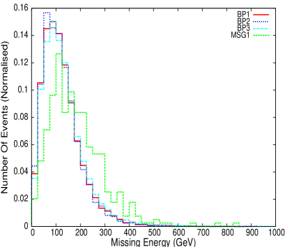
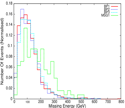
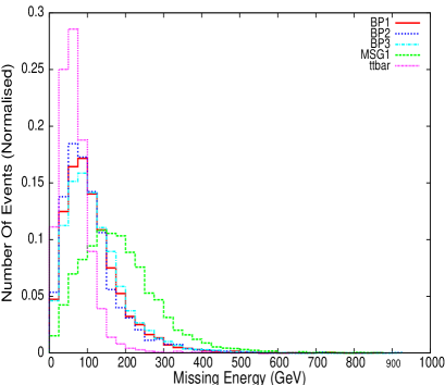
Figure 1: Missing energy distribution in $4b$, $4bl$ and $2b2l$ events from left to right and top to bottom before putting cut. CTEQ5L pdfset was used. Factorization and Renormalization scale has been set to $\mu_{F}=\mu_{R}=\sqrt{\hat{s}}$, sub-process centre of mass energy.

      

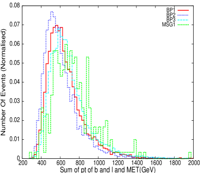
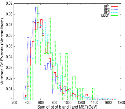
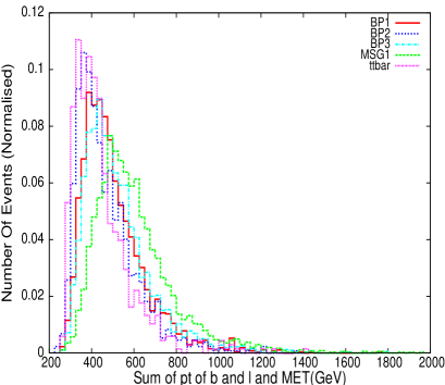
Figure 2: ‘$\Sigma p_{T}$ of $b$s and leptons and missing energy’ distribution in $4b$, $4bl$ and $2b2l$ events from left to right and top to bottom before putting cut. CTEQ5L pdfset was used. Factorization and Renormalization scale has been set to $\mu_{F}=\mu_{R}=\sqrt{\hat{s}}$, sub-process centre of mass energy.

4 Summary and Conclusions

In this work, we have proposed a scenario in which discovery of supersymmetry may be possible at the early runs of the LHC. Our scenario includes a light gluino and light 3rd family squarks, whereas the squarks for the first two families are very heavy. We work within the gravity mediated SUSY breaking scenario, but go beyond mSUGRA using non-universal boundary conditions for the gaugino masses, as well as for the sfermion masses.The gluinos are light enough to be pair produced copiously at the LHC. Their decays to sbottom-botom and stop-top gives rise to bottom quark rich final states with or without charged leptons together with large missing energy associated with the lightest (LSP) neutralino. The most promising final states are $4b+{E_{T}}\!\!\!\!/$, $4b+\ell+{E_{T}}\!\!\!\!/$ and $2b+2\ell+{E_{T}}\!\!\!\!/$. We have chosen three benchmark points and also one mSUGRA point with light gluino mass for comparison. With the cuts appropriate for the LHC, we find that the signal cross section for the $4b+{E_{T}}\!\!\!\!/$ channel is well above $1,000$ fb, whereas for the other two channels, it is well above $100$ fb. For comparison, the signal for the mSUGRA point (MSG1) is much smaller. The dominant background with the used cuts are from $t\bar{t}$ production which is significant for the $2b+2\ell+{E_{T}}\!\!\!\!/$ channel, but negligible for the $4b+{E_{T}}\!\!\!\!/$, $4b+\ell+{E_{T}}\!\!\!\!/$ channels. Thus as the LHC accumulates data this year to few hundred $pb^{-1}$ (or $1fb^{-1}$), the prospect of discovering SUSY in our proposed scenario is excellent., and we urge the ATLAS and CMS Collaborations to search for SUSY in these final states.

NOTE ADDED: During the completion of writing of this manuscript an article [29] in similar direction appeared in the arXiV. These authors also emphasize similar final states as in our work. They do not specify any SUSY breaking model, but rather use three different branching ratio for the gluino decays to choose their benchmark points. In our work, we use gravity mediated SUSY breaking framework, and generate the SUSY spectra from the high scale with non-universal boundary conditions, and satisfy the experimental constraints on the SUSY particle masses , dark matter and other low energy processes. Our results for the cross sections for the final states are in good agreement with their results.

Acknowledgment: SB would like to thank SN for his invitation to visit OSU and for the hospitality provided during the stay, when this work was formulated and carried out to a large extent. SB also acknowledges the support from Dr. Khanov at OSU for providing computer and cluster access which was used to a large extent for the computational part of this work.

References

- [1] For reviews on Supersymmetry, see, e.g., H. P. Nilles, Phys. Rep. 1, 110 ( 1984); H. E. Haber and G. Kane, Phys. Rep. 117, 75 ( 1985) ; J. Wess and J. Bagger, Supersymmetry and Supergravity, 2nd ed., (Princeton, 1991); H. Baer and X. Tata, Weak Scale Supersymmetry, Cambridge University Press, 2006; M. Drees, R. Godbole and P. Roy, Hackensack, USA: World Scientific (2004) 555 p; P. Binetruy, Oxford, UK: Oxford Univ. Pr. (2006) 520 p.
- [2] D. J. H. Chung et al., Phys. Rept. 407, 1 (2005); S. P. Martin, arXiv:hep-ph/9709356.
- [3] A. H. Chamseddine, R. Arnowitt and P. Nath, Phys. Rev. Lett. 49, 970 (1982); R. Barbieri, S. Ferrara and C. A. Savoy, Phys. Lett. B 119, 343 (1982); L. J. Hall, J. Lykken and S. Weinberg, Phys. Rev. D 27, 2359 (1983); P. Nath, R. Arnowitt and A. H. Chamseddine, Nucl. Phys. B 227, 121 (1983); N. Ohta, Prog. Theor. Phys. 70, 542 (1983).
- [4] U. Chattopadhyay and D. Das, Phys. Rev. D 79, 035007 (2009) [arXiv:0809.4065 [hep-ph]]; S. Bhattacharya, U. Chattopadhyay, D. Choudhury, D. Das and B. Mukhopadhyaya, Phys. Rev. D 81, 075009 (2010) [arXiv:0907.3428 [hep-ph]].
- [5] V. Berezinsky, A. Bottino, J. Ellis, N. Forrengo, G. Mignola, and S. Scopel, Astropart. Phys.5:1-26(1996).
- [6] P. Nath and R. Arnowitt, Phys. Rev. D 56, 2820 (1997); D. Feldman, Z. Liu and P. Nath, JHEP 0804, 054 (2008); D. Feldman, Z. Liu and P. Nath, Phys. Rev. D 78, 083523 (2008).
- [7] D. G. Cerdeno and C. Munoz, JHEP 0410, 015 (2004) [arXiv:hep-ph/0405057].
- [8] J. Ellis, K. A. Olive and P. Sandick, arXiv:0805.2343 [hep-ph]; J. R. Ellis, K. A. Olive, Y. Santoso and V. C. Spanos, Phys. Lett. B 603, 51 (2004); J. R. Ellis, T. Falk, K. A. Olive and Y. Santoso, Nucl. Phys. B 652, 259 (2003) [arXiv:hep-ph/0210205]; A. De Roeck et al., Y , J. R. Ellis, F. Gianotti, F. Moortgat, K. A. Olive and L. Pape, Eur. Phys. J. C 49, 1041 (2007) [arXiv:hep-ph/0508198].
- [9] H. Baer, A. Mustafayev, E. K. Park and X. Tata, JHEP 0805, 058 (2008); H. Baer et al., JHEP 0604, 041 (2006).
- [10] Y. Kawamura, H. Murayama and M. Yamaguchi, Phys. Rev. D 51 (1995) 1337 [arXiv:hep-ph/9406245]; Y. Kawamura, H. Murayama and M. Yamaguchi, Phys. Lett. B 324 (1994) 52 [arXiv:hep-ph/9402254].
- [11] A. Datta, A. Datta, M. Drees and D. P. Roy, Phys. Rev. D 61, 055003 (2000) [arXiv:hep-ph/9907444]; A. Datta, A. Datta and M. K. Parida, Phys. Lett. B 431, 347 (1998) [arXiv:hep-ph/9801242].
- [12] S. Bhattacharya, A. Datta and B. Mukhopadhyaya, Phys. Rev. D 78, 035011 (2008) [arXiv:0804.4051 [hep-ph]]; B. S. Acharya, P. Grajek, G. L. Kane, E. Kuflik, K. Suruliz and L. T. Wang, arXiv:0901.3367 [hep-ph].
- [13] J. R. Ellis, C. Kounnas and D. V. Nanopoulos, Nucl. Phys. B 247, 373 (1984); J. R. Ellis, K. Enqvist, D. V. Nanopoulos and K. Tamvakis, Phys. Lett. B 155, 381 (1985); M. Drees, Phys. Lett. B 158, 409 (1985); A. Corsetti and P. Nath, Phys. Rev. D 64, 125010 (2001) [arXiv:hep-ph/0003186]; A. Corsetti and P. Nath, Phys. Rev. D 64, 125010 (2001); U. Chattopadhyay, A. Corsetti and P. Nath, Phys. Rev. D 66, 035003 (2002); N. Chamoun, C. S. Huang, C. Liu and X. H. Wu, Nucl. Phys. B 624, 81 (2002) [arXiv:hep-ph/0110332]; U. Chattopadhyay and D. P. Roy, Phys. Rev. D 68, 033010 (2003); U. Chattopadhyay, D. Choudhury and D. Das, Phys. Rev. D 72, 095015 (2005); R. C. Cotta, J. S. Gainer, J. L. Hewett and T. G. Rizzo, Nucl. Phys. Proc. Suppl. 194, 133 (2009) [arXiv:0909.4088 [hep-ph]]; J. Chakrabortty and A. Raychaudhuri, Phys. Lett. B 673 (2009) 57 [arXiv:0812.2783 [hep-ph]].
- [14] S. Bhattacharya, A. Datta and B. Mukhopadhyaya, JHEP 0710, 080 (2007) [arXiv:0708.2427 [hep-ph]]; S. Bhattacharya, A. Datta and B. Mukhopadhyaya, Phys. Rev. D 78, 115018 (2008) [arXiv:0809.2012 [hep-ph]]; S. P. Martin, Phys. Rev. D 79, 095019 (2009) [arXiv:0903.3568 [hep-ph]]; S. Bhattacharya and J. Chakrabortty, Phys. Rev. D 81, 015007 (2010) [arXiv:0903.4196 [hep-ph]].
- [15] See for example, P. Konar, K. Kong and K. T. Matchev, JHEP 0903, 085 (2009) [arXiv:0812.1042 [hep-ph]]; M. M. Nojiri, K. Sakurai and B. R. Webber, JHEP 1006, 069 (2010) [arXiv:1005.2532 [hep-ph]].
- [16] See for example, N. Arkani-Hamed, G. L. Kane, J. Thaler and L. T. Wang, JHEP 0608, 070 (2006) [arXiv:hep-ph/0512190]; B. Bhattacherjee, A. Kundu, S. K. Rai and S. Raychaudhuri, Phys. Rev. D 81, 035021 (2010) [arXiv:0910.4082 [hep-ph]]; K. Ghosh, S. Mukhopadhyay and B. Mukhopadhyaya, JHEP 1010, 096 (2010) [arXiv:1007.4012 [hep-ph]].
- [17] V. D. Barger, C. Kao and R. J. Zhang, Phys. Lett. B 483 (2000) 184 [arXiv:hep-ph/9911510].
- [18] Y. Nir and N. Seiberg, Phys. Lett. B 309 (1993) 337 [arXiv:hep-ph/9304307]; M. Dine, A. E. Nelson and Y. Shirman, Phys. Rev. D 51 (1995) 1362 [arXiv:hep-ph/9408384]; L. Randall and R. Sundrum, Nucl. Phys. B 557 (1999) 79 [arXiv:hep-th/9810155].
- [19] S. Chen, et al., CLEO Collaboration, Phys. Rev. Lett. 87, 251807 (2001), hep-ex/0108032; P. Koppenburg et al. [Belle Collaboration], Phys. Rev. Lett. 93, 061803 (2004) B. Aubert, et al., BaBar Collaboration, hep-ex/0207076.
- [20] E. Komatsu et al. [WMAP Collaboration], arXiv:0803.0547 [astro-ph].
- [21] A. Djouadi, J. L. Kneur and G. Moultaka, arXiv:hep-ph/0211331.
- [22] G. Belanger, F. Boudjema, A. Pukhov and A. Semenov, Comput. Phys. Commun. 176, 367 (2007) [arXiv:hep-ph/0607059].
- [23] T. Sjostrand, S. Mrenna and P. Skands, JHEP 0605, 026 (2006) [arXiv:hep-ph/0603175].
- [24] P. Skands et al., JHEP 0407, 036 (2004) [arXiv:hep-ph/0311123].
- [25] H. L. Lai et al. [CTEQ Collaboration], Eur. Phys. J. C 12, 375 (2000) [arXiv:hep-ph/9903282].
- [26] ATLAS detector and physics performance. Technical design report. Vol. 2, CERN-LHCC-99-15, ATLAS-TDR-15.
- [27] Private communication with Dr. Bruce Melado; S. Biswas and B. Mukhopadhyaya, Phys. Rev. D 81, 015003 (2010) [arXiv:0910.3446 [hep-ph]].
- [28] N. Desai and B. Mukhopadhyaya, Phys. Rev. D 80, 055019 (2009) [arXiv:0901.4883 [hep-ph]]; H. Baer, V. Barger, A. Lessa and X. Tata, JHEP 1006, 102 (2010) [arXiv:1004.3594 [hep-ph]]; M. A. Ajaib, T. Li, Q. Shafi and K. Wang, arXiv:1011.5518 [hep-ph]; S. Bornhauser, M. Drees, S. Grab and J. S. Kim, arXiv:1011.5508 [hep-ph]; N. Chen, D. Feldman, Z. Liu, P. Nath and G. Peim, arXiv:1011.1246 [hep-ph]; N. Chen, D. Feldman, Z. Liu, P. Nath and G. Peim, arXiv:1010.0939 [hep-ph].
- [29] G. L. Kane, E. Kuflik, R. Lu and L. T. Wang, arXiv:1101.1963 [hep-ph].