Particle identification

Abstract

Particle IDentification (PID) is fundamental to particle physics experiments. This paper reviews PID strategies and methods used by the large LHC experiments, which provide outstanding examples of the state-of-the-art. The first part focuses on the general design of these experiments with respect to PID and the technologies used. Three PID techniques are discussed in more detail: ionization measurements, time-of-flight measurements and Cherenkov imaging. Four examples of the implementation of these techniques at the LHC are given, together with selections of relevant examples from other experiments and short overviews on new developments. Finally, the Alpha Magnetic Spectrometer (AMS 02) experiment is briefly described as an impressive example of a space-based experiment using a number of familiar PID techniques.

1 Introduction

In addition to tracking and calorimetry, Particle IDentification (PID) is a crucial aspect of most particle physics experiments. The identification of stable particles is achieved either by analysing the way they interact, or by determining their mass. The difference in interaction is primarily used for lepton and photon identification. A “traditional” particle physics experiment already incorporates this method in its conceptual design, as it is discussed in Sect. 1.1. In order to unambiguously identify hadrons, their charge and mass has to be determinded, which is achieved by simultaneous measurements of momentum and velocity. This method is discussed in Sect. 1.2.

The four large experiments at the CERN Large Hadron Collider (LHC) [1] and their PID strategies are introduced briefly in Sect. 2. Three methods to determine the mass of a charged particle and examples of their implementation at the LHC experiments are discussed in Sects. 3 (ionization), 4 (time-of-flight) and 5 (Cherenkov radiation imaging). A fourth important method, the detection of transition radiation, is not discussed, since it is the topic of a separate paper in this issue [2]. In Sect. 6 finally the AMS 02 experiment is briefly described as an example for the usage of PID techniques from accelerator-based particle physics experiments in space.

1.1 PID by difference in interaction

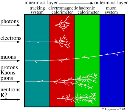
Figure 1: Components of a “traditional” particle physics experiment. Each particle type has its own signature in the detector. For example, if a particle is detected only in the electromagnetic calorimeter, it is fairly certain that it is a photon.

In a “traditional” particle physics experiment particles are identified (electrons and muons, their antiparticles and photons), or at least assigned to families (charged or neutral hadrons), by the characteristic signatures they leave in the detector. The experiment is divided into a few main components, as shown in Fig. 1, where each component tests for a specific set of particle properties. These components are stacked in layers and the particles go through the layers sequentially from the collision point outwards: first a tracking system, then an electromagnetic (EM) and a hadronic calorimeter and a muon system. All layers are embedded in a magnetic field in order to bend the tracks of charged particles for momentum and charge sign determination.

1.1.1 Tracking system

The tracking system determines whether the particles are charged. In conjunction with a magnetic field, it measures the sign of the charge and the momentum of the particle. Photons may convert into an electron-positron pair and can in that case be detected in the tracking system. Moreover, charged kaon decays may be detected in a high-resolution tracking system through their characteristic “kink” topology: e.g. K${}^{\pm}\rightarrow\mu^{\pm}\nu_{\mu}$ (64%) and K${}^{\pm}\rightarrow\pi^{\pm}\pi^{0}$ (21%). The charged parent (kaon) decays into a neutral daughter (not detected) and a charged daughter with the same sign. Therefore, the kaon identification process reduces to the finding of kinks in the tracking system. The kinematics of this kink topology allows to separate kaon decays from the main source of background kinks coming from charged pion decays [3].

1.1.2 Calorimeters

Calorimeters detect neutral particles, measure the energy of particles, and determine whether they have electromagnetic or hadronic interactions. EM and hadron calorimetry at the LHC is described in detail in Refs. [4, 5]. PID in a calorimeter is a destructive measurement. All particles except muons and neutrinos deposit all their energy in the calorimeter system by production of electromagnetic or hadronic showers. The relative resolution with which the deposited energy is measured is usually parametrised as:

$$\left(\frac{\sigma_{E}}{E}\right)^{2}=\left(\frac{a}{\sqrt{E}}\right)^{2}+\left(\frac{b}{E}\right)^{2}+c^{2}\ .$$ (1)

The first term takes into account the stochastic fluctuations and limits the low energy performance. The second term is due to electronics noise. The third, constant term takes into account detector uniformities and errors in the calibration. This term limits the calorimeter performance at high energies. Fig. 2 shows a comparison of the relative resolutions for the EM and hadronic calorimeters of the different LHC experiments.

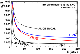
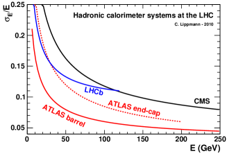
Figure 2: Comparison of the relative energy resolutions (as given by Eq. 1) of the different EM calorimeters (left image) and hadronic calorimeters (right image) at the LHC experiments. The values of the parameters $a$, $b$ and $c$ were in all cases determined by fits to the data from beam tests and are given in the descriptions of the different experiments in Sects. 2.1, 2.2 and 2.3. In case of the ATLAS and CMS hadronic calorimeters the resolutions of the whole systems combining EM and hadronic calorimeters are shown.

Calorimeters may be broadly classified into one of two types: sampling calorimeters and homogeneous calorimeters. Sampling calorimeters consist of layers of a dense passive absorber material interleaved with active detector layers. In homogeneous calorimeters on the other hand the absorber also acts as the detection medium.

Photons, electrons and positrons deposit all their energy in the EM calorimeter. Their showers are indistinguishable, but an electron can be identified by the existence of a track in the tracking system that is associated to the shower. In this case the energy deposit must match the momentum measured in the tracking system. Hadrons on the other hand deposit most of their energy in the hadronic calorimeter (part of it is also deposited in the EM calorimeter). However, the individual members of the families of charged and neutral hadrons can not be distinguished in a calorimeter.

1.1.3 Muon system

Muon systems at the LHC are described in detail in Ref. [6]. The muon differs from the electron only by its mass, which is around a factor 200 larger. As a consequence, the critical energy $E_{c}$ (the energy for which in a given material the rates of energy loss through ionization and bremsstrahlung are equal) is much larger for muons: it is around 400 GeV for muons on copper, while for electrons on copper it is only around 20 MeV. As a consequence, muons do in general not produce electromagnetic showers and can thus be identified easily by their presence in the outermost detectors, as all other charged particles are absorbed in the calorimeter system.

1.1.4 Other particles

Neutrinos do in general not interact in a particle detector of the sort shown in Fig. 1, and therefore escape undetected. However, their presence can often be inferred by the momentum imbalance of the visible particles. In electron-positron colliders it is usually possible to reconstruct the neutrino momentum in all three dimensions and its energy.

Quark flavor tagging identifies the flavor of the quark that is the origin of a jet. The most important example is B-tagging, the identification of beauty quarks. Hadrons containing beauty quarks can be identified because they have sufficient lifetime to travel a small distance before decaying. The observation of a secondary vertex a small distance away from the collision point indicates their presence. For this the information of a high-precision tracking system around the collision point is used. Such vertex tracking detectors are described in detail in Ref. [7]. Also Tau leptons, with a mean lifetime of 0.29 ps, fly a small distance (about 0.5 mm) before decaying. Again, this is typically seen as a secondary vertex, but without the observation of a jet.

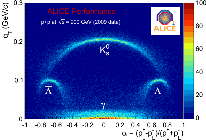
Figure 3: Armenteros-Podolanski plot from the ALICE experiment using data from $\sqrt{s}=900$ GeV proton collisions. The different V₀ particles can be separated using the kinematics of their decay products. The orientation of the decay is described with respect to the momentum vector of the $V_{0}$. $p^{\pm}_{L}$ are the longitudinal momenta of the positively and negatively charged decay products with respect to the V₀ particle’s direction. $q_{T}$ represents the transverse component of the momentum of the positive decay product.

K${}_{S}^{0}$, $\Lambda$ and $\bar{\Lambda}$ particles are collectively known as V⁰ particles, due to their characteristic decay vertex, where an unobserved neutral strange particle decays into two observed charged daughter particles: e.g. K${}_{S}^{0}\rightarrow\pi^{+}\,\pi^{-}$ and $\Lambda\rightarrow$p $\pi^{-}$. V⁰ particles can be identified from the kinematics of their positively and negatively charged decay products (see Fig.3) [8].

1.2 PID by mass determination

The three most important charged hadrons (pions, kaons and protons) and their antiparticles have identical interactions in an experimental setup as the one shown in Fig. 1 (charge deposit in the tracking system and hadronic shower in the calorimeter). Moreover, they are all effectively stable. However, their identification can be crucial, in particular for the study of hadronic decays. The possible improvement in the signal-to-background ratio when using PID is demonstrated in Fig. 4, using the example of the $\phi\rightarrow$ K⁺K^- decay.

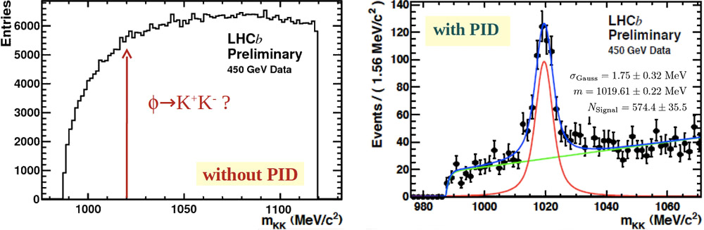
Figure 4: Demonstration of the power of PID by mass determination, using the example of the $\phi\rightarrow$ K⁺K^- decay measured with the LHCb RICH system (preliminary data from $\sqrt{s}=900$ GeV p–p collisions [9]). The left image shows the invariant mass obtained from all combinations of pairs of tracks without PID. The right image shows how the $\phi$ meson signal appears when tracks can be identified as kaons.

In B physics, the study of hadrons containing the beauty quark, different decay modes usually exist, and their individual properties can only be studied with an efficient hadron identification, which improves the signal-to-background ratio (most tracks are pions from many sources).

PID is equally important in heavy-ion physics. An example is the measurement of open charm (and open beauty), which allows to investigate the mechanisms for the production, propagation and hadronization of heavy quarks in the hot and dense medium produced in the collision of heavy ions. The most promising channel is D${}^{0}\rightarrow\mbox{K}^{-}\pi^{+}$. It requires a very efficient PID, due to the small signal-to-background ratio.

In order to identify any stable charged particle, including charged hadrons, it is necessary to determine its charge $ze$ and its mass $m$. The charge sign is obtained from the curvature of the particle’s track. Since the mass can not be measured directly, it has to be deduced from other variables. These are in general the momentum $p$ and the velocity $\beta=v/c$, where one exploits the basic relationship

$$p=\gamma mv\quad\rightarrow\quad m=\frac{p}{c\beta\gamma}\ .$$ (2)

Here $c$ is the speed of light in vacuum and $\gamma=(1-\beta^{2})^{-1/2}$ is the relativistic Lorentz factor. The resolution in the mass determination is

$$\left(\frac{\mbox{d}m}{m}\right)^{2}=\left(\frac{\mbox{d}p}{p}\right)^{2}+\left(\gamma^{2}\frac{\mbox{d}\beta}{\beta}\right)^{2}.$$ (3)

Since in most cases $\gamma\gg 1$, the mass resolution is determined mainly by the accuracy of the velocity measurement, rather than the momentum determination.

The momentum is obtained by measuring the curvature of the track in the magnetic field. The particle velocity is obtained by means of one of the following methods:

1. measurement of the energy deposit by ionization,

2. time-of-flight (TOF) measurements,

3. detection of Cherenkov radiation or

4. detection of transition radiation.

Each of these methods provide PID not only for charged hadrons, but also for charged leptons. The small obstacle of muons and pions not being well separated due to $m_{\mu}\approx m_{\pi}$ can luckily be circumnavigated, since muons can be easily identified by other means.

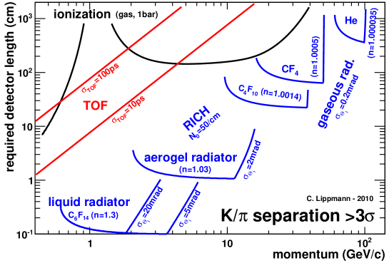
Figure 5: Approximate minimum detector length required to achieve a K/$\pi$ separation of $n_{\sigma}\geq 3\,\sigma$ with three different PID techniques. For the energy loss technique we assume a gaseous detector. For the TOF technique, the detector length represents the particle flight path over which the time-of-flight is measured. For the Cherenkov technique only the radiator thickness is given. The thicknesses of an expansion gap and of the readout chambers have to be added.

The use of these methods is restricted to certain momentum ranges. For a given momentum range, the separation power can be used to quantify the usability of a technique. It defines the significance of the detector response $R$. If $R_{A}$ and $R_{B}$ are the mean values of such a quantity measured for particles of type $A$ and $B$, respectively, and $\langle\sigma_{A,B}\rangle$ is the average of the standard deviations of the measured distributions, then the separation power $n_{\sigma}$ is given by

$$n_{\sigma}=\frac{R_{A}-R_{B}}{\langle\sigma_{A,B}\rangle}\ .$$ (4)

A summary of the momentum coverage and required detector lengths using the example of K/$\pi$ separation with the requirement $n_{\sigma}\geq 3$ is given in Fig. 5.

Naturally, when choosing a PID technique, also other features have to be considered besides the separation power. In practice, these often include luminosity and event rates, size and space requirements, accessibility, multiple scattering in the used materials, compatibility with other detector subsystems and geometrical coverage.

2 Overview of the large LHC experiments

The four main LHC experiments are the largest current collider experiments and integrate todays state-of-the-art detector technology, in particular with respect to PID. This section gives an overview on the four experiments, with emphasis on the way the underlying physics program influences the experiment design with respect to PID.

2.1 ATLAS and CMS

ATLAS [10] (A Toroidal Large AparatuS) and CMS [11] (Compact Muon Solenoid) are often called “general purpose” particle physics experiments, since they aim at uncovering any new phenomena appearing in proton–proton (p–p) collisions at the new energy domain that is now probed at the LHC. The main focus of the experiments is the investigation of the nature of the electroweak symmetry breaking and the search for the Higgs boson. The experimental study of the Higgs mechanism is expected to shed light on the mathematical consistency of the Standard Model (SM) of particle physics at energy scales above $\sim$1 TeV. As a matter of fact, various alternatives to the SM foresee new symmetries, new forces, and new constituents. Furthermore, there are high hopes for discoveries that could lead towards a unified theory (supersymmetry, extra dimensions, …).

2.1.1 Requirements

The discovery and study of the Higgs boson is the benchmark process that influenced the design of the two experiments. Electrons, muons and photons are important components of its possible physics signatures. Assuming a low mass Higgs boson ($m_{H}<150$ GeV/c²), the predominant decay mode into hadrons is difficult to detect due to QCD backgrounds. In that case an important decay channel is $H\rightarrow\gamma\gamma$. For masses above 130 GeV, the most promising channel to study the properties of the Higgs boson is $H\rightarrow ZZ^{(*)}\rightarrow 4\,l$. It is called “gold-plated” in the particular case in which all four leptons are muons, due to the relative ease in detecting muons. The ATLAS and CMS detectors have been optimised to cover the whole spectrum of possible Higgs particle signatures. In summary, these are the requirements:

1. large acceptance in pseudo-rapidity and almost full coverage in azimuthal angle (the angle around the beam direction);

2. good identification capabilities for isolated high transverse momentum photons and electrons;

3. good muon ID and momentum resolution over a wide range of momenta and angles. At highest momenta (1 TeV) a transverse momentum resolution $\sigma_{p_{T}}/p_{T}$ of the order 10% is required.

To maximize the integrated luminosity for the rare processes that are the main interest of the experiments, proton bunches will be brought to collision every 25 ns. Strong focusing of the beams helps to increase the luminosity to $10^{34}$ cm^-2s^-1. The consequences are a large number of overlapping events per proton bunch crossing and extreme particle rates. For the experiments these pose major challenges.

2.1.2 Setup

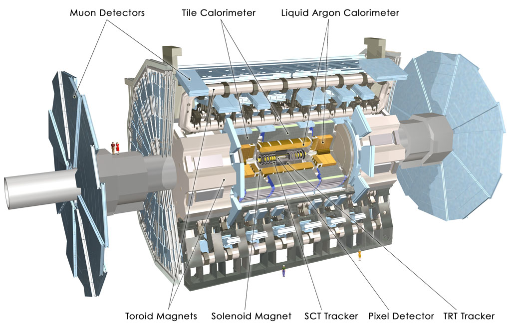
Figure 6: Perspective view of the ATLAS detector [10]. The dimensions are 25 m in height and 44 m in length, the overall weight of the detector is approximately 7000 tonnes.

The setup of ATLAS and CMS is in general quite similar, following the “traditional” setup as described in Sect. 1.1. However, in the implementation of some of the components quite different choices were made. The main similarities and some differences can be seen in Tab. 1. Schematic images of the two detectors are shown in Figs. 6 and 7.

Table 1: Overview on the technologies chosen for the ATLAS and CMS tracking systems, EM and hadronic calorimeters and muon systems. Their acceptances in pseudo-rapidity $\eta$ are given as well. Abbreviations are explained in the text.

Detector	technology		$\eta$-coverage
component	ATLAS	CMS	ATLAS	CMS
Tracking	Si pixel detector (3 layers)
	Si strip detector		$|\eta|<2.5$
	SCT (4 layers)	(10 layers)
	TRT (straw tubes)	-
EM Cal	Sampling	Homogeneous	$|\eta|<3.2$	$|\eta|<3.0$
	(Pb / LAr)	(PbWO4 crystals)
H Cal	Sampling	Sampling
	(Barrel: Iron / Scint.	(Brass / Scint.)	$|\eta|<3.2$	$|\eta|<3.0$
	End-caps: Cu / LAr)
Muon	CSC (inner plane)	CSC	$2<|\eta|<2.7$	$0.9<|\eta|<2.4$
(Tracking)	MDT	DT	$|\eta|<2.7$ ($2.0$	$|\eta|<1.2$
			for inner plane)
Muon	Bakelite RPC		$|\eta|<1.05$	$|\eta|<1.6$
(Trigger)	TGC	-	$1.05<|\eta|<2.7$	-

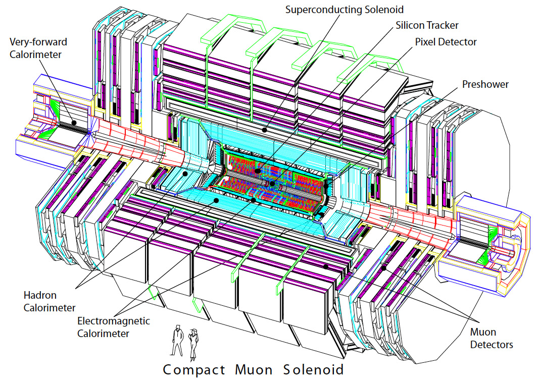
Figure 7: Perspective view of the CMS detector [11]. The dimensions are 14.6 m in height and 21.6 m in length. The overall weight is approximately 12 500 tonnes.

2.1.3 Tracking and muon systems

As the innermost component, the tracking systems of ATLAS and CMS are embedded in solenoidal magnetic fields of 2 T and 4 T, respectively. In both cases the tracking systems consist of silicon pixel and strip detectors. ATLAS includes also a Transition Radiation Tracker (TRT) based on straw tubes, which provides also electron ID [2].

The global detector dimensions are defined by the large muon spectrometers, which are designed to measure muon momenta with extremely high accuracy [6]. While the muon system of ATLAS is designed to work independently of the inner detector, in CMS the information from the tracking system is in general combined with that from the muon system.

The ATLAS muon system uses eight instrumented air-core toroid coils, providing a magnetic field mostly orthogonal to the muon trajectories, while minimising the degradation of resolution due to multiple scattering [10]. For high-precision tracking, the magnets are instrumented with Monitored Drift Tubes (MDT) and, at large pseudo-rapidities, Cathode Strip Chambers (CSC). By measuring muon tracks with a resolution $\leq$50 $\mu$m, a standalone transverse momentum resolution $\sigma(p_{T})/p_{T}\approx 3$% is achieved for $p_{T}=100$ GeV/c, while at $p_{T}=1$ TeV/c it is around 10%. Only below 200 GeV/c the combination of the information from the muon and tracking systems helps, keeping the resolution below 4%. As a separate trigger system and for second coordinate measurement, Resistive Plate Chambers (RPCs) are installed in the barrel, while Thin Gap Chambers (TGCs) are placed in the end-caps, where particle rates are higher.

The CMS design relies on the high bending power (12 Tm) and momentum resolution of the tracking system, and uses an iron yoke to increase its magnetic field [11]. With the field parallel to the LHC beam axis, the muon tracks are bent in the transverse plane. The iron yoke is instrumented with aluminum Drift Tubes (DT) in the barrel and CSCs in the end-cap region. Due to the iron yoke, the momentum resolution of the CMS muon system is dominated by the multiple scattering. As a consequence, the requirements on spatial resolution are somewhat looser ($\sim$70 $\mu$m) than in ATLAS. The standalone muon momentum resolution is $\sigma(p_{T})/p_{T}=9$% for $p_{T}\leq 200$ GeV/c and 15 to 40% at $p_{T}=1$ TeV/c, depending on $|\eta|$. Including the tracking system improves the result by an order of magnitude for low momenta. At 1 TeV the contribution of both measurements together yield a momentum resolution of about 5%. The DT and CSC subsystems can each trigger on muons with large transverse momentum. However, for the full LHC luminosity, faster trigger chambers are needed to associate the detected muons to the right crossing of proton bunches in the LHC. RPCs are used throughout the whole CMS muon system for that purpose.

2.1.4 Particle identification

Electrons, hadrons and neutral particles are identified in the calorimeter systems, while muons are identified in the large muon systems. The designs of the EM calorimeters and muon systems have been guided by the benchmark processes of Higgs boson decays into two photons or into leptons.

The ATLAS EM calorimeter is of sampling type and consists of liquid Argon (LAr) as detection medium and lead (Pb) absorber plates operated in a cryostat at 87 K. The calorimeter depth varies from 22 to 38 $X_{0}$, depending on the pseudo-rapidity range. In beam tests [10] the relative energy resolution after subtraction of the noise term was found to be $(\sigma_{E}/E)^{2}=(0.1/\sqrt{E\,(\mbox{GeV})})^{2}+0.007^{2}$. The CMS EM calorimeter on the other hand is a homogeneous calorimeter made from lead tungstate (PbWO₄) crystals with a length that corresponds to around $25\,X_{0}$. The relative energy resolution was measured in beam tests as $(\sigma_{E}/E)^{2}=(0.028/\sqrt{E\,(\mbox{GeV})})^{2}+(0.125/E($ GeV$))^{2}+0.003^{2}$.

The ATLAS hadronic calorimeter is made from a Barrel and two end-cap modules. The barrel part is made from steel and plastic scintillator tiles. The end-caps are made from copper plates and use LAr as active medium. In beam tests of the combined EM and hadronic calorimeter systems the relative energy resolution [10] for pions was found to be $(\sigma_{E}/E)^{2}=(0.52/\sqrt{E\,(\mbox{GeV})})^{2}+(0.016/E($ GeV$))^{2}+0.03^{2}$ in the barrel and $(\sigma_{E}/E)^{2}\approx(0.84/\sqrt{E\,(\mbox{GeV})})^{2}$ in the end-caps. The CMS hadronic calorimeter is made from brass and plastic scintillator tiles. The resulting energy resolution [12] for the combined system of EM and hadronic calorimeters and for pions is $(\sigma_{E}/E)^{2}=(1.12/\sqrt{E\,(\mbox{GeV})})^{2}+0.036^{2}$.

The silicon detectors of the ATLAS and CMS tracking systems offer the possibility of hadron ID at low momenta (a few hundred MeV/c) via ionization measurements. For electron ID at momenta up to 25 GeV/c ATLAS also takes into account the information from the TRT, namely large energy deposits by electrons due to transition radiation (for details see Ref. [2]).

2.2 ALICE

ALICE [13] (A Large Ion Collider Experiment) is the dedicated heavy-ion experiment at the LHC. The LHC can collide lead (Pb) nuclei at center-of mass energies of $\sqrt{s_{NN}}=2.76$ and 5.5 TeV. This leap to up to 28 times beyond what is presently accessible will open up a new regime in the experimental study of nuclear matter. The aim of ALICE is to study the physics of strongly interacting matter at the resulting extreme energy densities and to study the possible formation of a quark-gluon plasma. Many observables meant to shed light on the evolution of the quark-gluon plasma depend on PID. The most natural example is particle spectra, from which the freeze-out parameters (such as the kinetic and chemical freeze-out temperature and the collective flow velocity) can be extracted. Besides pions, kaons and protons, also resonances such as the $\phi$ meson can be used for such analysis. Actually, any modification in the mass and width of the $\phi$ meson could be a signature for partial chiral symmetry restoration, and thus, creation of a quark-gluon plasma. The $\phi$ resonance is typically identified via its hadronic decay channel $\phi\rightarrow K^{+}K^{-}$, which makes a good hadron ID important. Leptonic channels are very important as well and thus extremely good lepton ID is needed.

ALICE also studies p–p collisions at $\sqrt{s}=7$ and 14 TeV. These data are important as a reference for the heavy-ion data. Moreover, due to the very low momentum cut-off ($\sim$0.1 GeV/c), ALICE can contribute in physics areas where it complements the other LHC experiments. To name an example, the measurement of charm and beauty cross sections is possible down to very low momenta. Moreover, proton physics at high multiplicities is easily accessible via the multiplicity trigger from the Silicon Pixel Detector (SPD).

2.2.1 Requirements

As compared to p–p collisions, the charged track multiplicities in Pb–Pb collisions are extraordinary. At the time of the ALICE Technical Proposal, charged particle densities of up to d$N_{\text{ch}}$/d$\eta=8000$ were considered for the LHC center-of-mass energy [14, 15, 16] . Including secondaries, this would amount to 20 000 tracks in one interaction in the relevant acceptance region. However, first measurements [17] at $\sqrt{s_{NN}}=2.76$ TeV yield d$N_{\text{ch}}$/d$\eta\approx 1600$. When compared to p–p collisions at the LHC, the produced particles have relatively low momenta: i.e. 99% have a momentum below about 1 GeV/c. Hadrons, electrons, muons and photons may be used as probes in order to explore the strongly interacting matter that is produced in the Pb–Pb collisions. Those probes are inspected by dedicated PID detectors. In some cases these detectors may have very limited geometrical acceptance; for some actually not even a coverage of 2 $\pi$ in azimuthal angle is necessary. This is an important difference when compared to general purpose experiments. Nevertheless, large geometrical acceptance remains important for the main tracking devices. In summary, these are the requirements for the ALICE experiment:

1. reliable operation in an environment of very large charged track multiplicities;

2. precision tracking capabilities at very low momenta (100 MeV/c), but also up to 100 GeV/c;

3. low material budget;

4. low magnetic field ($0.2\leq B\leq 0.5$ T) in order to be able to track low momentum particles;

5. good hadron ID for momenta up to a few GeV/c and electron ID up to 10 GeV/c in the central barrel;

6. good muon ID (in the forward region).

At LHC energies the total cross-section for Pb–Pb collisions will be of the order of 8 b. At the maximum expected luminosity of $10^{27}$ cm^-2s^-1 this corresponds to an interaction rate of 8 kHz. Only a fraction of these events will be central collisions (collisions with small impact parameter) and the aim is to be able to trigger on at least 200 of such central events per second.

For p–p collisions the goal is to be able to read out the experiment at rates of at least 1.4 kHz. Since the specific features of the used detectors (TPC drift time of almost 100 $\mu$s, see Sect. 3.7) makes it a rather slow detector (at least compared to the three other large LHC experiments), the luminosity for p–p collisions has to be limited [15]: at $\sim$$5\times 10^{30}$ cm^-2s^-1, corresponding to an interaction rate of $\sim$200 kHz, the integrated luminosity can be maximised for rare processes. With lower luminosity ($10^{29}$ cm^-2s^-1) statistics for large cross section observables can be collected and global event properties can be studied at optimum detector performance.

2.2.2 Setup

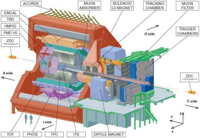
Figure 8: Perspective view of the ALICE detector [13]. The dimensions are 16 m in height and 26 m in length. The overall weight is approximately 10 000 tonnes.

The ALICE experimental setup is shown in Fig. 8. ALICE consists of a central barrel part for the measurement of hadrons, leptons and photons, and a forward muon spectrometer. The central part is embedded in a large solenoid magnet that is reused from the L3 experiment at the LEP collider at CERN.

A Time Projection Chamber (TPC) was chosen as the main tracking device in the central barrel, as this is a very high granularity detector capable of satisfying the requirements given in the previous section. The TPC surrounds the Inner Tracking System (ITS) which is optimised for the determination of primary and secondary vertices and for precision tracking of low-momentum particles. As the innermost layer, the Silicon Pixel Detector (SPD) has a key role in the determination of the vertex position. A unique feature of the SPD is its capability to generate a prompt trigger based on a programmable, fast online algorithm. As second and third layers, a Silicon Drift Detector (SDD) and a Silicon Strip Detector (SSD) complete the ITS, with two detection planes each. Finally, on the outside of the TPC, the Transition Radiation Detector (TRD) contributes to the tracking capability and provides electron ID [2].

2.2.3 Particle identification

The strategy for PID in the barrel of ALICE is described in detail in Ref. [16]. In a first step, all charged particles from the collision are tracked in the ITS, TPC and TRD using parallel Kalman filtering. The PID procedure is then applied to all reconstructed tracks that have been successfully associated to a signal in one of the PID detectors.

The TPC, SSD and SDD each provide PID via ionization measurements. The TPC is described in more detail in Sect. 3.7. The TRD is designed for electron ID and is described in Ref. [2]. The time-of-flight (TOF) array provides charged hadron ID and is described in Sect. 4.5.

Surrounding the TOF detector, there are three single-arm detectors inside the ALICE solenoid magnet: the Photon Spectrometer (PHOS), the Electro-Magnetic CALorimeter (EMCAL) and an array of RICH counters optimised for High-Momentum Particle IDentification (HMPID, see Sect. 5.3). PHOS is a homogeneous EM calorimeter based on lead tungstate crystals, similar to the ones used by CMS, read out using Avalanche Photodiodes (APD). It covers 100 deg in azimuthal angle and $|\eta|\leq 0.12$ in pseudo-rapidity. Its thickness corresponds to 20 $X_{0}$. The crystals are kept at a temperature of 248 K to minimize the contribution of noise to the energy resolution, optimizing the response for low energies. In a beam test the relative energy resolution was found to be $(\sigma_{E}/E)^{2}=(0.033/\sqrt{E\,(\mbox{GeV})})^{2}+(0.018/E\,($GeV$))^{2}+0.011^{2}$. The EMCAL was proposed as a late addition to the ALICE setup, with the primary goal to improve the capabilities of ALICE for jet measurements. The main design criterion was to provide as much EM calorimetry coverage as possible within the constraints of the existing ALICE detector systems. The EMCAL is a sampling calorimeter made from lead absorber plates and scintillators and is positioned opposite in azimuth to the PHOS, covering 107 deg in azimuthal angle and $|\eta|\leq 0.7$ in pseudo-rapidity. The relative energy resolution of the EMCAL was measured in a test beam and can be parameterised as $(\sigma_{E}/E)^{2}=(0.113/\sqrt{E\,(\mbox{GeV})})^{2}+0.0168^{2}$.

The goal of the ALICE muon spectrometer is to study vector mesons containing heavy quarks, such as $J/\Psi$, $\Psi^{\prime}$ and members of the $\Upsilon$ family via the muonic channel. The muon spectrometer covers only the limited pseudo-rapidity interval $2.5\leq\eta\leq 4$. Closest to the interaction region there is a front absorber to remove hadrons and photons emerging from the collision. Five pairs of high-granularity detector planes form the tracking system within the field of a large dipole magnet. Beyond the magnet is a muon filter (a 120 cm thick iron wall), followed by two pairs of trigger chamber planes (RPCs).

2.3 LHCb

LHCb [18] is dedicated to heavy flavor physics. One particular aim is to look at evidence of new physics in CP violation and rare decays of beauty and charm hadrons. The level of CP violation in the SM can not explain the absence of antimatter in our universe. A new source of CP violation is needed to understand this matter-antimatter asymmetry, implying new physics. Particles associated with new physics could manifest themselves indirectly in beauty or charm meson decays and produce contributions that change the expectations of CP violation phases. They may also generate decay modes forbidden in the SM.

2.3.1 Requirements

A large $b\bar{b}$ production cross section of the order $\sim$500 $\mu$b is expected for p–p collisions at $\sqrt{s}=14$ TeV. At high energies, the $b\bar{b}$ pairs are predominantly produced in a forward or backward cone. Separating pions from kaons in selected B hadron decays is fundamental to the physics goals of LHCb. A good example is the channel $B_{S}^{0}\rightarrow D_{S}^{\mp}K^{\pm}$, which has to be separated from the background from $B_{S}^{0}\rightarrow D_{S}^{-}\pi^{+}$, which is about 15 times more abundant. Moreover, other final states containing electrons, muons and neutral particles (photons, neutral pions and $\eta$’s) have to be distinguishable. The requirements for the LHCb detector can be summarised in this way:

1. geometrical acceptance in one forward region ($1.9<\eta<4.9$);

2. good hadron ID;

3. good momentum and vertex resolutions and

4. an efficient and flexible trigger system.

In order to maximize the probability of a single interaction per beam crossing, the luminosity in the LHCb interaction region may be limited to 2 to $5\times 10^{32}$cm^-2s^-1. In these conditions, one year of LHCb running ($\sim$10⁷ s) corresponds to 2 fb^-1 of integrated luminosity and about $10^{12}$ $b\bar{b}$ pairs produced in the region covered by the spectrometer.

2.3.2 Setup

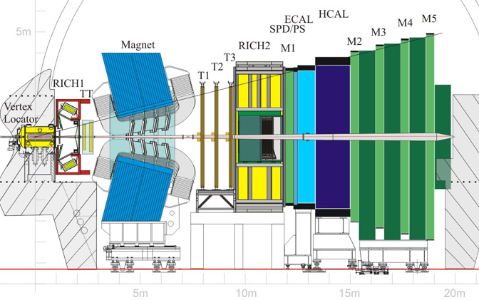
Figure 9: Schematic view of the LHCb detector [18].

Unlike ATLAS and CMS, LHCb does not have a cylindrical geometry. Rather, it is laid out horizontally along the beam line, as shown in Fig. 9. The tracking system consists of the VErtex LOcator (VELO) and four planar tracking stations: the Tracker Turicensis (TT) upstream of the 4 Tm dipole magnet, and stations T1-T3 downstream of the magnet. VELO and TT use silicon strip detectors. In T1-T3, silicon strips are used in the region close to the beam pipe, whereas strawtubes are employed in the outer regions. The VELO makes possible a reconstruction of primary vertices with 10 $\mu$m (60 $\mu$m) precision in the transverse (longitudinal) direction. In this way the displaced secondary vertices, which are a distinctive feature of beauty and charm hadron decays, may be identified. The overall performance of the tracking system enables the reconstruction of the invariant mass of beauty mesons with resolution $\sigma_{m}\approx 15$ to $20$ MeV/c², depending on the channel.

2.3.3 Particle identification

LHCb in general looks like a slice out of a “traditional” experiment as described in Sect. 1.1, apart from the two RICH detectors providing hadron ID. The RICH detectors are described in more detail in Sect. 5.4. An EM calorimeter and a hadron calorimeter provide the identification of electrons, hadrons and neutral particles (photons and $\pi_{0}$) as well as the measurement of their energies and positions. The EM calorimeter is a rectangular wall constructed out of lead plates and scintillator tiles. The total thickness corresponds to 25 $X_{0}$. In a beam test it was found that the relative energy resolution follows $(\sigma_{E}/E)^{2}=(0.094/\sqrt{E\,(\mbox{GeV})})^{2}+(0.145/E\,($GeV$))^{2}+0.0083^{2}$. The hadronic calorimeter consists of iron and scintillator tiles with a relative energy resolution of $(\sigma_{E}/E)^{2}=(0.69/\sqrt{E\,(\mbox{GeV})})^{2}+0.09^{2}$, measured with a prototype in a beam test. Finally, the muon system is designed to provide a fast trigger on high momentum muons as well as offline muon indentification for the reconstruction of muonic final states and beauty flavor tagging. It consists of five stations (M1-M5) equipped mainly with Multi Wire Proportional Chambers (MWPCs). For the innermost region of station M1, which has the highest occupancy, Gas Electron Multipliers (GEMs) [19] are used. For a muon PID efficiency of 90% the misidentification rate is only about 1.5%.

3 Ionization measurements

Ionization of matter by charged particles is the primary mechanism underlying most detector technologies. The characteristics of this process, along with the momentum measurement, can be used to identify particles.

3.1 Energy loss and ionization

When a fast charged particle passes through matter, it undergoes a series of inelastic Coulomb collisions with the atomic electrons of the material. As a result, the atoms end up in excited or ionised states, while the particle loses small fractions of its kinetic energy. The average energy loss per unit path length $\langle\mbox{d}E/\mbox{d}x\rangle$ is transformed into the average number of electron/ion pairs (or electron/hole pairs for semiconductors) $\langle N_{I}\rangle$ that are produced along the length $x$ along the particle’s trajectory [20]:

$$x\left\langle\frac{\mbox{d}E}{\mbox{d}x}\right\rangle=\langle N_{I}\rangle\,W\ ,$$ (5)

where $W$ is the average energy spent for the creation of one electron/ion (electron/hole) pair. $W$ exceeds the ionization energy $E_{I}$ (or the band gap energy $E_{g}$ for a solid) of the material, because some fraction of the energy loss is dissipated by excitation, which does not produce free charge carriers. Typical values of $W$ lie around 30 eV for gases, being constant for incident particles with relativistic velocities ($\beta\approx 1$), but increasing for low velocities. For semiconductors the $W$ values are roughly proportional to the band gap energy:

$$W=2.8\,E_{g}+0.6\,\mbox{eV}$$ (6)

and are much lower than for gases [21]: e.g. on average 3.6 eV in silicon and 2.85 eV in germanium. Consequently, the ionization yield in semiconductor detectors is much larger than in gaseous devices.

The interactions of the charged particle with the atomic electrons can be modeled in terms of two components: primary and secondary interactions. In primary interactions direct processes between the charged particle and atomic electrons lead to excitation or ionization of atoms, while secondary processes involve subsequent interactions. The primary interactions can be characterised by the Rutherford cross-section (with the energy dependence $\mbox{d}\sigma/\mbox{d}E\propto E^{-2}$) for energies above the highest atomic binding energy, where the atomic structure can be ignored. In this case the particle undergoes elastic scattering on the atomic electrons as if they were free. According to the steeply falling Rutherford spectrum most of the primary electrons emitted in such collisions have low energy. However, a significant probability for producing primary electrons with energies up to the kinematic limit for the energy transfer $E_{max}$ exists. $E_{max}$ is given by

$$E_{max}=\frac{2\beta^{2}\gamma^{2}m_{e}c^{2}}{1+x^{2}+2\gamma x}\ ,$$ (7)

where $m_{e}$ is the electron mass, $x=m_{e}/m$ and $m$ is the mass of the incident particle. In such collisions, characterised by a very small impact parameter, the energy transfered to the electron will be larger than $E_{I}$ (or $E_{g}$) and the resulting $\delta$-rays or knock-on electrons produce additional ionization in secondary interactions. $\delta$-rays can even leave the sensitive volume of the detector, but a magnetic field may force them to curl up close to the primary charged particle’s track. In this case they will contribute to a measurement of the deposited energy.

In collisions with large impact parameter the atomic electrons receive much less energy, which is used for excitation without the creation of free charges. However, in gases tertiary ionization by collisions of an atom in an excited state with other atoms may be important (Penning ionization) [22].

3.2 Velocity dependence

The first calculation for the average energy loss per unit track length based on the quantum mechanical principles of the scattering theory was introduced by Hans Bethe in 1930 and 1932 [24, 25]. The well known Bethe-Bloch formula is modified to yield the restricted (average) energy loss by neglecting higher energy $\delta$-electrons through the introduction of an upper limit for the energy transfer in a single collision $E_{cut}$ [20]:

$$\left\langle\frac{\mbox{d}E}{\mbox{d}x}\right\rangle\propto\frac{z^{2}}{\beta^{2}}\left(\log\frac{\sqrt{2m_{e}c^{2}E_{cut}}\,\beta\gamma}{I}-\frac{\beta^{2}}{2}-\frac{\delta}{2}\right)\ .$$ (8)

Here $ze$ is the charge of the incident particle and $I$ is the effective excitation energy of the absorber material measured in eV. $\delta$ is the density effect correction to the ionization energy loss, which was calculated for the first time by E. Fermi in 1939 [26]. It is much larger for liquids or solids than for gases and is usually computed using a parameterization by R. M. Sternheimer [23]. Typical values for $E_{cut}$ depend on the strength of the magnetic field and lie in the range 10 to 100 keV.

Eq. 8 is valid for electrons and also for heavier particles. In the low energy region (i.e. $\beta\gamma<0.5$) the average energy loss decreases like $1/\beta^{2}$ and reaches a broad minimum of ionisation (MIP region) at $\beta\gamma\approx 4$. For larger values of $\beta\gamma$ the average energy loss begins to rise roughly proportional to $\log(\beta\gamma)$ (relativistic rise) with a strength defined by the mean excitation energy $I$. The rise is reduced at higher momenta by the density effect correction $\delta$. A remaining relativistic rise would be due to (rare) large energy transfers to a few electrons. Since these events are removed in Eq. 8 by the introduction of $E_{cut}$, the restricted average energy loss approaches a constant value (the Fermi plateau) as $\beta\gamma$ increases. For solids, due to a stronger density effect, the Fermi plateau is only a few percent above the minimum.

3.3 Straggling functions

For a given particle, the actual value of the energy loss $\Delta$ over a given path length $x$ is governed by statistical fluctuations which occur in the number of collisions (a Poissonian distribution) and in the energy transferred in each collision (a distribution $\sim$1/E²). The resulting distribution of the energy loss $F(x,\Delta)$ is called straggling function. One particular way to calculate this distribution using specific assumptions was introduced by L. Landau in 1944 [27]. However, in particle physics often the name Landau function is used generically to refer to all straggling functions.

The ionization distribution (the distribution of the number of electron/ion or electron/hole pairs $N_{I}$ along the particle path length $x$) $G(x,N_{I})$ can be obtained from $F(x,\Delta)$ by using the relation $N_{I}=\Delta/W$, assuming that the energy loss is completely deposited in the material (the sensitive volume of the detector). Also $G(x,N_{I})$ is called a straggling function.

The discussion of straggling functions is generally divided into two cases: thick absorbers and thin absorbers. In a thick absorber, with a thickness sufficient to absorb an amount of energy comparable to the particle’s initial kinetic energy, the straggling function can be approximated by a Gaussian distribution. For thin absorbers, where only a fraction of the kinetic energy is lost through ionizing collisions, the straggling function is always influenced by the possibility of large energy transfers in single collisions. These add a long tail (the Landau tail) to the high energy side, resulting in an asymmetric form with a mean value significantly higher than the most probable value.

3.4 PID using ionization measurements

Measurements of the deposited energy $\Delta$ can be used for PID. Gaseous or solid state counters provide signals with pulse height $R$ proportional to the number of electrons $N_{I}$ liberated in the ionization process along the track length $x$ inside the sensitive volume, and thus proportional to $\Delta$. To limit deterioration of the resolution due to energy loss fluctuations, in general $N_{R}$ pulse height measurements are performed along the particle track, either in many consecutive thin detectors or in a large number of samples along the particle track in the same detector volume. For sufficiently large $N_{R}$ the shape of the obtained pulse height distribution approaches the one of $G(x,N_{I})$. The mean value of the distribution is not a good estimator for the energy deposit $\Delta$, since it is quite sensitive to the number of counts in the tail, which limits the resolution. A better estimator is derived from the peak of the distribution, which is usually approximated by the truncated mean $\langle R\rangle_{a}$, which is defined as the average over the $M$ lowest values of the pulse height measurements $R_{i}$:

$$\langle R\rangle_{a}=\frac{1}{M}\sum_{i=1}^{M}R_{i}\ .$$ (9)

Here $R_{i}\leq R_{i+1}$ for $i=1,\ldots,n-1$ and $M$ is an integer $M=aN_{R}$. $a$ is a fraction typically between 0.5 and 0.85. Values of $\langle R\rangle_{a}$ follow an almost perfect Gaussian distribution with variance $\sigma_{E}$.

From a theoretical point of view it should be possible to achieve better results by using all the information available, i.e. the shape of $G(x,N_{I})$. A maximum likelihood fit to all $N_{R}$ ionization measurements along a track or tabulated energy loss distributions may be used. However, in practice they show a performance that is not significantly better [20, 28]. Thus usually the truncated mean method is chosen because of its simplicity.

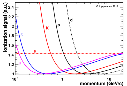
Figure 10: Typical curves of the ionization signal as a function of particle momentum for a number of known charged particles. A parameterization like the one suggested in Ref. [20] was used to calculate the curves.

In practice, only relative values of the deposited energy $\Delta=\Delta(m,\beta)$ are needed to distinguish between different particle species. Because Eq. 8 is not a monotonic function of $\beta$, it is not possible to combine it with Eq. 2 in order to obtain a form $m=m(\Delta,p)$, where $p$ is the momentum of the particle. However, the PID capability becomes obvious by plotting ionization curves $\Delta(m,\beta)$ for a number of charged particles. A description of measured ionization curves based on five parameters is given in Ref. [20] and can be used for this purpose. An example is shown in Fig. 10. By simultaneously measuring $p$ and $\Delta$ for any particle of unknown mass, a point can be drawn on this diagram. The particle is identified when this point can be associated with only one of the curves within the measurement errors. Even in areas where the bands are close, statistical PID methods may be applied.

3.5 Energy resolution and separation power

The resolution in the ionization measurement (energy resolution) $\sigma_{E}$ is given by the variance of the Gaussian distribution of the truncated mean values and is in general proportional to the energy deposit: $\sigma_{E}\propto\Delta$. Using Eq. 4, the separation for two particles $A$ and $B$ with different masses but the same momentum can be calculated as

$$n_{\sigma_{E}}=\frac{\Delta_{A}-\Delta_{B}}{\langle\sigma_{A,B}\rangle}\ .$$ (10)

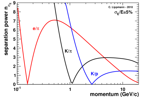
Figure 11: Typical separation power achievable with ionization measurements in a gaseous detector. The ionization curves from Fig. 10 were used together with an assumed energy resolution of 5%.

The average of the two resolutions $\langle\sigma_{A,B}\rangle=(\sigma_{E,A}+\sigma_{E,B})/2$ is used. For the purpose of qualitatively discussing the PID capabilities this approximation is sufficient. For alternative ways to describe the resolution of the PID, refer to Ref. [28].

In Fig. 11 typical particle separations are shown for a gaseous detector with an energy resolution of 5%. As expected, hadron identification works well in the low momentum region. In the minimum ionization region, where hadrons carry momenta around a few GeV/c and the ionization curves are very close, it is likely that the method fails to discriminate the particles. In the region of the relativistic rise moderate identification is possible on a statistical basis.

3.6 Errors affecting the resolution

The operational regime of the particle detector used for the ionization measurements must be chosen such that the measured pulse heights $R$ are exactly proportional to the number of electron/ion (electron/hole) pairs $N_{I}$ created by the energy deposit $\Delta$. The same is true for the signal processing chain. Nevertheless, some effects change the apparent energy deposit and thus limit the energy resolution of the device. They have to be considered on top of the fundamental limit that is given by the statistics of the primary ionization.

• The ionization signal amplitude is determined by the detector (e.g. gas amplification) and by the electronics. An optimal performance can be achieved only if an energy calibration is carried out in order to determine the absolute gain of each channel with high precision.

• Overlapping tracks must be eliminated with some safety margin. This can introduce some limit for a high track density environment like heavy-ion collisions or jets, because the number of ionisation measurements $N_{R}$ entering the truncated mean calculation (Eq. 9) can be considerably reduced by this effect.

• Track independent effects have to be kept under control. For a gaseous device these include the gas density (pressure and temperature) and gas mixture. Electronics effects like noise and baseline shifts have to be taken care of as well.

• On the level of each track, more effects influence the apparent ionization: the detector geometry together with the track orientation influence the amount of ionization charge per sampling layer and can be corrected for. In a gaseous device, attachment of the drifting electrons decreases the ionization signal and requires a correction, which depends on the drift length $z$ through a constant $b$: $R(z)=R\,e^{-bz}$. A similar decrease of the signal as a function of the drift length can be due to diffusion of the drifting primary electron cloud, and can be corrected for as well.

For gaseous detectors, these effects are described in detail in Ref. [20]. An empirical formula exists to estimate the dependence of the energy resolution on the number of measurements $N_{R}$, on the thickness of the sampling layers $x$, and on the gas pressure $P$ [31, 32]:

$$\sigma_{E}=0.41\ N_{R}^{-0.43}(xP)^{-0.32}\ .$$ (11)

The formula was obtained by fits to measured data and includes optimizations such as the truncated mean method and the ones just described. If the ionization measurements along a track were independent, and if no other error sources like electronics noise existed, the resolution would scale as $N_{R}^{-0.5}$. Moreover, the formula shows that for a fixed total length of a detector $x\,N_{R}$, one obtains a better resolution for a finer sampling, provided that the ionization is sufficient in each sampling layer. A comparison of the expected resolutions calculated with Eq. 11 and measured values is given in Ref. [33]. Summaries and examples of performances achieved with gaseous tracking detectors like Drift, Jet or Time Projection Chambers are given in Refs. [20, 32]. Typical values are 4.5 to 7.5%. By increasing the gas pressure, the resolution can be significantly improved, e.g. for the PEP TPC an energy resolution of below 3% was achieved at 8.5 bar. However, at higher pressure the relativistic rise is reduced due to the density effect.

3.7 ALICE Time Projection Chamber

The ALICE TPC [29, 30] (Fig. 12) is the largest gaseous Time Projection Chamber built so far. A TPC is a remarkable example of a detector performing precise tracking and PID through measurements of the energy deposited through ionization. Since it is basically just a large volume filled with a gas, a TPC offers a maximum of active volume with a minimum of radiation length. In a collider experiment like ALICE, the field cage of a TPC is typically divided into two halves separated by a planar central electrode made by a thin membrane. The electrons produced by charged particles crossing the field cage drift towards the two end-caps, where readout detectors are mounted. In general, a gated wire grid is installed directly in front of the readout chambers. When the system is triggered, the gate opens, allowing the passage of the ionization electrons, which create charge avalanches in the readout detectors. Closing the gate assures that the ions created in the avalanche process do not enter the drift volume. Measuring the signals induced on adjacent readout pads makes possible an accurate determination of the position by evaluating the center of gravity. Together with accurate measurements of the arrival time (relative to some external reference such as the collision time of the beams) the complete trajectory of all charged particles traversing the TPC can be determined. Due to the little amount of dead volume and the easy pattern recognition (continuous tracks), TPCs are the best tracking devices for high multiplicity environments, e.g. heavy-ion experiments.

Figure 12: 3D view of the TPC field cage [30]. The high voltage electrode is located at the center of the 5 m long drift volume. The two endplates are divided into 18 sectors holding two readout chambers each.

3.7.1 Field cage and readout chambers

The ALICE TPC is a large-volume TPC with overall “conventional” lay-out but with nearly all other design parameters pushed towards the limits. A comprehensive description can be found in Ref. [30]. The TPC field cage is a hollow cylinder whose axis is aligned with the LHC beam axis and is parallel to the magnetic field. The active volume has an inner radius of about 85 cm, an outer radius of about 250 cm, and an overall length along the beam direction of 500 cm. The central electrode is charged to 100 kV and provides, together with a voltage dividing network at the surface of the outer and inner cylinder, a precise axial electric field of 400 V/cm. To ensure low diffusion of the drifting electrons and a large ion mobility, Ne was chosen as the main component of the counting gas. The gas mixture with 10 % of CO₂ as quencher makes mandatory a very good temperature homogenisation in the drift volume ($\Delta T<0.1$ K), in order to guarantee a homogeneous drift velocity. It is operated at atmospheric pressure.

Wire chambers with cathode pads are used for the readout of the TPC. An optimization of the design for the expected high track density environment implied rather small pad sizes ($4\times 7.5$ mm² in the innermost region). As a consequence, the number of pads is large ($\sim$560 000; for comparison: the ALEPH TPC had 41 000 pads), and the readout chambers have to be operated at rather high gas gains near $10^{4}$.

3.7.2 Front-end electronics

Also for the design of the front-end electronics the key input was the operation in a high track density environment [30]. A signal occupancy as high as 50% can be expected for central Pb–Pb collisions. Due to the large raw data volume (750 MB/event) zero suppression is implemented in the front-end electronics, thus reducing the event sizes to about 300 kB for p–p collisions (no overlying events) and to about 12 MB for Pb–Pb collisions. Signal tail cancellation and baseline correction are performed before the zero suppression in order to preserve the full resolution on the signal features (charge and arrival time). A large dynamic range ensures that the ionization signal of particles can be determined with precision from very low up to high momenta.

3.7.3 PID performance and outlook

A very good energy calibration is fundamental for an optimal PID performance (see Sect. 3.6). In the ALICE TPC, the amplitude of the ionization signal is determined by the gas amplification and the electronics. The absolute gain of each channel is obtained with high precision by periodically releasing radioactive krypton (${}^{83}_{36}$Kr) into the TPC gas system and measuring the well known decay pattern (for more details see  [30]).

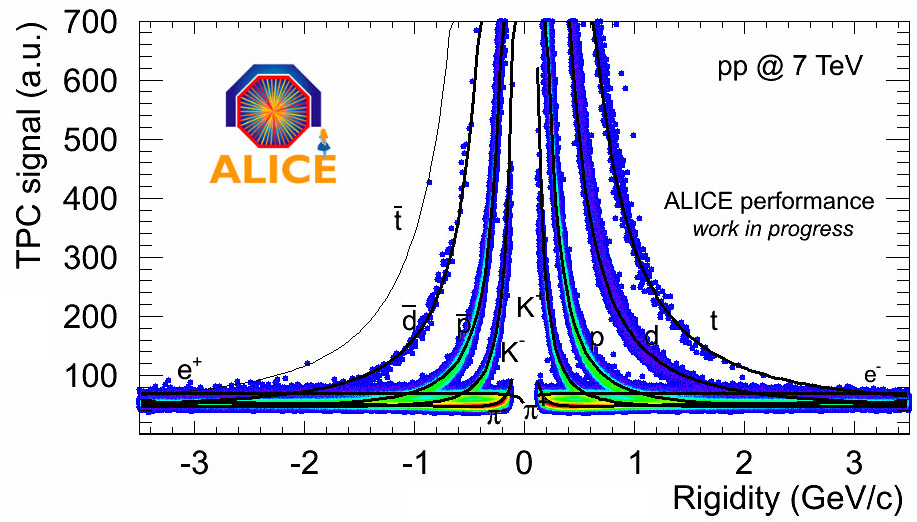
Figure 13: Measured ionization signals of charged particles as a function of the track rigidity (particle momentum divided by charge number). $11\times 10^{6}$ events from a data sample recorded with $\sqrt{s}=7$ TeV p–p collisions provided by the LHC were analysed. The lines correspond to a parameterization of the Bethe-Bloch curve as described in Ref. [20]. Also heavier nuclei like deuterons and tritium and their anti-particles are found.

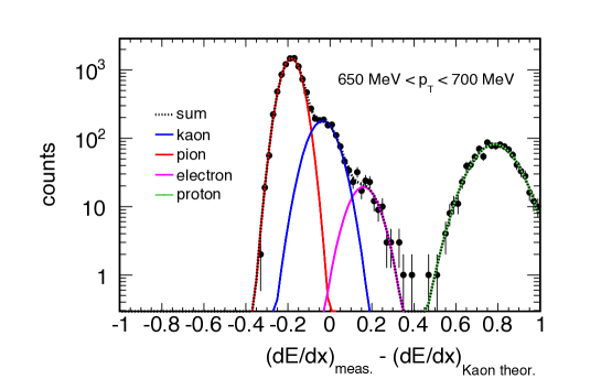
Figure 14: Distribution of the difference between the measured ionization signals and the one expected for Kaons for a momentum slice of 50 MeV/c width. The lines are fits, indicating that a sum of four Gaussians represents well the data. The peak centered at zero reflects the abundance of kaons, the other peaks represent other particle species.

Inside the TPC, the ionization strength of all tracks is sampled on up to 159 pad rows. The energy resolution is 5% for tracks with the maximum number of signals. Fig. 13 shows the ionization signals from $11\times 10^{6}$ events from a data sample recorded with $\sqrt{s}=7$ TeV p–p collisions provided by the LHC. Clearly the different characteristic bands for various particles including deuterons and tritium are visible for particles and anti-particles, respectively. In order to achieve PID in a certain momentum region, histograms are filled and fitted with multiple Gaussians. An example is shown in Fig. 14. For a given ionization signal in this momentum region one can derive the particle yields, which represent the probabilities for the particle to be a kaon, proton, pion or electron.

The ALICE TPC is in nearly continuous data taking mode since more than one year, providing tracking and PID information while the LHC delivers p–p collisions at $\sqrt{s}=7$ TeV. In November 2010 the first Pb–Pb collisions at $\sqrt{s_{NN}}=2.76$ TeV were recorded. The energy resolution of the TPC in these heavy-ion collisions was found to degrade slightly to an average of about 5.3%. This effect is expected due to overlapping signals from neighboring tracks. The energy resolution for the highest multiplicity events falls off by 20% with respect to low multiplicities. Part of the increase is also explained by baseline fluctuations in the electronics due to large hit densities in single channels. These fluctuations can in the future be minimised using the signal tail cancellation and baseline correction features available in the TPC front-end electronics. In the course of the year 2011, higher luminosities will be reached and space charge effects and gating efficiency will have to be accurately evaluated to avoid negative effects on the tracking and ionization sampling.

3.8 Silicon detectors at LHC

At the LHC, the signal amplitude information of the silicon strip (ALICE, ATLAS and CMS) and drift (ALICE) detectors of the tracking systems make possible hadron ID via ionization measurements. However, since in solid media due to a stronger density effect the Fermi plateau is only slightly above the minimum, good $\pi$/K (p/K) separation is achievable only up to 450 MeV/c (up to 1 GeV/c). Again, the energy loss is estimated as a truncated mean in order to minimize the influence of Landau fluctuations. In ALICE, the resolution of the measurement in two layers each of silicon strip and drift detectors is about 11%. In the CMS tracking system, the signal amplitudes from ten layers of silicon strip detectors may be used, but a resolution was not known to the author at the time of writing this review.

3.9 Developments for future TPCs

A TPC at a future linear collider will very likely be read out by micro-pattern devices like GEMs [19] or MicroMegas [34]. Their advantages are the high rate capability and a low ion feedback. Large TPC protopypes with different readout options were built tested [35]. The conventional readout of the micro-pattern device, with mm-sized cathode pads, may actually be replaced by a digital device with pixel sizes of the order 55 $\mu$m. A family of ASIC chips is particularly suited for this purpose: MEDIPIX [36] and its successor TIMEPIX [37], which records also the time. This kind of setup has been shown to detect tracks of minimum ionizing charged particles (MIPs) with excellent single-electron efficiency and unprecedented spatial resolution. In this way, the cluster counting method may be used to assess the energy deposit through ionization: rather than measuring the deposited charge, the number of primary collision clusters are counted. This avoids the problems related to the fluctuation of the energy transfer in single collisions (see Sects. 3.3 and 3.4) and should provide the ultimate resolution of $\sim$2% [38]. Concerning the implementation in a large detector like a TPC, the challenges will include equipping a large active area with the pixelized readout and handling huge amounts of readout channels.

4 Time-of-flight

Time-of-flight (TOF) measurements yield the velocity of a charged particle by measuring the particle flight time $t$ over a given distance along the track trajectory $L$. The particle velocity $\beta=v/c=L/tc$ depends on its mass $m$ and momentum $p$ through

$$\beta=\frac{1}{\sqrt{\left(\frac{mc}{p}\right)^{2}+1}}\ .$$ (12)

Thus, one can calculate the mass $m$ from measurements of $L$, $t$ and $p$:

$$m=\frac{p}{c}\sqrt{\frac{c^{2}t^{2}}{L^{2}}-1}\ .$$ (13)

4.1 Time resolution and separation power

If two particles with masses $m_{A}$ and $m_{B}$, respecively, carry the same momentum, their flight time difference can be calculated as

$$|t_{A}-t_{B}|=\frac{L}{c}\left|\sqrt{1+\left(\frac{m_{A}c}{p}\right)^{2}}-\sqrt{1+\left(\frac{m_{B}c}{p}\right)^{2}}\ \right|\ .$$ (14)

With $p\gg mc$ the approximation $\sqrt{1+(mc/p)^{2}}\approx 1+(mc)^{2}/2p^{2}$ can be used, and with Eq. 4 the separation power becomes

$$n_{\sigma_{TOF}}=\frac{|t_{A}-t_{B}|}{\sigma_{TOF}}=\frac{Lc}{2p^{2}\sigma_{TOF}}|m_{A}^{2}-m_{B}^{2}|\ .$$ (15)

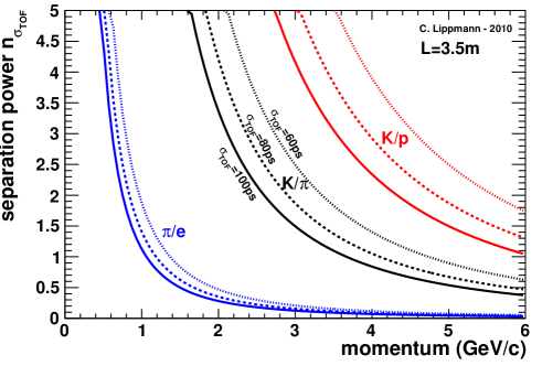
Figure 15: Particle separation with TOF measurements for three different system time resolutions ($\sigma_{TOF}=60$, 80 and 100 ps) and for a track length $L=3.5$ m. Infinitely good precisions on momentum and track length measurements are assumed.

Here $\sigma_{TOF}$ is the resolution of the TOF measurement. Misidentification of particles occurs at higher momenta, where the time difference $|t_{A}-t_{B}|$ becomes comparable to $\sigma_{TOF}$. Assuming a time resolution of 100 ps (60 ps) and requiring a separation of $n_{\sigma_{TOF}}=3$, the upper limits for the momentum are 2.1 GeV/c (2.7 GeV/c) for K/$\pi$ separation and 3.5 GeV/c (4.5 GeV/c) for K/p separation (see Fig. 15). A lower momentum threshold is defined by the curvature of the tracks in the magnetic field. Assuming a path length $L=3.5$ m and a magnetic field of $0.5$ T, only particles with a momentum larger than about $300$ MeV/c reach the TOF wall.

4.2 Errors affecting the resolution

The mass resolution of a TOF measurement is given by:

$$\left(\frac{\mbox{d}m}{m}\right)^{2}=\left(\frac{\mbox{d}p}{p}\right)^{2}+\left(\gamma^{2}\frac{\mbox{d}t}{t}\right)^{2}+\left(\gamma^{2}\frac{\mbox{d}L}{L}\right)^{2}\ .$$ (16)

Since in most cases $\gamma\gg 1$, the mass resolution is predominantly affected by the accuracies in the time and length measurements, rather than by the accuracy of the momentum determination. In general the track length $L$ and the momentum $p$ can be measured with rather good accuracies in the tracking system ($\sigma_{p}/p\approx 1$%, $\sigma_{L}/L\approx 10^{-3}$). The time-of-flight $t$ is measured with a certain accuracy $\sigma_{TOF}$ by a dedicated detector system. A TOF measurement always consists of two time measurements: $t=t_{1}-t_{0}$. The event start time $t_{0}$ is measured with accuracy $\sigma_{t_{0}}$. The stop time $t_{1}>t_{0}$ is measured with accuracy $\sigma_{t_{1}}$ by the actual TOF detector, usually a large area detector system some distance away from the interaction region. The overall TOF resolution is then given by $\sigma_{TOF}^{2}=\sigma_{t_{0}}^{2}+\sigma_{t_{1}}^{2}$.

4.3 Resistive Plate Chambers for time-of-flight measurements

In order to optimise a TOF system the resolution $\sigma_{TOF}$ has to be improved. In current experiments for subnuclear research, detectors using scintillation (the property of luminescence when excited by ionizing radiation) are very commonly used due to their good time resolution. However, as the experiments have gradually increased in size, and since the readout of scintillator detectors is expensive, the cost per area became an important issue. The Resistive Plate Chamber (RPC) was found to provide a simpler technology at a much lower price. RPCs can be seen as the successor of the metallic Parallel Plate Avalanche Counters, overcoming their disadvantage of being very vulnerable to the destructive energy released by possible discharges or sparks. The electrode plates of RPCs are made from a resistive material, which effectively restricts excessive signals or discharges to a well localised area of the detector. As a side effect, all charges cause a local drop of the electric field in the gas gap and in this spot the detector becomes insensitive to further traversing particles for a time of the order of the relaxation time $\tau=\rho\,\varepsilon_{0}\varepsilon_{r}$, where $\varepsilon_{0}$ is the dielectric constant and $\rho$ and $\varepsilon_{r}$ are the volume resistivity and the relative permittivity of the resistive material. Even though the remaining counter area is still sensitive to particles, a limit to the overall rate capability is introduced through this effect. In general, accurate time measurements are feasible up to charged particle rates of a few kHz/cm², which is acceptable for many purposes (compare to Sect. 4.7).

The RPC design was improved by introducing the concept of multiple gaps (Multi gap Resistive Plate Chamber, MRPC [39]), resulting in an increase of detection efficiency. Reducing the individual gap sizes [40], while at the same time increasing the electric field, resulted in what is called the Timing RPC, a low cost detector with a time resolution comparable to that of scintillators. The space resolution can be chosen by different sizes of the readout strips.

4.4 Detector physics of Resisitive Plate Chambers

The physics of avalanches in RPCs is very complex, even though the simple geometry of the device would not suggest so. During the development of large area RPC systems for the LHC experiments, the detector physics of RPCs was therefore studied in detail [41, 42, 43, 44, 45, 46, 47, 48]. The good detection efficiency of (single gap) RPCs is explained by the very large gas gain. A very strong space charge effect reduces the avalanche charges by many orders of magnitude. Detailed simulations show that the space charge field inside the avalanches actually reaches the same magnitude as the applied electric field.

The very good time resolution of RPCs is due to the strong uniform electric field, which provokes the avalanche process immediately after primary ionization is deposited in the gas volume. As a consequence, the intrinsic detector time resolution (no electronics) is determined by the avalanche statistics, and can be estimated using a simple formula (for one gas gap):

$$\sigma_{Intr}\approx\frac{1.28}{(\alpha_{g}-\eta_{g})v_{D}}\ .$$ (17)

Here $\alpha_{g}$ and $\eta_{g}$ are the Townsend and attachment coefficients of the gas mixture and $v_{D}$ is the the drift velocity of electrons. Typical operational parameters [41] for Timing RPCs are $\alpha_{g}=123$ mm^-1, $\eta_{g}=10.5$ mm^-1 and $v_{D}=210$ $\mu$m ns^-1. For these values an intrinsic time resolution of $\sigma_{Intr}=50$ ps is obtained for a single gap. By increasing the number of gaps $n$, the resolution can be improved, but for small values of $n$ the improvement is not following a simple $1/\sqrt{n}$ scaling, because it is dominated by the gap which has the largest signal [41]. For $n=10$ gaps a resolution of $\sigma_{Intr}=20$ ps is feasible.

The drop of the electric field in the gas gap at high particle rates affects efficiency and time resolution. It may be calculated in a simple way by assuming the particle flux to be a DC current that causes a voltage drop when it passes through the resistive plate. For a single gap of width $b$ the average field reduction is:

$$\langle\Delta E\rangle=\rho\frac{a}{b}\Phi Q\ ,$$ (18)

where $\rho$ and $a$ are the volume resistivity and thickness of the resistive electrode material and $\Phi$ is the particle flux per area. $Q$ is the avalanche charge, which of course depends itself on the field reduction, and has thus to be found in an iterative procedure. An approximate analytic expression for the field fluctuations around $\langle\Delta E\rangle$ is given in Ref. [43].

4.5 ALICE time-of-flight detector

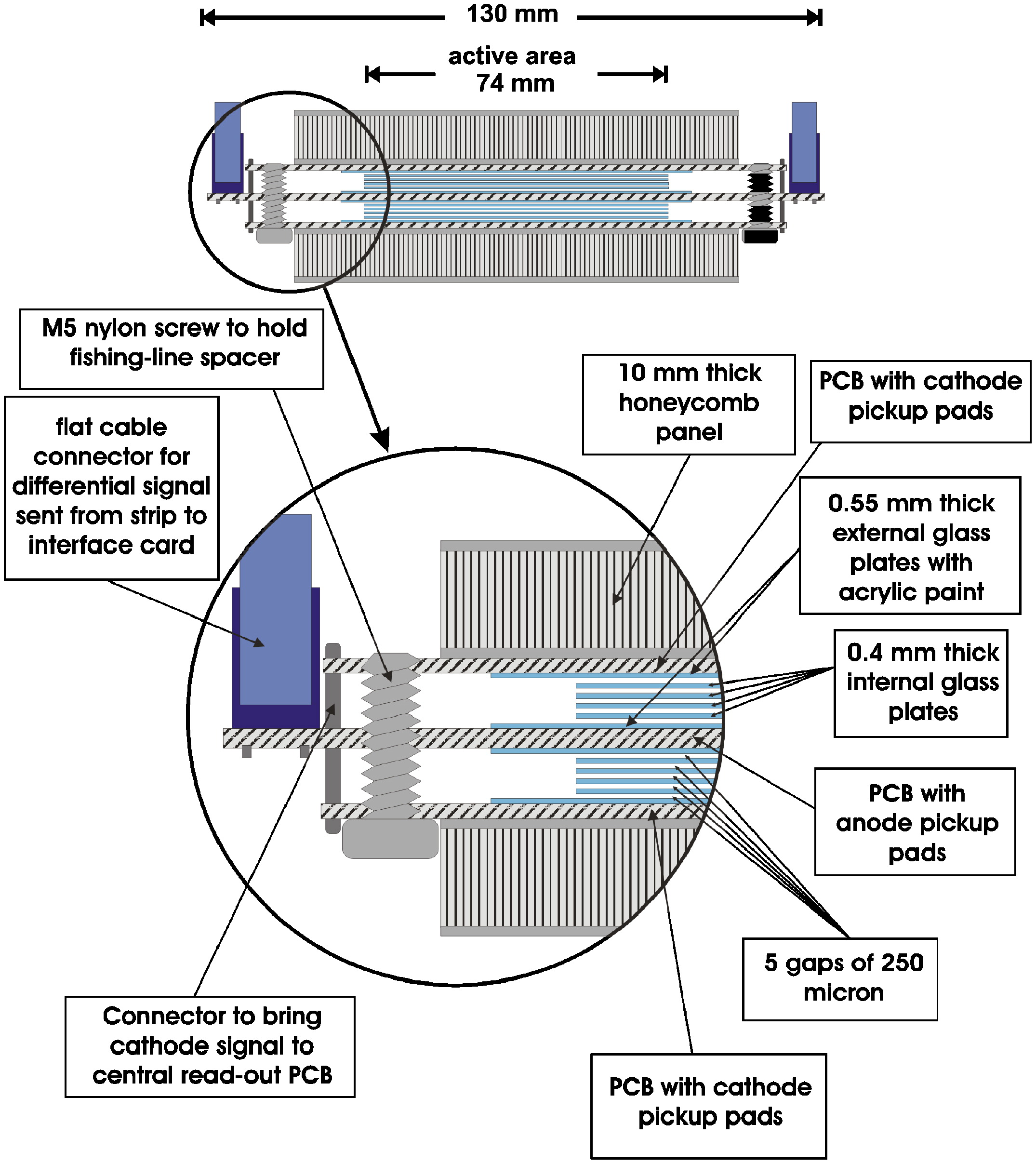
Figure 16: Cross-section of an ALICE MRPC [13].

In specific momentum ranges, the PID signals from the ALICE TPC can not be used to separate kaons, pions and protons, because the ionization curves are very close or overlap (see also Fig. 5). The NA49 and STAR experiments have shown [49, 50] how the hadron identification capability may be extended by combining the PID informations from TPC and TOF. Moreover, a reliable identification of electrons is possible up to a few GeV/c in this way, since the hadrons (which for a given momentum are slower) can be eliminated with a cut on the particle velocity.

The ALICE TOF detector [51] is based on MRPCs. 91 MRPCs each are assembled into gas tight modules in 18 azimuthal sectors (supermodules) surrounding the ALICE TPC and TRD (see Fig. 8). The supermodules have about 9 m length, covering the pseudo-rapidity interval $|\eta|<0.9$. More than 150 000 readout pads with size $2.5\times 3.5$ cm² cover an area of about 150 m². The gas mixture in the ten 250 $\mu$m thin gas gaps is 90% C₂H₂ F₄, 5% C₄H₁₀, 5% SF₆. A cross-section through one MRPC is shown in Fig. 16.

4.5.1 Time resolution

The design goal for the ALICE TOF was to reach a global TOF resolution of $\sigma_{TOF}\approx 100$ ps. The following contributions have to be considered:

$$\sigma_{TOF}^{2}\ =\ \sigma_{t_{0}}^{2}+\sigma_{t_{1}}^{2}\ =\ \sigma_{t_{0}}^{2}+\sigma_{Intr}^{2}+\sigma_{Elec}^{2}+\sigma_{Clock}^{2}+\sigma_{Cal}^{2}\ .$$ (19)

Here $\sigma_{t_{0}}$ is the uncertainty in the absolute time of the collision, $\sigma_{Intr}$ is the intrinsic time resolution of the detector technology ($\sim$20 ps) and $\sigma_{Elec}$ combines the intrinsic time jitter of the amplification electronics ($\sim$20 ps) and of the time-to-digital conversion ($\sim$30 ps). $\sigma_{Clock}$ is an uncertainty arising from the distribution of the digital clock from the LHC to the experiment ($\sim$15 ps) and through the electronics chain ($\sim$10 ps). Finally, a contribution $\sigma_{Cal}$ includes all effects that can be parametrised and that are thus accessible to calibration methods in order to be minimised. These are mainly

1. the relative timing of the different channels given by cable lengths (time offset),

2. the influence of the finite rise time of the ampliflying electronics (time slewing) and

3. the influence of the impact position of the particle through signal propagation delays on the pad (time walk).

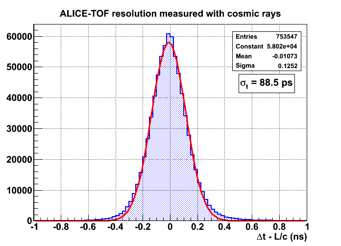
Figure 17: TOF measurements with a cosmic data sample from the year 2009. Since the start and stop time were both measured with the ALICE TOF, the resolution of a single time measurement is obtained from the histogram by dividing its width by $\sqrt{2}$. The resulting resolution of 88.5 ps corresponds to $\sigma_{t_{1}}$ from Eq. 19.

It is forseen that the contribution $\sigma_{Cal}$ can be kept below 30 ps [16]. Already with the limited statistics available from cosmics data samples before the start of the LHC it was possible to reach a value of $\sigma_{Cal}=70$ ps. The resolution $\sigma_{t_{1}}$ with this “intermediate calibration” (compare to Tab. 2) is shown in Fig. 17.

The absolute time of the collision $t_{0}$ is fluctuating with respect to the nominal time signal from the LHC according to a Gaussian distribution with a $\sigma$ of about 140 ps. This is due to the finite length of the colliding bunches of particles. In ALICE, $t_{0}$ is precisely measured by a dedicated detector (T0) [13], which reduces this uncertainty to $\sigma_{t_{0}}=50$ ps.

Table 2: Overall TOF resolution together with the two main contributions $\sigma_{t_{0}}$ and $\sigma_{Cal}$.

$\sigma_{TOF}$	$\sigma_{t_{0}}$	$\sigma_{Cal}$	Remark
100	50	70	proton collisions, intermediate calibration
80	50	30	proton collisions, optimal calibration
65	10	30	Pb–Pb collisions, optimal calibration

With the much larger statistics that is available from data samples with collisions provided by the LHC, the work now focuses on reducing the contribution $\sigma_{Cal}$. A further improvement can be achieved for high multiplicity Pb–Pb events, where the accuracy of the event start time measurement is expected to improve to $\sigma_{t_{0}}=10$ ps. In that case an overall system resolution $\sigma_{TOF}=65$ ps is possible (compare to Tab. 2).

4.5.2 PID performance and outlook

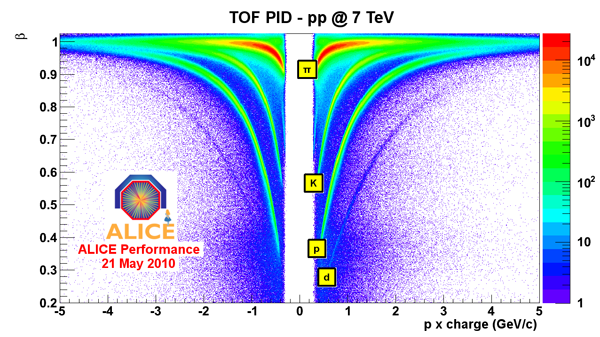
Figure 18: Velocity $\beta=v/c$ as measured with the ALICE TOF detector as a function of the particle momentum $p$ multiplied with the particle charge number $Z$ for a data sample taken with $\sqrt{s}=7$ TeV collisions provided by the LHC in the year 2010. No data is available for momenta $\lesssim$300 MeV/c, since these particles do not reach the detector due to the curvature of their tracks in the magnetic field.

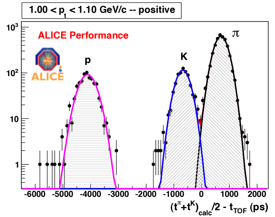
Figure 19: Histogram of the TOF signal for a given momentum window of 100 MeV/c width. The data sample was recorded with $\sqrt{s}=900$ GeV p–p collisions provided by the LHC. The lines are fits to the data, indicating that a sum of three Gaussians well represents the data.

Fig. 18 shows the correlation between the track momentum measured by the ALICE tracking detectors and the velocity $\beta$ as measured by the TOF system. The data were recorded during the first $\sqrt{s}=7$ TeV p–p collisions in 2010 and clearly show two times four bands corresponding to four particle species and their corresponding anti-particles. Data outside these bands indicates errors in the association of tracks to TOF PID signals. A particle is identified when the corresponding point in the diagram of Fig. 18 can be associated with only one theoretical curve (Eq. 12) within the measurement errors. For certain momentum regions histograms are filled and fitted with multiple Gaussians, similar to the procedure described in Sect. 3.7. An example is shown in Fig. 19. For a given TOF measurement one can derive the particle yields, which represent the probabilities for the particle to be a kaon, proton, pion or electron. The power of combining TOF and ionization measurements for PID is demonstrated for in Fig. 20.

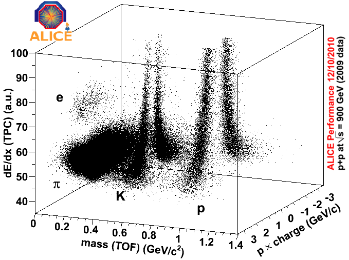
Figure 20: Demonstration of ALICE’s PID capabilities by combining the ionization measurements in the TPC and the mass calculated using the TOF signal. Electrons, pions, kaons and protons are clearly visible in a wide momentum range. The data sample was recorded with $\sqrt{s}=900$ GeV p–p collisions provided by the LHC.

4.6 Other TOF detectors

RPCs have found applications in many particle physics experiments in many variations, as can be seen in the proceedings of the RPC workshop series [52, 53, 54, 55, 56, 57]. The STAR experiment has installed a large area (64 m²) TOF system similar to the ALICE TOF in their barrel, surrounding the TPC [58, 59]. The modules have six gas gaps of 220 $\mu$m width and are filled with a gas mixture of 95% C₂H₂F₄ and 5% i-C₄H₁₀. The STAR experiment also plans to install a Muon Telescope Detector (MTD) based on Timing RPCs to identify muons [60]. The FOPI experiment has upgraded their TOF system in 2007 by installing Multistrip Multigap Resistive Plate Chambers (MMRPCs) with 8 gaps of 220 $\mu$m [61]. For the HADES experiment a similar upgrade of the inner TOF wall is planned for the near future [62].

4.7 Developments for future TOF systems

Driven by the environment in which TOF systems are planned to be operated in future experiments, a number of R&D projects currently address the rate limitation of Timing RPCs. The requirements for the TOF wall of the CBM experiment, for example, include a rate capability up to 25 kHz/cm² with a time resolution of 80 ps on a large system (120m²) [63]. The effective drop of the operating voltage at larger rates (see Sect. 4.3) can be reduced either by lower electrode resistivity or by thinner electrode plates. Different electrode materials are being explored, including low-resistive phosphate and silicate glass [64, 65]. With electrodes made from ceramics the practical feasibility of accurate timing measurements with RPCs at rates up to 500 kHz/cm² was established in test beams [66, 67].

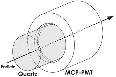
Figure 21: Schematic drawing of a TOF counter based on a MCP-PMT [69]. The MCP-PMT actually detects Cherenkov photons emitted in the quartz glass entrance window and has a very good time resolution.

TOF measurements with charged particles can also be carried out using Micro-Channel Plate (MCP) Photo Multiplier Tubes (PMTs, see Fig. 21)), which allow time measurements with a few ps precision. The MCP-PMT actually detects Cherenkov photons emitted in the entrance window of the PMT (for details on Cherenkov radiation see Sect. 5) [68]. Time resolutions of $\sigma_{t_{1}}\approx 6$ ps (with an intrinsic resolution of the detector of $\sigma_{Intr}<5$ ps) were observed in test beams [69, 70]. At this scale, the resolution of the measurement of the event start time $\sigma_{t_{0}}$ becomes dominant and must be minimised as well. It remains to be shown that this technology can be implemented on large surfaces at an affordable price and can thus compete with MRPCs.

5 Cherenkov imaging

In 1958 P. A. C̆erenkov, I. Y. Tamm and I. M. Frank were awarded with the Nobel Prize in physics for the discovery and interpretation of the Cherenkov effect. Cherenkov radiation is a shock wave resulting from a charged particle moving through a material faster than the velocity of light in the material. The Cherenkov radiation propagates with a characteristic angle with respect to the particle track $\Theta_{C}$, that depends on the particle velocity:

$$\cos(\Theta_{C})=\frac{1}{\beta n}\ ,$$ (20)

where $n$ is the refractive index of the material. In general, the refractive index varies with the photon energy: $n=n(E)$ (chromatic dispersion). Since $|\cos(\Theta_{C})|\leq 1$, Cherenkov radiation is only emitted above a threshold velocity $\beta_{t}=1/n$ and $\gamma_{t}=1/(1-\beta_{t}^{2})^{1/2}$.

In general, Cherenkov detectors contain two main elements: a radiator through which charged particles pass (a transparent dielectric medium) and a photon detector. The number of photoelectrons ($N_{p.e.}$) detected in a given device can be approximated as [23]

$$N_{p.e.}\approx N_{0}z^{2}L\sin^{2}(\Theta_{C})\ ,$$ (21)

where $L$ is the path length of the particles through the radiator, $ze$ is the particle charge and $N_{0}$ is a quantity called the quality factor or figure of merit. As Cherenkov radiation is a weak source of photons, the light transmission, collection and detection must be as efficient as possible. These parameters are contained in $N_{0}$, as well as the photon collection and detection efficiencies of the photon detector. Typical values of $N_{0}$ are between 30 and 180 cm^-1. Three different types of Cherenkov counters can be distinguished:

1. Threshold counters measure the intensity of the Cherenkov radiation and are used to detect particles with velocities exceeding the threshold $\beta_{t}$. A rough estimate of the particle’s velocity above the threshold is given by the pulse height measured in the photon detector.

2. Differential counters focus only Cherenkov photons with a certain emission angle onto the detector and in this way detect particles in a narrow interval of velocities.

3. Imaging Cherenkov detectors make maximum use of the available information (Cherenkov angle and number of photons) and can be divided in two main categories: RICH (Ring Imaging CHerenkov) and DIRC (Detection of Internally Reflected Cherenkov light) devices.

In this paper the focus lies on RICH devices, since the detectors used at the LHC experiments and discussed here all fall into this category.

5.1 Cherenkov ring imaging

RICH detectors resolve the ring shaped image of the focused Cherenkov radiation. From the knowledge of the particle momentum $p$ and Cherenkov angle $\Theta_{C}$ a determination of the mass of the charged particle is possible. Combining Eqs. 12 and 20 yields

$$m=\frac{p}{c}\sqrt{n^{2}\cos^{2}(\Theta_{C})-1}\ .$$ (22)

In a RICH device, the Cherenkov radiation is emitted in the radiator and collected by a photon detector, usually after being transmitted by optical means. The first RICH was developed by A. Roberts in 1960 [71]. The particular design was limited by small angular acceptance and surface area and by low quantum and single electron counting efficiencies. These problems were overcome by J. Seguinot et al. in 1977 [72]: A wire chamber was converted into an efficient single photon detector by adding a photosensitive molecule into the gas mixture and replacing one of the cathode planes by a wire mesh and a UV transparent window.

5.1.1 Radiator

A RICH detector is designed to measure velocities in a specified momentum range by using a Cherenkov radiator with refractive index $n$ chosen such that the Cherenkov angle varies with velocity, from threshold to the highest anticipated momentum. The thickness $L$ of the radiator is adjusted in order to assure a sufficient number of photoelectrons for the given momentum range (see Eq. 21). Two common RICH designs can be distinguished, according to the value of $n$:

1. If a dense medium (large $n$) is used, only a thin radiator layer ($\sim$1 cm) is required to emit a sufficient number of Cherenkov photons. The photon detector is located some distance away behind the radiator (expansion gap, usually about 5 to 10 cm), allowing the light cone to expand and form the characteristic ring-shaped image. A detector designed in such a way is called proximity-focusing (i.e., the focusing is achieved by limiting the emission region of the radiation). An example is shown in Fig. 22.

2. If a gaseous medium ($n\approx 1$) is used, particles have to pass a thicker layer ($\gtrsim$50 cm) in order to emit a sufficient number of Cherenkov photons. In general, fluorocarbon gases are chosen because they have a low chromatic dispersion (i.e. $n$ does not depend strongly on the photon energy). The light is focused by spherical or parabolic mirrors onto the photon detectors where ring-shaped images are formed. An example is shown in Fig. 24.

5.1.2 Optics

The quality of the optics of a RICH system influences the precision in the Cherenkov angle measurement and the figure of merit $N_{0}$. Mirrors should have high reflectivity to avoid photon loss. Traditional constructions use a glass substrate with coating of Al for the reflective surface and MgF₂ or SiO₂ for protection. Such mirrors achieve values for the reflectivity of $\sim$90%. For applications where a minimum of material budget is required, mirrors based on carbon fibre or Be substrates are used (see e.g.  [73] and [74]).

5.1.3 Photon detection

Cherenkov photons are converted to photoelectrons in photocathodes, typically made from CsI or bialkali with low work functions. The photon detection efficiency for a given photon detector is the product of the quantum efficiency (the probability that an incident photon produces a photoelectron, typically 20 to 30%) and the collection efficiency (the efficiency for detecting the photoelectron, typically 80 to 90%). Photon detectors for RICH systems generally fall in two categories: wire chambers with CsI coated cathode pads or detectors based on vacuum tubes with bialkali photocathodes. Examples of both categories are described in the following (Sects. 5.3 and 5.4). Low noise is a general requirement to ensure the detection of single photoelectrons. Recently also the readout speed of the devices became increasingly important in order to cope with the highest event rates.

5.1.4 Pattern recognition

In the busy environment of hadronic collisions (such as at the LHC) many tracks may pass through the detector, which leads to overlapping rings. The assignment of photon hits to rings and the association of rings to tracks requires pattern recognition. Most approaches rely on the use of the particle track prolonged from the tracking system to seed the ring search. After transformation through the optics of the RICH, the track will lie inside the ring. For RICH designs where the track is known to always point through the ring center the ring search is actually quite simple and corresponds to the search for a peak in the number of photon hits versus radius from the track. In any case, the ring search efficiency needs to be studied in detail using Monte Carlo methods.

5.2 Angular resolution and separation power

The particle velocity $\beta$ can be calculated from the reconstructed Cherenkov angle according to Eq. 20. The resolution of the velocity measurement is given by [23, 75]

$$\frac{\sigma_{\beta}}{\beta}=\tan(\Theta_{C})\,\sigma_{\Theta_{C}}\ ,$$ (23)

where $\sigma_{\Theta_{C}}$ is the resolution of the Cherenkov angle measurement. In practical counters $\sigma_{\Theta_{C}}$ varies between about 0.1 and 5 mrad depending on the size, radiator material and length, and on the photon detector. The Cherenkov angle is determined by $N_{p.e.}$ measurements of the angles of emission of the single Cherenkov photons. With the average angular resolution for the angle measurement for the single photoelectron $\sigma_{\Theta_{i}}$, the total resolution becomes

$$\sigma_{\Theta_{C}}^{2}=\left(\frac{\sigma_{\Theta_{i}}}{\sqrt{N_{p.e.}}}\right)^{2}+\sigma_{Glob}^{2}\ .$$ (24)

The term $\sigma_{Glob}$ combines all contributions that are independent of the single photoelectron measurement. These include misalignment of the photon detector modules, the resolution deterioration due to multiple scattering and background hits and errors in the calculation of the reconstructed track parameters. For the single photoelectron angular resolution, the following contributions have to be considered:

$$\sigma_{\Theta_{i}}^{2}\ =\ \sigma_{EP}^{2}+\sigma_{Chro}^{2}+\sigma_{Det}^{2}\ ,$$ (25)

where

1. $\sigma_{EP}$ is the geometrical error related to the emission point. For proximity-focusing devices the emission point is not known, and all photons are in general treated as if emitted at one point of the track through the radiator. This leads to some smearing of the reconstructed angle. Also for other designs the geometry of the optics (e.g. the tilting of the focusing mirror) can lead to a dependence of the image of a Cherenkov photon on its emission point on the track.

2. $\sigma_{Chro}$ is the error due to the chromatic dispersion of the radiators. Cherenkov photons are emitted with a distribution of wavelengths. Since the refractive index varies with wavelength, the Cherenkov angle is also spread.

3. $\sigma_{Det}$ is the error introduced by the finite granularity of the detector (e.g. pixel or pad size), which limits the precision.

These contributions depend on the signal-to-noise ratio (detector gain) and can be a function of the impact angles of the track with respect to the detector surface.

Assuming two particles of momentum $p$ and mass $m_{A}$ and $m_{B}$, respectively, then the Cherenkov angles $\Theta_{C,A}$ and $\Theta_{C,B}$ are measured. The resolution $\sigma_{\Theta_{C}}$ determines the momentum range over which the two particles can be separated, since the Cherenkov angle saturates and thus the ring radii get closer. Using Eq. 4, the separation power can be calculated as

$$n_{\sigma_{\Theta_{C}}}=\frac{\Theta_{C,A}-\Theta_{C,B}}{\langle\sigma_{\Theta_{C}}\rangle}\ .$$ (26)

For velocities $\beta\approx 1$ well above threshold $\beta_{t}$, the separation power can be approximated as [23]

$$n_{\sigma_{\Theta_{C}}}\approx\frac{c^{2}}{2p^{2}\langle\sigma_{\Theta_{C}}\rangle\sqrt{n^{2}-1}}|m_{B}^{2}-m_{A}^{2}|\ .$$ (27)

Note the similarity to the formula for the separation power using the TOF technique (Eq. 15). In the case of a RICH there is however an additional factor of $1/\sqrt{n^{2}-1}$, which allows to adjust the detector configuration in order to achieve the desired momentum coverage. Together with Eqs. 21 and 24 it is clear that the best separation is achievable by designing counters able to detect the maximum number of photons (large $N_{0}$) with the best single photoelectron angular resolution (small $\sigma_{\Theta_{i}}$).

5.3 ALICE HMPID detector

The ALICE High-Momentum Particle IDentificaton (HMPID) [76] was designed to enhance the PID capabilities of the ALICE experiment. The HMPID is a RICH system optimised to extend the useful range for K/$\pi$ and K/p discrimination up to 3 GeV/c and 5 GeV/c, respectively. Moreover, light nuclei (alpha particles, deuterons, tritium) can be identified. The HMPID is a single-arm array with a reduced geometrical acceptance of $|\eta|<0.6$ in pseudo-rapidity and 1.2${}^{\circ}<\phi<58.8^{\circ}$ in azimuth. The detector is based on proximity-focusing RICH counters and consists of an array of seven identical modules of about $1.5\times 1.5$ m² each.

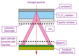
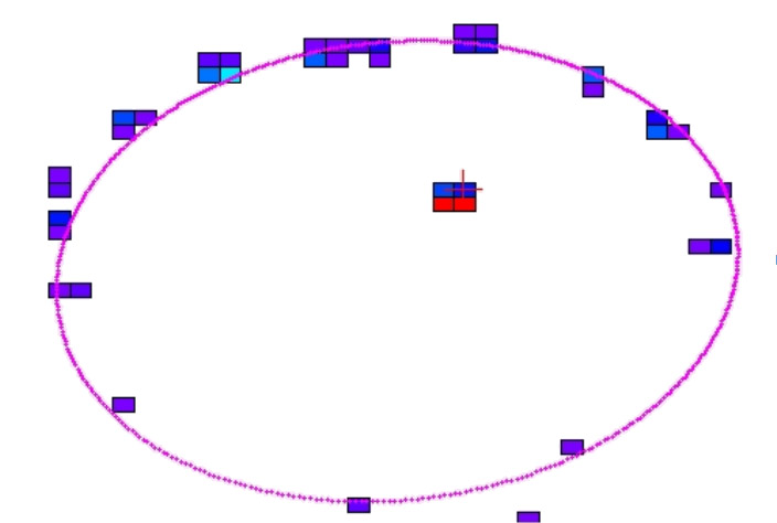
Figure 22: Left image: schematic layout of an ALICE HMPID module, showing radiator, expansion gap and photon detector [13]. Right image: example ring as seen by the HMPID. The ring has a radius of the order 10 cm, but its shape is distorted due to the impact angle of the particle.

5.3.1 Radiator

In each module, the radiator is a 1.5 cm thick layer of C₆F₁₄ liquid (perfluorohexane) with an index of refraction of $n\approx 1.3$ at $\lambda=175$ nm. The material has a low chromaticity, keeping small the corresponding term in the angular resolution. The expansion gap has 8 cm thickness.

5.3.2 Photon detector

Cherenkov photons are detected by wire chambers with a thin layer (300 nm) of CsI deposited onto the cathode pad plane. CsI is a stable alkali halide crystal with high quantum efficiency of 25% at a wavelength of 175 nm [77, 78]. The total size of the photosensitive area is 11 m², making the HMPID the largest scale application of the CsI technique so far. The expansion gap and wire chambers are filled with CH₄ at atmospheric pressure. The size of the cathod pads is $8\times 8.4$ mm².

5.3.3 Performance and outlook

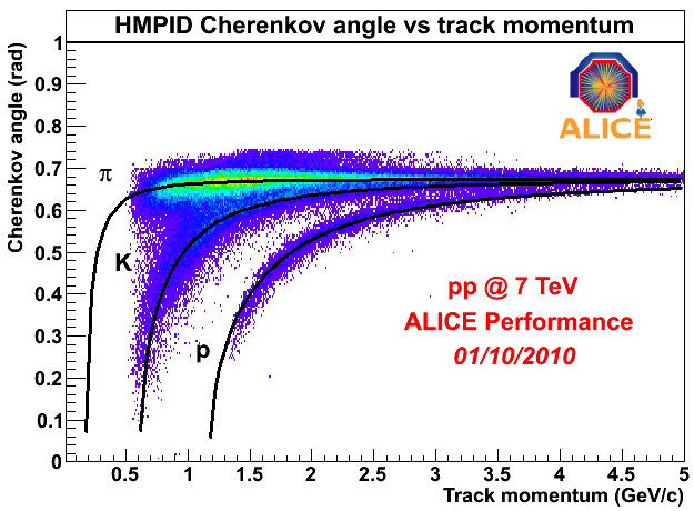
Figure 23: Dependence of the Cherenkov angle measured by the ALICE HMPID on the particle momentum. The lines are the theoretical curves calculated using Eq. 20 with the refractive index $n=1.3$. No data is available for momenta below about 600 MeV/c, because only particles with higher momenta reach the detector.

The identification of charged particles with known momenta in the HMPID requires their tracks to be extrapolated from the central tracking devices (ITS, TPC and TRD) and associated with an ionization cluster in the HMPID. For the particular setup of a proximity-focusing RICH, the shape of the ring is determined by the incident angle of the particle track (see Fig. 22), which makes the Cherenkov angle reconstruction quite complex. With a single photoelectron angular resolution $\sigma_{\Theta_{i}}\lesssim 12$ mrad for perpendicular tracks [79], the resolution in the reconstruction of the Cherenkov angle is $\sigma_{\Theta_{C}}\approx 3.5$ mrad (for perpendicular tracks and for $\beta\approx 1$). Measured Cherenkov angles for different particles as a function of momentum are shown in Fig. 23. In the high multiplicity environment of Pb–Pb collisions the detection of Cherenkov rings is more challenging and the angular resolution is slightly worse. However, at the time of writing this article no quantitative results from the first heavy-ion data taking period (November 2010) were available to the author yet.

In order to extend the PID range up to around 30 GeV/c, it was proposed to add a Very High Momentum PID (VHMPID) detector to ALICE [80]. The physics requirements have driven the choice towards a RICH detector using a C₄F₁₀ gaseous radiator ($n=1.0014$) with length $L=80$ cm in a focusing configuration using a spherical mirror.

5.4 LHCb RICH

The LHCb experiment was introduced in Sect. 2.3. Important for the underlying physics goals is a K/$\pi$ separation in the momentum range $2\lesssim p\lesssim$100 GeV/c, which is achieved by two RICH detectors [18, 81, 82]. RICH1 and RICH2 are both characterised by a design that places the photodetectors outside the acceptance of the LHCb spectrometer in order to limit the degradation of the resolution of the tracking systems due to interaction with the detector material. A set of spherical and flat mirrors projects the Cherenkov light onto the detector plane. The spherical mirrors are placed inside the spectrometer acceptance and special care was taken to minimise the fraction of radiation length while at the same time ensuring the mechanical integrity of the optics. The spherical mirror of RICH1 is made from carbon fibre, with thickness corresponding to only about $0,01\,X_{0}$. The schematic layout of RICH1 is shown in Fig. 24.

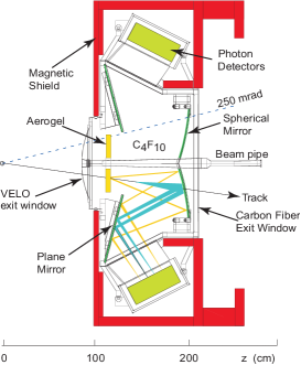
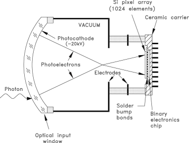
Figure 24: Left image: schematic layout of the LHCb RICH1 detector. The acceptance of $\pm 250$mrad is indicated. Right image: schematic view of an HPD of the LHCb RICH system. Both figures are taken from Ref. [18].

5.4.1 Radiators

In both detectors gaseous radiators are used. In RICH1 a second, denser radiator made from silica aerogel is installed in addition. Together the three radiators cover the large momentum range that is required. The parameters of the three radiators are summarised in Tab. 3. The Cherenkov angles for the three different materials and for different particles as a function of the momentum are shown in Fig. 25.

Table 3: Some parameters of the LHCb RICH detectors. The quoted measured angular resolutions [86] are for the preliminary alignment available from the first data sample with p–p collisions at $\sqrt{s}=7$ TeV.

		RICH1		RICH2
		Silica aerogel	C4F10	CF4
Momentum range [GeV/c]		$\leq$10	$10\lesssim p\lesssim 60$	$16\lesssim p\lesssim$100
Angular acceptance [mrad]	vertical	$\pm 25$ to $\pm 250$		$\pm 15$ to $\pm 100$
	horizontal	$\pm 25$ to $\pm 300$		$\pm 15$ to $\pm 120$
Radiator length [cm]		5	95	180
Refractive index $n$		1.03 (1.037)	1.0014	1.0005
Maximum Cherenkov angle [mrad]		242 (268)	53	32
Expected photon yield at $\beta\approx 1$		6.7	30.3	21.9
$\sigma_{\Theta_{C}}$ [mrad]	expected	2.6	1.57	0.67
	measured	$\sim$7.5	2.18	0.91

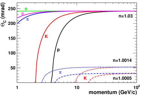
Figure 25: Cherenkov angles as a function of momentum for different particle species and for the three different values of the refractive index $n$ corresponding to the three radiator materials used in the LHCb RICH setup.

5.4.2 Photon detectors

For the photon detectors the requirements are very demanding: they should be sensitive to single photons with high efficiency, cover a large area (about 4 m²) with a granularity of about $2.5\times 2.5$ mm², and have readout fast enough to match the LHC bunch-crossing separation of 25 ns. LHCb chose Hybrid Photon Detectors (HPD) [85], which combine the photon sensitivity of vacuum PMTs with the excellent spatial and energy resolutions of silicon sensors. The conversion of the photoelectrons takes place in the quartz window with bialkali photocathode and they are then accelerated through a potential difference of about 20 kV and detected by a silicon pixel chip. HPDs are sensitive to single photons in the wavelength range from 200 to 600 nm with a quantum efficiency of about 31%. About 65% of the detection plane is covered with read out pixels.

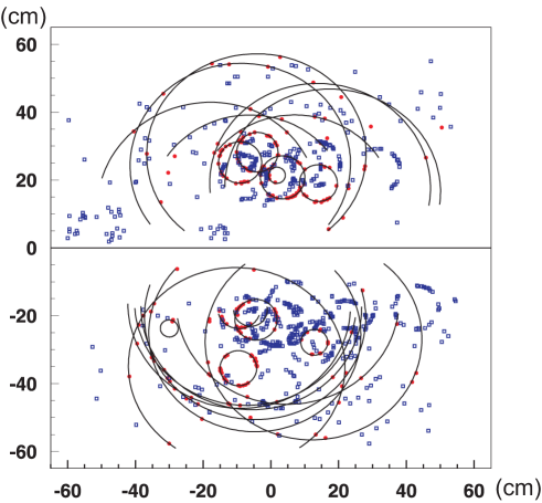
Figure 26: Typical, simulated LHCb event in the RICH1 detector [18]. The data from the two photodetector planes are drawn in the upper and lower halves.

The photoelectron trajectories are deformed by the magnetic field of the large LHCb dipole magnet. This effect can be corrected by comparing reproducible light-spot patterns, that are illuminated onto the photon detector plane, with magnetic field on and off.

5.4.3 Performance

A typical (simulated) LHCb event in the RICH1 detector is shown in Fig. 26. The expected single photoelectron angular resolutions are given in Tab. 3. After the first alignment carried out with data from p–p collisions, the achieved resolutions are already approaching those values [86]. For the aerogel radiator, the refractive index was found to change from its initial value of $n=1.03$ to $n=1.037$ in the experiment, which is probably explained by absorption of C₄F₁₀, since the aerogel material is not sealed from the gas volume. As a consequence, the measured photon yield and angular resolution are slightly worse than expected. Using the expected values, the separation power $n_{\sigma_{\Theta_{C}}}$ can be calculated for all three radiator materials according to Eq. 26. The results are shown in Fig. 27.

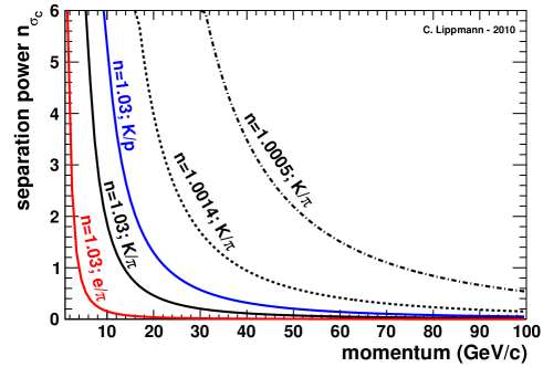
Figure 27: Particle separation achievable with Cherenkov angle measurements for the three different radiator materials used in the LHCb RICH detectors. As Cherenkov angular resolutions the expected values from Tab. 3 were used.

Particle identification with the LHCb RICH system uses a global pattern recognition and maximum likelihood method. All found tracks in the event and all three radiators are considered simultaneously and the observed pattern of hit pixels in the RICH photodetectors is matched to that expected from the reconstructed tracks under a given set of particle hypotheses. The likelihood is maximised by varying the particle hypotheses of each track to be an electron, muon, pion, kaon or proton. In this way efficient K/$\pi$ separation is achieved with high purity [18]: the average efficiency for kaon ID for momenta between 2 and 100 GeV/c is at the level of 90%, with a corresponding average pion misidentification rate below 5%.

5.5 Other Cherenkov detectors

Cherenkov counters have found applications in many particle physics experiments in many different configurations, as is documented in the proceedings of the RICH workshop series [87, 88, 89, 90, 91, 92, 93]. To demonstrate this variety, here a selection of other Cherenkov detectors ouside the LHC is given.

• A RICH with a 16 m long He ($n=0.000035$) radiator, 8 m focal length mirrors and wire chambers with triethylamine (TEA) as photosensitive component was used in a spectrometer at FNAL [94, 95] and provided K/$\pi$ separation up to 200 GeV/c.

• The HERA-B collaboration showed that a RICH with gaseous (C₄F₁₀) radiator and multianode PMT readout can be safely operated at high track densities, and no degradation of performance was observed in five years of operation [96].

• The central region of the RICH of the COMPASS experiment was upgraded by replacing the wire chamber based photon detector with multianode PMTs very similar to the ones employed in the HERA-B experiment [97].

• In the Belle spectrometer a Cherenkov counter based on an aerogel radiator and fine mesh PMT readout is used in a threshold configuration [98]: The refractive index is chosen such that pions emit Cherenkov radiation while kaons stay below threshold.

• At the CLEO-III experiment a proximity-focusing RICH counter based on LiF as solid radiator and wire chambers with TEA as photosensitive component is installed [99].

• The RICH of the HADES experiment employs a gaseous (C₄F₁₀) radiator and a gaseous photon detector with CsI converter and acts as a hadron blind trigger device [100].

• The Hadron Blind Detector (HBD) of the PHENIX experiment is built for electron ID. It uses a gaseous radiator (CF₄) and as photon detector three layers of Gas Electron Multipliers (GEM) with CsI coating on the first layer [101].

• The DIRC of the BaBar experiment [102] uses 4.9 m long, rectangular bars made from synthetic fused silica (average refractive index $n\approx 1.473$) as Cherenkov radiator and light guide. The photons are focussed by a “pin-hole” and the image is expanded through a standoff region filled with 6000 l of purified water onto an array of PMTs placed at a distance of about 1.2 m from the bar end.

5.6 Developments for future RICH detectors

The Cherenkov counters of the BaBar and Belle spectrometers have contributed significantly to the recent advances in flavor physics. In both cases, upgrades are planned to further improve the performance and to allow them to work at higher event and background rates. The LHCb collaboration is planning to upgrade the detector around the year 2016, following first data taking phase [103]. The upgrade strategy involves increasing the design luminosity by a factor of 10 to about $2\times 10^{33}$ cm^-2s^-1. In that case the full experiment is read out at 40 MHz (currently 1 MHz). As a consequence the HPDs need to be replaced with a faster technology. There are a few promising candidates, however, here the developments in the wide area of photon detectors are not discussed. A summary is given for example in Refs. [104, 105].

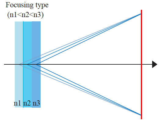
Figure 28: Schematic view of a proximity-focusing RICH with an inhomogeneous aerogel radiator in the focusing configuration. Cherenkov photons from the different radiator layers overlap, thus minimising the error in the angular resolution due to the uncertainly in the emission point [106].

5.6.1 Proximity-focusing aerogel RICH

The drawback of the proximity-focusing RICH technology is that for thicker radiators (needed to increase the number of photons) the emission point uncertainty ($\sigma_{EP}$ in Eq. 25) leads to a degradation of the single photon resolution. This limitation can be overcome by using a radiator made from several layers of aerogel with refractive indices gradually increasing, as is shown in Fig. 28. The corresponding Cherenkov rings are overlapping on the photon detector, which leads to an optimised angular resolution. Such a proximity-focusing RICH with inhomogeneous aerogel radiator is proposed for the endcap region of the upgraded Belle spectrometer [107, 108].

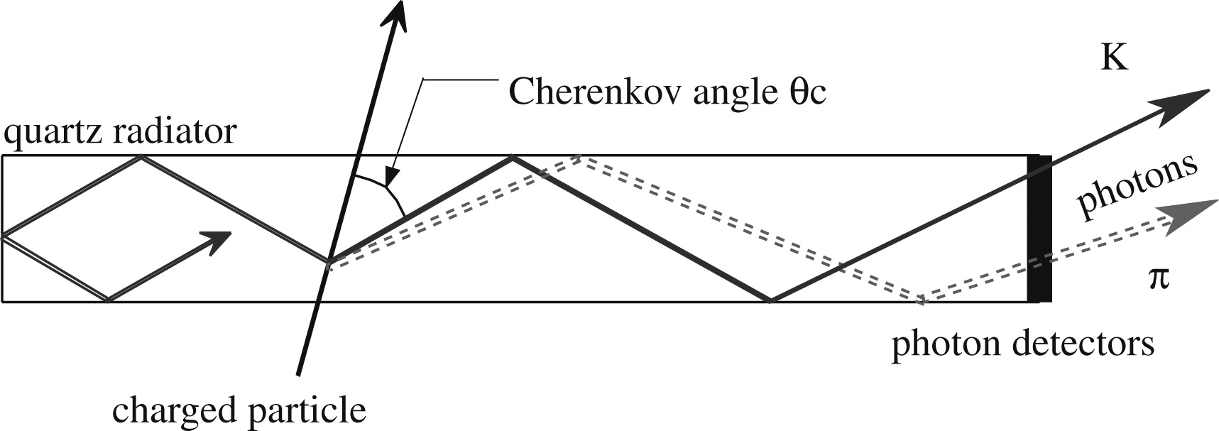
Figure 29: Schematic side view of a TOP counter [109]. Cherenkov photons are guided to the photon detector by total internal reflections. The difference in the propagation time for two particle types (here kaons and pions) is due to the emission angle of the Cherenkov radiation and can be used to enhance PID information.

5.6.2 Time-of-propagation counters

For the barrel region of the upgraded Belle spectrometer, a Time-of-propagation (TOP) counter is being studied [109, 110]. Here the two dimensional information of a Cherenkov ring image is represented by the time-of-arrival and impact position of the photons at the quartz bar exit window of a DIRC (see Fig.29). The construction is more compact than a DIRC, since the large expansion volume is not needed. A similar concept combining TOF and RICH techniques, named TORCH, was proposed for the LHCb upgrade as a possible solution for the identification of low momentum hadrons ($p<10$ GeV/c) [111]. It uses a large quartz plate to produce Cherenkov light and identifies the particles by measuring the photon arrival times.

6 PID in space

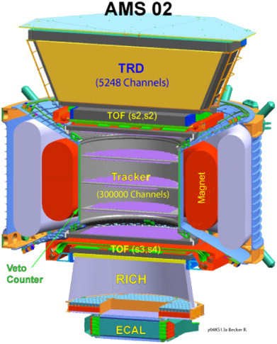
Figure 30: Schematic view of the AMS 02 spectrometer [112].

Non-accelerator experiments have become increasingly important in particle physics. An impressive example of a space-based experiment using a number of familiar PID techniques is the Alpha Magnetic Spectrometer (AMS 02 [112], see Fig. 30). The purposes of the experiment are to search for cosmic antimatter and dark matter and to study the composition and energy spectrum of the primary cosmic rays. The AMS 02 is set for installation on the International Space Station (ISS). It will be transported in the cargo bay of the space shuttle on its final mission, scheduled for 2011. The experiment will be attached to the outside of the space station and gather data that will be sent to a ground station for analysis.

The AMS 02 experiment is a state-of-the-art particle physics detector in space. The initial design included a superconducting magnet (0.9 T), which was however recently replaced by a permanent magnet (0.14 T) which allows the experiment to remain operational for the entire lifetime of the ISS (up to 18 years). The setup further includes a high-precision, double sided silicon strip detector and 4 dedicated PID devices: a TRD for electron ID (straw tubes filled with a mixture of Xe and CO₂ and fleece radiators), a proximity-focusing RICH with an aerogel radiator ($n=1.03$) for determination of the particle velocities and charges, a TOF detector (four planes of plastic scintillators) providing velocity determination and a fast trigger, and a sampling EM calorimeter (lead absorber plates and scintillating fibres). The whole system provides identification of particles and isotopes up to iron.

7 Summary and outlook

Particle identification (PID) is an important ingredient to particle physics experiments. Short-lived particles are reconstructed from their decay vertex and/or decay products. Some long-lived particles (leptons and photons) can be identified from the signatures they leave in the different layers of a typical experiment. Distinguishing the different long-lived charged hadrons (pions, kaons and protons) is more challenging, but often their identification is crucial, e.g. for precision measurements of rare processes with high statistics. Usually dedicated detectors are required for the task, which are based on the determination of the particle’s mass by simultaneous measurements of momentum $p$ and velocity $\beta=v/c$. The velocity is obtained by one of four techniques: measurement of the energy deposited through ionization, measurement of the time-of-flight, imaging of Cherenkov radiation or detection of transition radiation (transition radiation is not covered by this review). An illustrative comparison of the methods is shown in Fig. 5. The Cherenkov imaging method is the most flexible, as it allows to tune the response of the detector by varying the refractive index (and the length of the radiator), and makes accessible also very high momenta ($>$100 GeV/c). The Cherenkov and time-of-flight techniques can be used to close the gap in momentum in the MIP region, where PID by ionization measurements is not possible. All techniques are very well understood, with detectors being of the second, third or fourth generation, but the use and sophistication is still increasing as new generation detectors are built.

At the LHC, PID is one of the main challenges. Different concepts are followed: the two specialised experiments, ALICE for heavy-ion collisions and LHCb for B physics, make use of specific techniques adapted to their physics program. In both cases PID at low transverse momentum (but high total momentum in the case of LHCb) is important. ALICE actually uses all existing PID techniques. The general purpose detectors on the other hand, ATLAS and CMS, follow the traditional setup of a particle physics experiment: a tracking system, EM and hadron calorimeters and a muon system arranged in layers, with large acceptance for the identification of charged hadrons, photons and leptons. For their physics program, the challenges for precision calorimetry and precision muon detection are extremely high. Here the two experiments are actually following complementary approaches, but it can be expected that they are very competitive. All four experiments are very well advanced with the detector calibration. They have started to record data as the LHC began delivering p–p collisions in the year 2009. In the course of the year 2010, the increasing luminosity allowed real stress tests of the systems. At the end of that year also the first heavy-ion collisions were recorded by ALICE, ATLAS and CMS.

References

- [1] L. Evans et al. (Editors), LHC machine, JINST 3, S08001 (2008).
- [2] A. Andronic et al., Transition radiation detectors, this issue.
- [3] C. Mironov, Studying nuclear matter created in p+p, d+Au and Au+Au collisions using charged kaons, J. Phys.: Conf. Ser. 50 (2006) 311-314.
- [4] B. Brown et al., Electromagnetic calorimeters, this issue.
- [5] N. Akchurin et al., Hadron calorimetry, this issue.
- [6] A. Sharma et al., Muon detectors, this issue.
- [7] F. Hartmann, Vertex tracking detectors, this issue.
- [8] J. Podolanski et al., III. Analysis of V-events, Phil. Mag. 7 Vol. 45 (1954) 13-30.
- [9] W. Hulsbergen, Running status and first results from LHCb, Proceedings for the Rencontres de Moriond (2010 Electroweak Interactions and Unified Theories session).
- [10] The ATLAS Collaboration, G. Aad et al., The ATLAS Experiment at the CERN Large Hadron Collider, JINST 3, S08003 (2008).
- [11] The CMS Collaboration, S. Chatrchyan et al., The CMS experiment at the CERN LHC, JINST 3, S08004 (2008).
- [12] A. Bodek, Performance of a prototype CMS hadron barrel calorimeter in a test beam, IEEE Trans. Nucl. Sci. 46 (1999).
- [13] The ALICE Collaboration, K. Aamodt et al., The ALICE experiment at the CERN LHC, JINST 3, S08002 (2008).
- [14] ALICE Collaboration, A Large Ion Collider Experiment - Technical Proposal, CERN/LHCC-95-71.
- [15] F. Carminati et al., ALICE: physics performance report, volume I, J. Phys. G 30 (2004) 1517-1763.
- [16] B. Alessandro et al., ALICE: physics performance report, volume II, J. Phys. G 32 (2006) 1295-2040.
- [17] The ALICE collaboration, K. Aamodt et al., Charged-particle multiplicity density at mid-rapidity in central Pb-Pb collisions at TeV; arXiv:1011.3916v1 [nucl-ex].
- [18] The LHCb Collaboration, A. Augusto Alves Jr. et al., The LHCb Detector at the LHC, JINST 3, S08005 (2008).
- [19] F. Sauli, GEM: A new concept for electron amplification in gas detectors, Nucl. Instr. Meth. A 386 (1997) 531-534.
- [20] W. Blum et al., Particle Detection with Drift Chambers, 2nd ed., Springer Verlag, 2008.
- [21] H. Spieler, Semiconductor Detector Systems, Oxford University Press, 2005.
- [22] F. M. Penning, Über Ionisation durch metastabile Atome, Die Naturwissenschaften 15 (1927) 818-818.
- [23] C. Amsler et al. (Particle Data Group), The review of particle physics, Physics Letters B667 (2008) 1.
- [24] H. Bethe, Zur Theorie des Durchgangs schneller Korpuskularstrahlen durch Materie, Ann. Phys. 5 (1930) 325-400.
- [25] H. Bethe, Bremsformel für Elektronen relativistischer Geschwindigkeit, Z. Phys. 76 (1932) 293-299.
- [26] E. Fermi, The ionization loss of energy in gases and in condensed materials, Phys. Rev. 57 (1949) 485-493.
- [27] L. D. Landau, On the energy loss of fast particles by ionization, J. Phys. USSR 8 (1944) 201-205.
- [28] H. Bichsel, A method to improve tracking and particle identification in TPCs and silicon detectors, Nucl. Instr. and Meth. A 562 (2006) 154-197.
- [29] ALICE Collaboration, TPC Technical Design Report, CERN/LHCC 2000–001.
- [30] J. Alme et al., The ALICE TPC, a large 3-dimensional tracking device with fast readout for ultra-high multiplicity events, Nucl. Instr. and Meth. A 622 (2010) 316-367; arXiv:1001.1950v1 [physics.ins-det].
- [31] A. H. Walenta et al., Measurement of the ionization loss in the region of relativistic rise for noble and molecular gases, Nucl. Instr. and Meth. 161 (1979) 45-58.
- [32] E. Nappi, Advances in Charged Particle Identification Techniques, Proceedings of the 12th Vienna Conference on Instrumentation, Nucl. Instr. Meth. A 628 (2011) 1-8.
- [33] O. Ullaland, Update in particle identification, Nucl. Phys. B (Proc. Suppl.) 125 (2003) 90-99.
- [34] Y. Giomataris et al., MICROMEGAS: a high-granularity position-sensitive gaseous detector for high particle-flux environments, Nucl. Instr. Meth A 376 (1996) 29-35.
- [35] P. Schade et al., A large TPC prototype for a linear collider detector, Proceedings of the 12th Vienna Conference on Instrumentation, Nucl. Instr. Meth. A 628 (2011) 128-132.
- [36] M. Campbell et al., Detection of single electrons by means of a Micromegas-covered MediPix2 pixel CMOS readout circuit, Nucl. Instr. Meth. A 540 (2005) 295-304.
- [37] X. Llopart et al., Timepix, a 65k programmable pixel readout chip for arrival time, energy and/or photon counting measurements, Nucl. Instr. Meth. A 581 (2007) 485-494.
- [38] G. Tassielli et al., Cluster counting drift chamber as high precision tracker for ILC experiments, Nucl. Instr. Meth. A 617 (2010) 199-201.
- [39] E. Cerron Zeballos et al., A new type of Resistive Plate Chamber: The multigap RPC, Nucl. Instr. Meth. A 374 (1996), 132-136.
- [40] P. Fonte et al., A new high-resolution TOF technology, Nucl. Instr. and Meth. A 443 (2000) 201-204.
- [41] W. Riegler et al., Detector physics and simulation of Resistive Plate Chambers, Nucl. Instr. Meth. A 500 (2003) 144-162.
- [42] C. Lippmann et al., Space charge effects in Resistive Plate Chambers, Nucl. Instr. Meth. A 517 (2004) 54-76.
- [43] C. Lippmann et al., Rate effects in Resistive Plate Chambers, Nucl. Phys. B (Proc. Suppl.) 158 (2006) 127-130.
- [44] G. Aielli, Saturated logistic avalanche model, Nucl. Instr. Meth. A 508 (2003) 6-13, Proceedings of the 6th International Workshop on Resistive Plate Chambers and Related Detectors.
- [45] M. Abrescia et al., Progresses in the simulation of resistive plate chambers in avalanche mode, Nucl. Phys. B Proc. Suppl. 78, (1999) 459-464.
- [46] A. Mangiarotti et al., Exactly solvable model for the time response function of RPCs, Nucl. Instr. Meth. A 533 (2004) 16-21.
- [47] A. Mangiarotti et al., On the deterministic and stochastic solutions of Space Charge models and their impact on high resolution timing, Nucl. Phys. B Proc. Suppl. 158 (2006) 118-122, Proceedings of the 8th International Workshop on Resistive Plate Chambers and Related Detectors.
- [48] A. Blanco et al., Resistive plate chambers for time-of-flight measurements, Nucl. Instr. Meth. A 513 (2003) 8-12.
- [49] S. Afanasiev et al., The NA49 large acceptance hadron detector, Nucl. Instr. Meth. A 430 (1999) 210-244.
- [50] M. Shao et al., Extensive particle identification with TPC and TOF at the STAR experiment, Nucl. Instr. Meth. A 558 (2006) 419-429.
- [51] ALICE Collaboration, Addendum to TOF Technical Design Report, CERN/LHCC 2002-016.
- [52] G. Grancagnolo et al. (Editors), Resistive Plate Chambers 1999, Proceedings of the 5th International Workshop on Resistive Plate Chambers and Related Detectors, Nucl. Instr. Meth. A 456 (2000) 1.
- [53] P. Fonte et al. (Editors), Resistive Plate Chambers 2001, Proceedings of the 6th International Workshop on Resistive Plate Chambers and Related Detectors, Nucl. Instr. Meth. A 508 (2003) 1.
- [54] P. Dupieux et al. (Editors), Resistive Plate Chambers 2003, Proceedings of the 7th International Workshop on Resistive Plate Chambers and Related Detectors, Nucl. Instr. Meth. A 533 (2004) 1.
- [55] S. Park et al. (Editors), Resistive Plate Chambers 2005, Proceedings of the 8th International Workshop on Resistive Plate Chambers and Related Detectors, Nucl. Phys. B (Proc. Suppl.) 158 (2006) 1.
- [56] W. Barletta et al. (Editors), Resistive Plate Chambers 2007, Proceedings of the 9th International Workshop on Resistive Plate Chambers and Related Detectors, Nucl. Instr. Meth. A 602 (2009) 1.
- [57] Resistive Plate Chambers 2010, Proceedings of the 10th International Workshop on Resistive Plate Chambers and Related Detectors, to be published in Nucl. Instr. Meth. A.
- [58] W. Llope et al., The large-area time-of-flight upgrade for STAR, Nucl. Instr. Meth B 241 (2005) 306-310.
- [59] M. Shao et al., Extensive particle identification with TPC and TOF at the STAR experiment, Nucl. Instr. Meth. A 558 (2006) 419-429.
- [60] L. Ruan et al., Perspectives of a mid-rapidity dimuon program at the RHIC: a novel and compact muon telescope detector, J. Phys. G: Nucl. Part. Phys. 36 (2009) 095001 (15pp).
- [61] A. Schüttauf, Multi-strip MRPCs for FOPI, Nucl. Instr. Meth. A 602 (2009) 679-681.
- [62] D. Belver, The HADES RPC inner TOF wall, Nucl. Instr. Meth. A 602 (2009) 687-690.
- [63] J. Heuser, The Compressed Baryonic Matter Experiment at FAIR: Progress with feasibility studies and detector developments, Nucl. Phys. A 830 (2009) 563c-566c.
- [64] A. Akindinov, RPC with low-resistive phosphate glass electrodes as a candidate for the CBM TOF, Nucl. Instr. Meth. A 572 (2007) 676-681.
- [65] V. Ammosov, Performance of RPC with low-resistive silicate glass electrodes exposed to an intense continuous electron beam, Nucl. Instr. Meth. A 576 (2007) 331-336.
- [66] L. Lopes et al., Ceramic high-rate timing RPCs, Nuclear Physics B (Proc. Suppl.) 158 (2006) 66–70.
- [67] L. Naumann, Ceramics high rate Timing RPC, Proceedings of the 12th Vienna Conference on Instrumentation, Nucl. Instr. Meth. A 628 (2011) 138-141.
- [68] S. Korpar et al., Proximity focusing RICH with TOF capabilities, Nucl. Instr. Meth. A 572 (2007) 432-433.
- [69] K. Inami et al., A 5-ps TOF-counter with an MCP-PMT, Nucl. Instr. Meth. A 560 (2006) 303-308.
- [70] J. Va’vra et al., A high-resolution TOF detector: a possible way to compete with a RICH detector, Nucl. Instr. Meth. A 595 (2008) 270-273.
- [71] A. Roberts, A new type of C̆erenkov detector for the accurate measurement of the particle velocity and direction, Nucl. Instr. Meth. 9 (1960) 55-66.
- [72] J. Seguinot et al., Photo ionization and Cherenkov ring imaging, Nucl. Instr. Meth. 142 (1977) 377-391.
- [73] G. J. Barber et al., Glass-coated beryllium mirrors for the LHCb RICH1 detector, Nucl. Instr. Meth. A 570 (2007) 565-572 .
- [74] G. J. Barber et al., Development of lightweight carbon-fiber mirrors for the RICH 1 detector of LHCb, Nucl. Instr. Meth. A 593 (2008) 620-633.
- [75] T. Ypsilantis et al., Theory of ring imaging Cherenkov counters, Nucl. Instr. Meth. A 343 (1994) 30-51.
- [76] ALICE collaboration, ALICE high-momentum particle identification: Technical Design Report, CERN-LHCC-98-019.
- [77] E. Schyns, Status of large area CsI photocathode developments, Nucl. Instr. Meth A 494 (2002) 441-446.
- [78] A. Di Mauro et al., Study of the quantum efficiency of CsI photo-cathodes exposed to oxygen and water vapour, Nucl. Instr. Meth A 461 (2001) 584-586.
- [79] P. Martinengo et al., The ALICE high momentum particle identification system: An overview after the first Large Hadron Collider run, Proceedings of the seventh International Workshop on Ring Imaging Cherenkov detectors, to be published in Nucl. Instr. Meth. A.
- [80] A. Agocs et al., Very High Momentum Particle IDentification in ALICE at the LHC, Nucl. Instr. Meth. A 617 (2010) 424-429.
- [81] LHCb collaboration, LHCb RICH Technical Design Report, CERN/LHCC/2000-027.
- [82] LHCb collaboration, The re-optimized LHCb Detector Design and Performance, CERN/LHCC/2003-030.
- [83] P. Carlson, Aerogel Cherenkov counters: construction principles and applications, Nucl. Instr. Meth. A 248 (1986) 110-117.
- [84] M. Tabata et al., Development of transparent silica aerogel over a wide range of densities, Nucl. Instr. Meth. A 623 (2010) 339-341.
- [85] M. Moritz et al., Performance study of new pixel Hybrid Photon Detector prototypes for the LHCb RICH counters, IEEE Trans. Nucl. Sc. 51 (2004) 1060-1066.
- [86] C. Blanks, RICH alignment at LHCb with collision data, Proceedings of the seventh International Workshop on Ring Imaging Cherenkov detectors, to be published in Nucl. Instru. Meth. A.
- [87] E. Nappi et al. (Editors), Proceedings of first Workshop on Ring Imaging Cherenkov Detectors, Nucl. Instr. Meth. A 343 (1994) 1.
- [88] T. Ekelof (Editor), Proceedings of the Second International Workshop on Ring Imaging Cherenkov Detectors, Nucl. Instr. Meth. A 371 (1996) 1.
- [89] A. Breskin et al. (Editors), Proceedings of the Third International Workshop on Ring Imaging Cherenkov Detectors, Nucl. Instr. Meth. A 433 (1999) 1.
- [90] T. Ypsilantis et al. (Editors), Experimental Techniques of Cherenkov Light Imaging. Proceedings of the Fourth International Workshop on Ring Imaging Cherenkov Detectors, Nucl. Instr. Meth. A 502 (2003) 1.
- [91] J. Engelfried et al. (Editors), Proceedings of the fifth International Workshop on Ring Imaging Detectors, Nucl. Instr. Meth. A 553 (2005) 1.
- [92] A. Bressanet al. (Editors), RICH 2007 - Proceedings of the Sixth International Workshop on Ring Imaging Cherenkov Detectors, Nucl. Instr. Meth. A 595 (2008) 1.
- [93] Proceedings of the seventh International Workshop on Ring Imaging Cherenkov detectors, to be published in Nucl. Instr. Meth. A.
- [94] T. Ekelöf, The use and development of ring-imaging Cherenkov counters, CERN-PPE/91-23 (1991).
- [95] R. Bouclier et al., Progress in Cherenkov ring imaging: Part 1. Detection and localization of photons with the multistep proportional chamber, Nucl. Instr. Meth. 205 (1983) 403-423.
- [96] I. Ariño et al., The HERA-B Ring Imaging Cherenkov counter, Nucl. Instr. Meth. A 516 (2004) 445-461, [hep-ex/0303012].
- [97] P. Abbon et al., The fast photon detection system of COMPASS RICH-1, Nucl. Instr. Meth. A 581 (2007) 419-422.
- [98] T. Sumiyoshi et al., Silica aerogel Cherenkov counter for the KEK B-factory experiment, Nucl. Instr. Meth. A 433 (1999) 385-391.
- [99] M. Artuso et al., The CLEO RICH detector, Nucl. Instr. Meth. A 554 (2005) 147-194.
- [100] HADES collaboration, K. Zeitelhack et al., The HADES RICH detector, Nucl. Instr. Meth. A 433 (1999) 201-206.
- [101] A. Milov et al., Construction and expected performance of the hadron blind detector for the PHENIX experiment at RHIC, J. Phys. G 34 (2007) S701-S704.
- [102] BABAR-DIRC collaboration, J. Schwiening et al., Performance of the BABAR-DIRC, Nucl. Instr. Meth. A 553 (2005) 317-322.
- [103] C. Parkes, The LHCb upgrade, J. Phys.: Conf. Ser. 110 (2008) 092021 (3pp).
- [104] T. Iijima, Status and perspectives of vacuum-based photon detectors, Proceedings of the seventh International Workshop on Ring Imaging Cherenkov detectors, to be published in Nucl. Instr. Meth. A.
- [105] S. Korpar, Status and perspectives of solid state photon detectors, Proceedings of the seventh International Workshop on Ring Imaging Cherenkov detectors, to be published in Nucl. Instr. Meth. A.
- [106] S. Nishida et al., Studies of a proximity focusing aerogel RICH for the Belle upgrade, IEEE Nuclear Science Symposium Conference Record, Vol. 3 (2004) 1951-1955.
- [107] T. Iijima et al., A novel type of proximity focusing RICH counter with multiple refractive index aerogel radiator, Nucl. Instr. Meth. A 548 (2005) 383-390.
- [108] A. Danilyuk et al., Focusing aerogel RICH (FARICH), Nucl. Instr. Meth. 553 (2005) 70-75.
- [109] M. Akatsu et al., Time-Of-Propagation Cherenkov counter for particle identification, Nucl. Instr. Meth. A 440 (2000) 124-135.
- [110] K. Inami, Development of a TOP counter for the super B factory, Nucl. Instr. Meth. A 595 (2008) 96-99.
- [111] M. J. Charles et al., TORCH: Time of flight identification with Cherenkov radiation, Nucl. Instr. Meth. A; arXiv:1009.3793v1 [physics.ins-det].
- [112] V. Bindi, The alpha magnetic spectrometer AMS-02: Soon in space, Nucl. Instr. Meth. A 617 (2010) 462-463.