Unveiling the Nature of Three Dimensional Orbital Ordering Transitions:
The Case of $e_{g}$ and $t_{2g}$ Models on the Cubic Lattice

Abstract

We perform large scale finite-temperature Monte Carlo simulations of the classical $e_{g}$ and $t_{2g}$ orbital models on the simple cubic lattice in three dimensions. The $e_{g}$ model displays a continuous phase transition to an orbitally ordered phase. While the correlation length exponent $\nu\approx 0.66(1)$ is close to the 3D XY value, the exponent $\eta\approx 0.15(1)$ differs substantially from O(N) values. At $T_{c}$ a $U(1)$ symmetry emerges, which persists for $T<T_{c}$ below a crossover length scaling as $\Lambda\sim\xi^{a}$, with an unusually small $a\approx 1.3$. Finally, for the $t_{2g}$ model we find a first order transition into a low-temperature lattice-nematic phase without orbital order.

Orbital-only models emerged recently as prototype systems enabling the understanding of relevant aspects of the collective dynamics of orbital degrees of freedom vandenBrink_NJP . In a different context, orbital-like models are attracting considerable theoretical interest due to their ability to sustain topologically ordered phases with possibly anyonic excitations, as exemplified by the Kitaev honeycomb model kitaev-model . In a similar spirit the orbital compass model kugel82 can serve as a basic model to understand topologically protected Josephson junction qubits doucot:024505 , which have recently been realized experimentally gladchenko-2008 .

A variety of properties have already been uncovered for orbital-only models, but most of these are restricted to ground state or low-temperature properties. Much less is known about finite-temperature properties and in particular the nature of thermal phase transitions. Those might display new critical phenomena, as a common feature of all these systems is a manifest coupling between order parameter space and real space, which distinguishes them from the well studied O(N) (such as Ising, XY and Heisenberg) models vicarireview .

In this Letter, we present a comprehensive Monte Carlo (MC) investigation of the nature of the finite-temperature phase transitions in two popular orbital-only models on the three-dimensional (3D) cubic lattice: the $e_{g}$ and the $t_{2g}$ models vandenBrink_NJP . We study here the classical versions because the corresponding quantum models have a sign problem precluding Quantum Monte Carlo approaches, and because in Ginzburg-Landau theory one typically expects quantum and classical versions of a same model to have the same critical properties, although exceptions are possible. The $e_{g}$ and the $t_{2g}$ models are also often called the $120^{\circ}$ and compass models, respectively. While the thermal phase transition in the two-dimensional (2D) compass model has been the focus of recent studies mishra:207201 ; wenzelQCMPRB ; wenzelCM2010 and clarified to belong to the 2D Ising universality class, little is known about the $e_{g}$ and $t_{2g}$ models in 3D - although potentially of more direct relevance for the description of collective orbital phenomena vandenBrink_NJP . We start by discussing the $e_{g}$ model and its critical properties in some detail and turn then briefly to the $t_{2g}$ model towards the end of this paper.

The $e_{g}$ model —

The $e_{g}$ model (EgM) is defined by the Hamiltonian vandenBrink_NJP

$$\mathcal{H}_{e_{g}}=-\ J\sum_{i,\alpha}{\boldsymbol{\tau}}_{i}^{\alpha}{\boldsymbol{\tau}}_{i+\mathbf{e}_{\alpha}}^{\alpha},$$ (1)

where $\boldsymbol{\tau}_{i}$ is an auxiliary three component vector obtained by an embedding of the orbital degree of freedom $\mathbf{T}_{i}=(T^{z}_{i},T^{x}_{i})\in S^{1}$:

$${\boldsymbol{\tau}}_{i}=\begin{pmatrix}-1/2&\sqrt{3}/2\\ -1/2&-\sqrt{3}/2\\ 1&0\end{pmatrix}\mathbf{T}_{i}.$$ (2)

The $\mathbf{e}_{\alpha}$ denote the positive unit vectors in the $\alpha\in\{x,y,z\}$ cartesian directions. Note that the coupling in $\boldsymbol{\tau}$-space depends on the spatial orientation of the bond. The coupling constant $J$ is set to one in the following, corresponding to ferromagnetic interactions. Note that results for antiferromagnetic interactions can be deduced from results using ferromagnetic couplings Rynbach .

The classical EgM (1) has a sub-extensive ground state degeneracy which is lifted at finite temperature by an order by disorder mechanism nussinov-2004-6 , leading to six discrete ordering directions $\mathbb{T}^{o}_{n}=\left(\cos[n\ 2\pi/6],\sin[n\ 2\pi/6]\right)$ with $n=0,\dots,5$. This analytical prediction has been verified using classical MC simulations tanaka:267204 ; Rynbach , and at higher temperatures a continuous phase transition to a disordered phase has been found. The prominent question of the universality class of the finite-temperature phase transition is however still open, both analytically and numerically. Comparing to related systems with a similar low-temperature phase, several different scenarios seem possible: i) a continuous transition in the universality class of the 3D XY model, as e.g. in the $Z_{6}$-perturbed XY models Jose_PRB ; Blankschtein_PRB ; Oshikawa_Zn ; Louclock , ii) distinct universality classes, as reported in classical dimer models on the cubic lattice FAlet-dimer ; CharrierAlet2010 or iii) a first order transition, as in a six-state ferromagnetic Potts model in 3D, or a Heisenberg ferromagnet with a specific cubic anisotropy vicarireview . In the following, we shall resolve this fundamental question and answer which scenario is realized for the $e_{g}$ and $t_{2g}$ models.

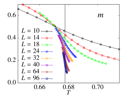
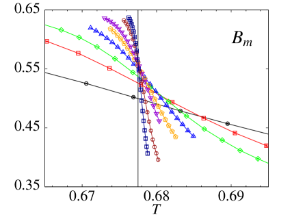
Figure 1: (Color online). $e_{g}$ model: The order parameter $m$ (left plot) and the associated Binder cumulant $B_{m}$ (right plot) as a function of temperature $T$ for different linear system sizes $L$. The vertical line indicates the location of the critical temperature.

Simulation technique and observables —

We consider the classical Hamiltonian (1) on a simple cubic lattice of side length $L$ and volume $N=L^{3}$ and perform state-of-the-art MC simulations along the lines of Refs. wenzelQCMPRB ; wenzelCM2010 . Simulations were performed for lattice sizes $L=8,\dots,96$. To obtain the reported accuracy, we collected $10^{6}$ and more independent MC measurements per data point. MC runs using periodic boundary conditions (PBC) show clear signals of a transition to an ordered phase in accordance with Ref. Rynbach . However, as further demonstrated below, we find that there are severe finite-size corrections using PBC. Fortunately, we possess an efficient tool to substantially reduce the strong finite-size effects of PBC by employing screw-periodic boundary conditions (SBC), as shown recently for the 2D compass model in Ref. wenzelCM2010 . Here, we shift the cube $L/2$ steps in the $x$-direction when leaving the $zy$-face (plus cyclic permutations), which we empirically find to minimize finite-size effects WenzelEGlong . A natural order parameter to detect orbital ordering in the following is:

$$m=(1/N)\sqrt{(\sum_{i}T^{z}_{i})^{2}+(\sum_{i}T^{x}_{i})^{2}},$$ (3)

while the complementary quantity $D$ indicates a directional ordering of the bond energies:

$$D=(1/N)\sqrt{\left(E_{x}-E_{y}\right)^{2}+\left(E_{y}-E_{z}\right)^{2}+\left(E_{z}-E_{x}\right)^{2}},$$ (4)

which was previously studied in the compass model mishra:207201 ; wenzelQCMPRB ; wenzelCM2010 . Here, $E_{x|y|z}$ is the total bond-energy along the ${x|y|z}$-direction.

Critical exponents in the $e_{g}$ model —

We start by presenting numerical results for the EgM (1) with SBC by displaying in Fig. 1 the data for the magnetization $m$ and the Binder parameter $B_{m}=1-\langle m^{4}\rangle/3\langle m^{2}\rangle^{2}$ as a function of temperature. Both observables indicate a continuous phase transition at about $T_{c}\approx 0.677$, in agreement with earlier PBC estimates tanaka:267204 ; Rynbach . At $T_{c}$ we expect $B_{m}(L)$ to possess only corrections to scaling $B_{m}(L)=B_{m}^{\star}+cL^{-\omega}$ with $\omega$ being the correction exponent. We find our best estimate for $T_{c}=0.6775(1)$ and an effective $\omega\approx 1.4$ with a large constant $c$.

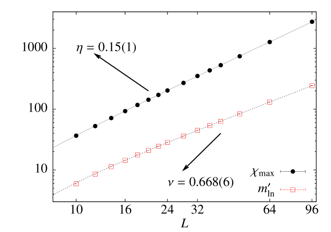
Figure 2: (Color online). $e_{g}$ model: Plot of $\chi_{\max}$ and $m^{\prime}_{\ln}$ versus $L$ in a double logarithmic scale. Estimates for $\nu$ and $\eta$ where obtained from a finite-size study using Eq. (5), taking into account corrections to scaling. The lines are the corresponding fit curves.

We now perform a finite-size scaling study to obtain the critical exponents. Here, we concentrate primarily on the correlation length exponent $\nu$ describing the divergence of the correlation length close to the critical point $\xi\sim\left|T-T_{c}\right|^{-\nu}$, as well as the exponent $\eta$ governing the decay of the spin-spin correlation function $G(r)\sim r^{-d+2-\eta}$ at the critical point. We determine these exponents using the derivative of the logarithm of the order parameter $m^{\prime}_{\ln}=\max\{(\mathrm{d}\ln m/\mathrm{d}\beta)\}$ and the maximum of the susceptibility $\chi_{\max}=\max\{N\left(\langle m^{2}\rangle-\langle m\rangle^{2}\right)\}$ which are known to scale with system size $L$ as: JankeMCGreifswald

$$m^{\prime}_{\ln}\sim L^{1/\nu}(1+c_{m^{\prime}}L^{-\omega}),\,\,\chi_{\max}\sim L^{2-\eta}(1+c_{\chi}L^{-\omega}).$$ (5)

Using the effective correction exponent $\omega$ obtained above based on the Binder cumulant, the data fits very well to Eq. (5) yielding our estimate $\nu=0.668(6)$ for the correlation length exponent, see Fig. 2. This value for $\nu$ would be roughly consistent with the universality class of the 3D XY universality) with $\nu_{\mathrm{XY}}=0.671$ CampostriniXY . However, an analogous analysis of the order parameter correlations at criticality - from which we obtain $\eta=0.15(1)$ Footnote_eta - provides strong evidence for a universality class distinct from the 3D XY class, which would yield a substantially smaller $\eta_{\mathrm{XY}}\approx 0.038$ vicarireview ; CampostriniXY . Finally, an analysis of the exponent $\alpha$ gives $\alpha\approx 0$ in agreement with the usual hyper-scaling relation.

Critical exponents in the $e_{g}$-clock model—

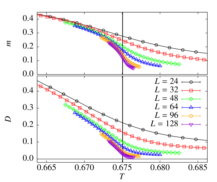
Figure 3: (Color online). $e_{g}$-clock model: Orbital order parameter $m(T)$ (upper panel) and directional order parameter $D(T)$ (lower panel) for different linear system sizes $L$. Note that both order parameters become finite below a common $T_{c}$ (indicated by the vertical line).

To investigate whether the continuous nature of the microscopic degrees of freedom $\mathbf{T}$ has an impact on the critical properties, we now consider a discrete version of Hamiltonian (1) – one in which the vectors $\mathbf{T}$ can only point along the six $\mathbb{T}^{o}_{n}$ ordering directions introduced above:

$$\mathcal{H}_{e_{g}}^{\circledast}=-\ J\sum_{i,\alpha}E^{\alpha}(n_{i},n_{i+\mathbf{e}_{\alpha}})\,.$$ (6)

Here, $E^{\alpha}(n_{i},n_{j})$ is the bond energy matrix along the bond direction $\alpha$ and $n=0,\ldots,5$ denote the six discrete onsite states. The similarity of our model to the 6-state ($Z_{6}$) clock model $\mathcal{H}_{Z_{6}}=-J\sum_{\langle i,j\rangle}\mathbb{T}^{o}_{n_{i}}\cdot\mathbb{T}^{o}_{n_{j}}$ Potts1952 , suggests to term $\mathcal{H}_{e_{g}}^{\circledast}$ the $e_{g}$-clock model (EgCLM). Its discrete nature allows to study larger systems of up to $L=128$. In addition, we analyze the directional order parameter $D$ as introduced in Eq. (4). In an orbitally ordered state characterized by a finite $m$, $D$ is also finite, however the converse is not true. An illustrative example is given by the 2D compass model, where a gauge-like freedom forbids orbital ordering altogether nussinovpip , while $D$ orders at finite temperature mishra:207201 ; wenzelQCMPRB ; wenzelCM2010 .

In Fig. 3 we present data for $m(T)$ (upper panel) and $D(T)$ (lower panel) for different system sizes. Both $m$ and $D$ appear to set in at about the same temperature. In order to confirm the simultaneous onset we have determined the respective Binder parameters $B_{m}$ and $B_{D}$ (not shown), indicating that both transitions take place at a unique critical temperature $T_{c}=0.67505(3)$. This result rules out a scenario of a directionally ordered, orbital-disordered intermediate phase, and establishes a single transition from a high temperature disordered phase to a low temperature orbitally ordered phase.

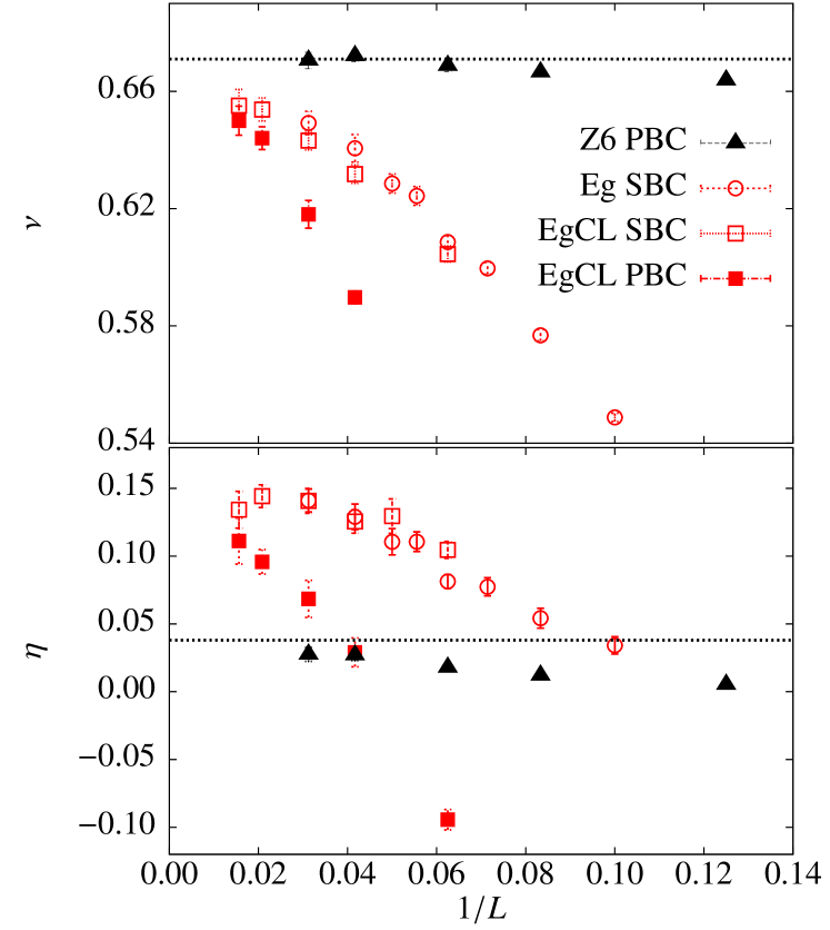
Figure 4: (Color online). Finite-size scaling of the running exponents $\nu_{L}$ and $\eta_{L}$ calculated from Eqs. (7) and (8) for several models and boundary conditions, see legend. Both the $e_{g}$ and the $e_{g}$-clock model display the same critical behavior, which is different from the 3D XY universality class (indicated by the dashed lines and similar data for the $Z_{6}$-clock model known to approach 3D XY universality Jose_PRB ).

Having demonstrated the simultaneity of the two ordering phenomena, we now perform a systematic study of the critical exponents in the EgCLM. Instead of fitting to Eq. (5), we study the finite-size behavior of (running) critical exponents obtained on system sizes $L$ and $2L$ via the relations

$$\nu{{}_{L}} =\ln(2)/\ln\left(m^{\prime}_{\ln}(2L)/m^{\prime}_{\ln}(L)\right),$$ (7)

$$\eta{{}_{L}} =2-\ln\left(\chi_{\max}(2L)/\chi_{\max}(L)\right)/\ln(2).$$ (8)

This allows to visualize finite-size effects directly and should give the true exponents for $L\to\infty$. In Fig. 4 we present results for $\nu_{L}$ (upper panel) and $\eta_{L}$ (lower panel). In both quantities strong finite-size corrections are evident for the EgM and EgCLM, but our results convincingly show that different boundary conditions (PBC/SBC) and both the EgM and the EgCLM converge to a single set of exponents: $\nu\approx 0.66$ and $\eta\approx 0.15$. These exponents - especially $\eta$ - are at variance with the corresponding values of the 3D XY universality class. For comparison, we include data for the $Z_{6}$-clock model in Fig. 4, which quickly converges to the 3D XY exponents expected for this model Jose_PRB . Note that a similar analysis based on the order parameter $D$ instead of $m$ leads to the same $\nu$ exponent, while the corresponding $\eta_{D}$ exponent is much larger $(\approx 1.4)$. This simply follows from the assumption that $D$ has no intrinsic critical behavior, because then $D$ is driven by $m$: $D\sim m^{2}$, resulting in an apparently different $\eta$ value.

Emergent U(1) symmetry —

In order to shed light on the possible emergence of a U(1) symmetry at the critical point and the associated behavior of the crossover length scale $\Lambda$ for $T<T_{c}$ (as discussed in the context of $Z_{q}$-perturbed XY models Jose_PRB ; Blankschtein_PRB ; Oshikawa_Zn ; Louclock ), we determine the 6-fold anisotropy $m_{6}$ of the orbital order $m$, based on order parameter histograms $P(r,\theta)$ Louclock :

$$m_{6}=\int_{0}^{1}dr\int_{0}^{2\pi}d\theta r^{2}P(r,\theta)\cos(6\theta).$$ (9)

An analysis for the EgCLM analogous to Ref. Louclock yields a scaling of the crossover length $\Lambda$ with the correlation length $\xi$ as $\Lambda\sim\xi^{a_{6}}$, with $a_{6}\approx 1.3$ [c.f. Fig. 5(a)]. In the case of a $Z_{6}$-perturbed 3D XY model we find $a_{6}^{XY}\approx 2.2$ (c.f. Fig. 5(b), compatible with Ref. Louclock ), almost a factor two larger than the value we obtain for the EgCLM.

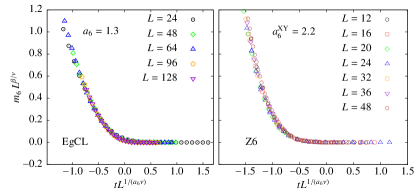
Figure 5: (Color online). Collapse analysis of $m_{6}$ [see Eq. (9)] for the $e_{g}$-clock model (left) and the $Z_{6}$-clock model (right), based on the scaling assumption $m_{6}\sim L^{-\beta/\nu}g(tL^{1/(a_{6}\nu)})$ (see Ref. Louclock ). Best collapse parameters $a_{6}$ are indicated in the plot and differ clearly for the two models.

Compass ($t_{2g}$) model —

Finally we report our results for the second orbital-only model of interest here, the $t_{2g}$ model in three dimensions vandenBrink_NJP , defined as:

$$\mathcal{H}_{t_{2g}}=-\ J\sum_{i,\mathbf{e}_{\alpha}}\mathbf{T}_{i}^{\alpha}\mathbf{T}_{i+\mathbf{e}_{\alpha}}^{\alpha},$$ (10)

where now the degree of freedom $\mathbf{T}=(T^{x},T^{y},T^{z})$ is a unit vector on the sphere $S^{2}$, and otherwise the notation follows Eq. (1). This model is also called 3D compass model and is a straightforward generalization of the 2D compass model studied e.g. in mishra:207201 ; wenzelQCMPRB ; wenzelCM2010 . An important difference of the $t_{2g}$ model compared to the $e_{g}$ model is that orbital order is ruled out due to the presence of gauge-like symmetries nussinovpip . Therefore, the order parameter $D$ [Eq. (4)] can exhibit a phase transition in the absence of orbital ordering. We have simulated the full classical $t_{2g}$ model using the same simulation technology as for the $e_{g}$ model, revealing a first order transition at $T_{c}\approx 0.098$ from a high-temperature disordered to a low-temperature lattice symmetry broken phase indicated by a finite value of $D$.

Recently the quantum $t_{2g}$ model has been studied using series expansions Oitmaa2010 , and the absence of a phase transition at finite temperature was conjectured. Our findings for the classical $t_{2g}$ model provide an alternative explanation as to why no (second order) finite-temperature transition was detected: due to the first order nature, the transition is intrinsically difficult to detect based on series expansions. A detailed analysis of the properties of the $t_{2g}$ model will be presented in a forthcoming publication WenzelEGlong .

Conclusions —

We have provided a detailed analysis of the critical properties of the finite-temperature ordering transitions in $e_{g}$ and $t_{2g}$ orbital-only models. While the $t_{2g}$ model exhibits a first order transition, the critical properties of the $e_{g}$ model point towards a distinct universality class, different from the standard classes we have encountered so far. Further theoretical work will be required to shed light on this observation, and to understand in more detail the peculiar effects of the coupling of real space and order parameter space vicarireview ; Nattermann1975 , which are at work in these models. Given the broad range of systems where models similar to the ones studied here could arise (orbital systems in solids vandenBrink_NJP ; Jackeli2009 , Josephson junction arrays gladchenko-2008 , and artificially engineered systems in optical lattices Duan2003 ), we are optimistic that the peculiar critical properties uncovered in the present work can be further explored experimentally.

- (1) J. van den Brink, New J. Phys. 6, 201 (2004).
- (2) A.Y. Kitaev, Ann. Phys. 321, 2 (2006).
- (3) K.I. Kugel and D.I. Khomskii, Sov. Phys. Usp. 25, 231 (1982).
- (4) B. Douçot et al., Phys. Rev. B 71, 024505 (2005).
- (5) S. Gladchenko et al., Nat. Phys. 5, 48 (2009).
- (6) A. Pelissetto and E. Vicari, Phys. Rep. 368, 549 (2002).
- (7) A. Mishra et al., Phys. Rev. Lett. 93, 207201 (2004).
- (8) S. Wenzel and W. Janke, Phys. Rev. B 78, 064402 (2008).
- (9) S. Wenzel, W. Janke, and A. M. Läuchli, Phys. Rev. E 81, 066702 (2010).
- (10) A. van Rynbach, S. Todo, and S. Trebst, Phys. Rev. Lett. 105, 146402 (2010).
- (11) Z. Nussinov et al., Europhys. Lett. 67, 990 (2004); M. Biskup, L. Chayes, and Z. Nussinov, Commun. Math. Phys. 255, 253 (2005).
- (12) T. Tanaka, M. Matsumoto, and S. Ishihara, Phys. Rev. Lett. 95, 267204 (2005).
- (13) J.V. José et al., Phys. Rev. B 16, 1217 (1977).
- (14) D. Blankschtein et al., Phys. Rev. B 29, 5250 (1984).
- (15) M. Oshikawa, Phys. Rev. B 61, 3430 (2000).
- (16) J. Lou, A.W. Sandvik, and L. Balents, Phys. Rev. Lett. 99, 207203 (2007).
- (17) F. Alet et al., Phys. Rev. Lett. 97, 030403 (2006).
- (18) D. Charrier and F. Alet, Phys. Rev. B 82, 014429 (2010).
- (19) S. Wenzel and A. M. Läuchli. unpublished (2011).
- (20) The slope of the Binder parameter gives consistent results but shows larger statistical fluctuations.
- (21) W. Janke, Lect. Notes Phys. 739, 79 (2008).
- (22) M. Campostrini et al., Phys. Rev. B 63, 214503 (2001).
- (23) A straight line fit for yields .
- (24) R. B. Potts, Proc. Camb. Philos. Soc. 48, 106 (1952).
- (25) Z. Nussinov and E. Fradkin, Phys. Rev. B 71, 195120 (2005).
- (26) J. Oitmaa and C.J. Hamer, Phys. Rev. B 83, 094437 (2011).
- (27) T. Nattermann and S. Trimper, J. Phys. A: Math. Gen. 8, 2000 (1975).
- (28) G. Jackeli and G. Khaliullin, Phys. Rev. Lett. 102, 017205 (2009); J. Chaloupka, G. Jackeli, and G. Khaliullin, Phys. Rev. Lett. 105, 027204 (2010).
- (29) L.-M. Duan, E. Demler, and M. D. Lukin, Phys. Rev. Lett. 91, 090402 (2003); A. Micheli, G.K. Brennen, and P. Zoller, Nat. Phys. 2, 341 (2006).