dot.

UDC 531

S. S. ZUB

Abstract. The stability of the orbital motion of two long cylindrical magnets interacting exclusively with magnetic forces is described. To carry out analytical studies a model of magnetically interacting symmetric tops [1] is used. The model was previously developed within the quasi-stationary approach for an electromagnetic field based on the general expression of the energy of interacting magnetic bodies [2]. A special role in the investigation of the stability of orbital motions is played by the so-called relative equilibria [3], i.e. the trajectories of the system dynamics which are at the same time one-parameter subgroups of the system invariance group. Nowadays their stability is normally investigated using two similar approaches – energy-momentum and energy-Casimir methods. The most suitable criterion for the system stability investigation was formulated in the theorem of [4]; this stability criterion successfully generalizes both the methods mentioned above and covers the Hamiltonian formalism based on Poisson structures [1]. The necessary and sufficient conditions for the circular orbit stability are derived from this theorem.

1. Introduction

The paper describes the new results on the research into the orbital motion stability of magnetically interacting bodies. It continues the cycle of papers devoted to the investigation of contact-free confinement of bodies by means of magnetic forces.

There are two different historical aspects of our problem, physical and mathematical.

The physical aspect is attributed to V.V. Kozoriz who was the first to come out in 1974 with a supposition about the possibility of stable dynamic states in the so-called ’’compact’’ magnetic configurations.

At that time an opinion about the global instability of electric and magnetic systems within the classical electrodynamics was widespread among physicists [5]. These ideas in statics were associated with Earnshaw’s theorem; in dynamics they are associated with the so-called ’’$1/r^{3}$ problem’’.

The supposition of V.V. Kozoriz seemed to be paradoxical and received no support in the scientific community; therefore he actually carried out his research on his own.

In his papers, among which monograph [6] is worthy of mentioning about, he gave a whole number of models and predicted the orbital motion stability for them.

Applying the physical idea about the nature of stability in such systems and analyzing the behaviour of the potential energy of the considered systems he gave a number of stability criteria for these systems.

However, the method he used for investigating the stability cannot be called rigorous. Now it is quite clear that the proposed orbit stability conditions are not sufficient.

Comparatively not long ago V.V. Kozoriz and his co-authors made numerical modelling of the system of two long cylindrical magnets using a PC-cluster from the Institute of Cybernetics; they managed to discover a number of stable orbits [7]. However, they didn’t produce any analytical proof of stability in this paper.

At the moment the hypothesis about the possibility of stable orbital motions in ’’compact’’ magnetic systems was made the suitable methods of analytical stability investigation were only at the initial stage of their development and were unknown to physicists for a long period of time.

This second, mathematical, aspect is associated with such names as B. Konstant, J.-M. Souriau, V. I. Arnold, A. A. Kirillov, and especially with J. E. Marsden. Marsden’s lectures given in the Royal Mathematical Society and published in a separate book [3] are completely devoted to the stability problem. For several decades his scientific school has been developing the theory of stability of Hamiltonian systems with symmetry and applying it in the research into fluid flow, stability of plasma, elastic bodies, in the general theory of relativity and the quantum field theory.

However, among the numerous results of these books and papers of his colleagues we could not discover any result which would be completely suitable for our system. This is due to the fact that the basic results on stability of Hamiltonian systems concern symplectic manifolds. The paper of J.-P. Ortega and T. S. Ratiu [4] is an exception; their theorem concerns an analytically more complicated case of Poisson structures. It is the theorem that we use in our paper.

2. Hamiltonian formalism based on Poisson structures

The Hamiltonian formalism based on Poisson structures (PS) [1] gives an algebraic coordinate-free representation of dynamics which is especially important when a system consists of rigid bodies.

In our case the Poisson manifold is the direct product of Euclidean spaces

$$P=R^{3}_{x}\times R^{3}_{p}\times R^{3}_{\mu}\times R^{3}_{m}\times R^{3}_{\nu}\times R^{3}_{n}.$$ (2.1)

Thus, the generatrices of our dynamic system will be $x_{i}$ as relative coordinates of two bodies; $p_{i}$ as pulse components of relative (orbital) motion; $m_{i}$, $n_{i}$ as components of angular momentums of the 1st and 2nd body, respectively; $\mu_{i}$, $\nu_{i}$ as components of unit vectors of symmetry axes for the 1st and 2nd body, respectively.

The nonzero Poisson brackets between the generatrices on $P$ are as follows,

$$\begin{cases}\{x_{i},p_{j}\}=\delta_{ij};\\ \{m_{i},\mu_{j}\}=\varepsilon_{ijk}\mu_{k};\quad{\ }\{m_{i},m_{j}\}=\varepsilon_{ijk}m_{k};\\ \{n_{i},\nu_{j}\}=\varepsilon_{ijk}\nu_{k};\quad\{n_{i},n_{j}\}=\varepsilon_{ijk}n_{k},\end{cases}$$ (2.2)

and the remaining influential Poisson brackets are equal to zero.

It can be easily checked that the Casimir functions of this Poisson structure will be

$$\begin{cases}\vec{\mu}{\ }^{2}=1,\quad\vec{\nu}{\ }^{2}=1;\\ (\vec{\mu}{\ },\vec{m})=M_{3}=const_{1},\quad(\vec{\nu}{\ },\vec{n})=N_{3}=const_{2}.\end{cases}$$

The Hamiltonian of the system can be written in the following form

$$h=T+U(r,c^{{}^{\prime}},c^{{}^{\prime\prime}},c^{{}^{\prime\prime\prime}}),$$ (2.3)

where

$$\begin{cases}r=|\vec{x}|;\quad\vec{e}=\vec{x}/r;\\ c^{{}^{\prime}}=(\vec{e},\vec{\mu});\\ c^{{}^{\prime\prime}}=(\vec{e},\vec{\nu});\\ c^{{}^{\prime\prime\prime}}=(\vec{\mu},\vec{\nu}).\end{cases}$$

This form of the potential energy $U$ describes a wide enough class of paired interactions of magnetic bodies such as rotationally symmetric permanent magnets, superconducting rings and solenoids, dipoles, and mixed systems [2].

3. Problem on stable orbital motion of two cylindrical magnets

We will use the constructive proof method to prove the existence of stable orbital systems interacting with magnetic forces. It means that we will demonstrate the possibility of stability on the example of a specific physical system of this type.

We will take two identical long cylinders as magnetic bodies. As it was shown earlier in our paper [1], the interaction of such bodies can be described by the Coulomb potential energy of four fictitious magnetic charges [8] concentrated on the extensions of the cylinders. Thus, the potential energy of the system takes the following form

$$U=\frac{\mu_{0}\kappa^{{}^{\prime}}\kappa^{{}^{\prime\prime}}}{4\pi}\sum_{\varepsilon^{{}^{\prime}},\varepsilon^{{}^{\prime\prime}}=\pm 1}\frac{\varepsilon^{{}^{\prime}}\varepsilon^{{}^{\prime\prime}}}{R_{\varepsilon^{{}^{\prime}}\varepsilon^{{}^{\prime\prime}}}},$$ (3.1)

where $R_{\varepsilon^{{}^{\prime}}\varepsilon^{{}^{\prime\prime}}}(r,c^{{}^{\prime}},c^{{}^{\prime\prime}},c^{{}^{\prime\prime\prime}})=\sqrt{r^{2}+l^{{}^{\prime}2}+l^{{}^{\prime\prime}2}+2r(\varepsilon^{{}^{\prime\prime}}l^{{}^{\prime\prime}}c^{{}^{\prime\prime}}-\varepsilon^{{}^{\prime}}l^{{}^{\prime}}c^{{}^{\prime}})-2\varepsilon^{{}^{\prime}}\varepsilon^{{}^{\prime\prime}}l^{{}^{\prime}}l^{{}^{\prime\prime}}c^{{}^{\prime\prime\prime}}}$; $l^{{}^{\prime}}$, $l^{{}^{\prime\prime}}$ are semilengths of the cylinders; $r$ is the distance between the centers of the cylinders; $\kappa^{{}^{\prime}}$, $\kappa^{{}^{\prime\prime}}$ are quantities of fictitious charges.

The potential energy in point (3.1) is a special case of the potential energy in (2.3).

Let us consider the problem in the center-of-mass system of the bodies [1].

The kinetic energy of the system will be formed by the kinetic energies of translational (orbital) motion of the bodies and their self-rotation kinetic energies:

$$T(p^{2},\vec{m}^{2},\vec{n}^{2})=\frac{1}{2m}p^{2}+\frac{\alpha}{2}\vec{m}^{2}+\frac{\beta}{2}\vec{n}^{2},$$

where $\vec{r}$, $\vec{p}$ are orbital coordinates and pulses; $\vec{m}$, $\vec{n}$ are angular momentums of the 1st and 2nd body, respectively; $m=\frac{m_{1}m_{2}}{m_{1}+m_{2}}$; $\alpha=\beta=\frac{1}{I_{\bot}}$ (if the principal moments of inertia of the body are equal to each other, $I_{1}=I_{2}=I_{\bot}$, the rigid body is termed a symmetric top).

Remark: If the consideration is limited to symmetric tops it is possible to use the uniform Cartesian frame, the components of physical vector quantities being suitable generatrices for the Poisson structure. In this case the Poisson brackets of dynamic vector variables can be considered, and the equations of motion can be written in a vector form [1].

The corresponding Hamiltonian equations of motion are as follows

$$\begin{cases}\dot{\vec{r}}=\frac{1}{m}\vec{p};\\ \dot{\vec{p}}=-{\partial}_{r}U\vec{e}-\frac{1}{r}({\partial}_{c^{{}^{\prime}}}UP_{\bot}^{e}(\vec{\mu})+{\partial}_{c^{{}^{\prime\prime}}}UP_{\bot}^{e}(\vec{\nu}));\\ \dot{\vec{\mu}}=\alpha(\vec{m}\times\vec{\mu});\\ \dot{\vec{m}}={\partial}_{c^{{}^{\prime}}}U(\vec{e}\times\vec{\mu})-{\partial}_{c^{{}^{\prime\prime\prime}}}U(\vec{\mu}\times\vec{\nu});\\ \dot{\vec{\nu}}=\beta(\vec{n}\times\vec{\nu});\\ \dot{\vec{n}}={\partial}_{c^{{}^{\prime\prime}}}U(\vec{e}\times\vec{\nu})+{\partial}_{c^{{}^{\prime\prime\prime}}}U(\vec{\mu}\times\vec{\nu}),\end{cases}$$

where operator $P_{\bot}^{e}$ is the projection operator on the plane perpendicular to the vector $\vec{e}$, i.e. $P_{\bot}^{e}(\vec{\mu})=\vec{\mu}-c^{{}^{\prime}}\vec{e}$.

It can be directly checked that the total momentum of $\vec{j}=\vec{l}+\vec{m}+\vec{n}$, $\vec{l}=\vec{x}\times\vec{p}$, for the Hamiltonian function (2.3) is an integral of motion: $\dot{\vec{j}}=\{\vec{j},h\}=0$.

4. Relative equilibria

During the last decades large progress in the investigation of the system dynamics was reached thanks to the application of group-theoretic methods. This also concerns the research into the stability of some types of motions. In particular, a special role in the investigation of the stability of orbital motions is played by the so-called relative equilibria [3], i.e. the trajectories of the system dynamics which are simultaneously one-parameter subgroups of the system invariance group. Nowadays their stability is normally investigated using two similar approaches – energy-momentum and energy-Casimir methods.

We will show that there are relative equilibria in the system in point.

Let $z$ be a fixed axis. Let us consider a subgroup of rotations around this axis. Each one-parameter subgroup of this group will be characterized by its angular velocity of rotation $\vec{\omega}=\omega\vec{e}_{z}$. The rate with which any physical quantity $\vec{v}$ in our problem changes along the orbit of the given subgroup will be set by the formula $\dot{\vec{v}}=\vec{\omega}\times\vec{v}$.

Therefore, the following relations should be fulfilled for the relative equilibrium

$$\begin{cases}\dot{\vec{r}}=\omega(\vec{e}_{z}\times\vec{r});\quad\dot{\vec{\mu}}=\omega(\vec{e}_{z}\times\vec{\mu});\quad\dot{\vec{\nu}}=\omega(\vec{e}_{z}\times\vec{\nu});\\ \dot{\vec{p}}=\omega(\vec{e}_{z}\times\vec{p});\quad\dot{\vec{m}}=\omega(\vec{e}_{z}\times\vec{m});{\ }\dot{\vec{n}}=\omega(\vec{e}_{z}\times\vec{n}).\\ \end{cases}$$ (4.1)

The fixed point on the orbit $z_{e}$ can be chosen as

$$\begin{cases}\vec{x}_{0}=r_{0}\vec{e}_{1};\quad\vec{\mu}=\vec{e}_{3};\quad\vec{\nu}=-\vec{e}_{3};\\ \vec{p}_{0}=p_{0}\vec{e}_{2};\quad\vec{m}=m\vec{e}_{3};{\ }\vec{n}=n\vec{e}_{3},\\ \end{cases}$$ (4.2)

where $\vec{e}_{1},\vec{e}_{2},\vec{e}_{3}$ is a fixed basis.

Thus, the bodies gyrate in the plane $xy$; the axes of the magnets are parallel to the axis $z$ and are opposite in direction; and all moments, i.e. the orbital moment $\vec{l}=\vec{x}\times\vec{p}$, intrinsic moments $\vec{m}$ and $\vec{n}$, and the total momentum $\vec{j}$, are parallel to the axis $z$.

So (4.1) will then have the following form

$$\begin{cases}\dot{\vec{r}}=\omega(\vec{e}_{z}\times\vec{r});\quad\dot{\vec{\mu}}=0;\quad\dot{\vec{\nu}}=0;\\ \dot{\vec{p}}=\omega(\vec{e}_{z}\times\vec{p});\quad\dot{\vec{m}}=0;{\ \ }\dot{\vec{n}}=0.\\ \end{cases}$$ (4.3)

This is in an agreement with the equations of motion at the given starting conditions since $c^{{}^{\prime}}=0$, $c^{{}^{\prime\prime}}=0$, $c^{{}^{\prime\prime\prime}}=-1$, and the evaluations show that in this case ${\partial}_{c^{{}^{\prime}}}U=0$ и ${\partial}_{c^{{}^{\prime\prime}}}U=0$ and ${\partial}_{c^{{}^{\prime\prime}}}U=0$.

It means that the conditions of (4.3) are reduced to the equality of centripetal and centrifugal forces.

Remark: It should be noted that according to the conditions of the theorem of section 5 it is required to prove a weaker statement, namely, the fulfilment of the conditions of (4.3) in one point.

5. Theorem of stability of relative periodic orbits in Hamiltonian systems with symmetry

We will consider theorem 4.8 of paper [4] used to prove the orbital motion stability in our problem in more detail. We will quote its original statement:

’’Theorem 4.8 (Generalized energy-momentum method). Let $(M,\{,\},G,\boldsymbol{J}:M\rightarrow g^{\ast},h:M\rightarrow\textbf{R})$ be a Poisson system with a symmetry given by the Lie group $G$ acting properly on $M$. Assume that the Hamiltonian $h\in C^{\infty}(M)$ is $G$-invariant and that $\boldsymbol{J}$ is equivariant. Let $m\in M$ be a relative equilibrium such that $\boldsymbol{J}(m)=\mu\in g^{\ast}$,$G_{\mu}$ is compact, $H:=G_{m}$, and $\xi\in Lie(N_{G_{\mu}}(H))$ is its orthogonal velocity, relative to a given $Ad_{H}$-invariant splitting. If there is a set of $G_{\mu}$-invariant conserved quantities $C_{1},C_{2},\dots,C_{n}\in C^{\infty}(M):M\rightarrow\textbf{R}$, for which

$$\boldsymbol{d}(h-\boldsymbol{J}^{\xi}+C^{1}+C^{2}+\dots+C^{n})(m)=0$$ (5.1)

and

$$\boldsymbol{d}^{2}(h-\boldsymbol{J}^{\xi}+C^{1}+C^{2}+\dots+C^{n})(m)|_{W\times W}$$ (5.2)

is definite for some (and hence for any) subspace $W$ such that

$$ker\boldsymbol{d}C^{1}(m)\cap\dots\cap ker\boldsymbol{d}C^{n}(m)\cap kerT_{m}\boldsymbol{J}=W\oplus T_{m}(G_{\mu}\cdot m),$$ (5.3)

then $m$ is a $G_{\mu}$-stable relative equilibrium. If $dimW=0$, then $m$ is always a $G_{\mu}$-stable relative equilibrium.’’

Remark: The $G_{\mu}$ – stability appearing in this theorem is given by the following definition:

’’Definition 4.6. Let $(M,\{,\},h,G,\boldsymbol{J}:M\rightarrow g^{\ast}$) be a Hamiltonian system with symmetry and let $G^{{}^{\prime}}$ be a subgroup of G. A relative equilibrium $m\leavevmode\nobreak\ \in\leavevmode\nobreak\ M$ is called $G^{{}^{\prime}}$-stable, or stable modulo $G^{{}^{\prime}}$, if for any $G^{{}^{\prime}}$-invariant open neighborhood $V$ of the orbit $G^{{}^{\prime}}\cdot m$, there is an open neighborhood $U\subseteq V$ of $m$ such that if $F_{t}$ is the flow of the Hamiltonian vector field $X_{h}$ and $u\in U$, then $F_{t}(u)\in V$ for all $t\geq 0$.’’

It is evident that there are five objects appearing in this theorem, i.e. $M,\{,\},G,\boldsymbol{J},h$, where the two first objects $M,\{,\}$ actually define the Poisson manifold (phase space), $G$ is the Lie group acting on this manifold, $\boldsymbol{J}$ is the momentum map [9], $h$ is the Hamiltonian of the system.

The given theorem includes conditions of topological, algebraic and analytical character.

The topological condition the ’’Lie group $G$ acting properly on $M$’’ is of a technical nature and is always fulfilled for compact groups. The condition ’’$G_{\mu}$ is compact’’ is essential.

The algebraic conditions are requirements of invariance relative to an action of the group $G$: the Poisson structure, Hamiltonian function, momentum map (equivariance).

Another algebraic condition defines the ’’orthogonal velocity, relative to a given $Ad_{H}$ – invariant splitting’’. This notion is complicated enough and is the subject of the previous research of these authors. But everything is simplified in our case, and this quantity is an angular velocity parallel to a selected value of the momentum.

To formulate the analytical conditions, a set of integrals of motion $C_{1},C_{2},\dots,C_{n}$ is introduced, and some efficiency function of the Hamiltonian and integrals of motion including moment components (in our case there is one component) is formed. Concerning $C_{1},C_{2},\dots,C_{n}$ there is another algebraic condition we did not mention before. This condition is that these values should be invariant with respect to the subgroup $G_{\mu}$. Equations (5.1-5.2) are similar to the relations for seeking a conditional extremum using the method of undetermined Lagrangian multipliers.

However it is necessary to mention that, first of all, this similarity is not full, and, secondly, the theorem only requires checking conditions (5.1-5.2) in a certain point of orbit.

Equation (5.1) is analogous to the necessary condition for extremum, i.e. all partial derivatives of the efficiency function should be vanished in the point under test.

Equation (5.2) is more complicated and resembles the sufficient condition for extremum. We should establish positive definiteness of the efficiency function relative to only some variation subspace $W$ rather than to all possible variations of variables. Variations from $W$ are characterised by the following properties:

– they should conserve all integrals of motion involved in the efficiency function;

– they should be transversal to the orbit direction. This is the main idea of requirement (5.3).

Hamiltonian systems require the improvement of the notion of stability as for example the notion of asymptotic stability is not applicable to them. Indeed, let us suppose there is a stable orbit, as well as another orbit which is so close to the stable orbit that the stability is not broken, then for a rather long time interval the initially close points on these orbits can diverge quite considerably; they can for example be found on the opposite sides of the orbits. This behaviour is the case for Hamiltonian systems which could be well observed during the numerical modelling of our system [1].

This well-known fact requires a suitable definition of the orbital stability which is given in paper [4] (see Definition 4.6 above). This definition contains the same system with symmetry as in the theorem. The stability is formulated with respect to some subgroup $G^{{}^{\prime}}$. For this purpose a tubular neighbourhood of the stable orbit is introduced such that it entirely consists of the orbits of subgroup $G^{{}^{\prime}}$. Then the trajectory of the system beginning in some neighbourhood of a stable orbit point should not go beyond the given tubular neighbourhood.

6. Fulfilment of theorem conditions in the given problem

First of all, it should be demonstrated that the group action is a Poisson action.

The conceptual definition of a group action on the Poisson manifold and the associated formulas are given in book [9]. Below, the notations introduced in this book are used.

$$\Phi:G\times P\rightarrow P,\quad\Phi_{g}(p)=g\cdot p.$$

Actions $\Phi$ of the Lie group $G$ on the Poisson manifold have the following form

$$\Phi^{\ast}_{g}\{F_{1},F_{2}\}=\{\Phi^{\ast}_{g}F_{1},\Phi^{\ast}_{g}F_{2}\}.$$

The action of the Lie algebra $\boldsymbol{g}$ of the Lie group $G$ on the manifold $P$ is then defined in terms of vector fields $\xi_{P}(z)$ according to the formula:

$$\xi_{P}(z)=\frac{d}{dt}[\exp{(t\xi)}z]_{|t=0},\quad\xi\in\boldsymbol{g}$$

The application of modern group-theoretic methods in the investigation of our system is specific because these methods are far-reaching generalizations of the angular momentum theory whereas it is the angular momentum that is the momentum map in our case.

Thus, in our case it is necessary to bring the complications and niceties required for the transition from a prime model to more and more general and complicated models down to the initial prime model of the rotation group actions and the associated angular momentum theory.

Thus, it appears that our model is trivial neither mathematically nor physically.

The group of transformations we are interested in is $SO(3)$, i.e. a group of self-rotations of the Euclidean space, or a group of orthogonal $3\times 3$ matrices with $det\leavevmode\nobreak\ =\leavevmode\nobreak\ 1$. This group is connected.

The elements of the Lie algebra $\boldsymbol{so}(3)$ can then be considered either as antisymmetric matrices $\hat{\omega}\in\boldsymbol{so}(3)$ or as vectors $\vec{\omega}\in R^{3}$, i.e. $\hat{\omega}_{ik}=\varepsilon_{ilk}\omega^{l}=-\varepsilon_{ikl}\omega^{l}\longrightarrow\omega_{i}=-\frac{1}{2}\varepsilon_{irs}\hat{\omega}_{rs}$ whence $\hat{\omega}[\vec{v}]=\vec{\omega}\times\vec{v}$, where $\vec{v}\in R^{3}$.

The elements $\hat{j}\in\boldsymbol{so}(3)^{\ast}$ of the space dual to $\boldsymbol{so}(3)$ can also be represented through three-dimensional vectors using the ordinary Euclidean scalar product as canonical pairing $\langle\hat{J},\hat{\omega}\rangle=\vec{J}\cdot\vec{\omega}$.

The coadjoint action of the group $G=SO(3)$ in $\boldsymbol{so}(3)^{\ast}$ will be reduced to the rotation in the Euclidean space

$$Ad^{\ast}_{A^{-1}}=A\leftrightarrow Ad^{\ast}_{A}=A^{-1},\quad A\in SO(3).$$ (6.1)

In our case the Poisson manifold is a direct product of the Euclidean spaces (2.1), and the Poisson brackets on $P$ look like (2.2).

The group action on $P$ is reduced to a standard action of $SO(3)$ on the Euclidean space, i.e. if а $A\in SO(3)$, and $\vec{v}$ is a vector which is one of the 6 factors of (2.1), then

$$\Phi(A,(\dots,\vec{v},\dots))=(\dots,A[\vec{v}],\dots).$$ (6.2)

Physically it represents the rotation of the system as a whole; all physical quantities of a vector character are rotating synchronously.

We will show, that the relations in (2.2) are invariant relative to this action of $SO(3)$ on $P$. For example, ($\vec{\Omega}_{1},\vec{\Omega}_{2}$ are constants),

$$\{m_{i},m_{j}\}=\varepsilon_{ijk}m_{k}\longrightarrow\{\Omega^{i}_{1}m_{i},\Omega^{j}_{2}m_{j}\}=\Omega^{i}_{1}\Omega^{j}_{2}\varepsilon_{ijk}m_{k}$$

$$\{\langle\vec{\Omega}_{1},\vec{m}\rangle,\langle\vec{\Omega}_{2},\vec{m}\rangle\}=\langle\vec{\Omega}_{1}\times\vec{\Omega}_{2},\vec{m}\rangle.$$

Similarly, the first relation in (2.2) can be written as

$$\{\langle\vec{\xi},\vec{x}\rangle,\langle\vec{\beta},\vec{p}\rangle\}=\langle\vec{\xi},\vec{\beta}\rangle.$$

It means that relations given below are equivalent to the corresponding base relations (2.2) however they are invariant with regard to rotations:

$$\begin{cases}\{\langle\vec{\xi},\vec{x}\rangle,\langle\vec{\beta},\vec{p}\rangle\}=\langle\vec{\xi},\vec{\beta}\rangle;\\ \{\langle\vec{\Omega},\vec{m}\rangle,\langle\vec{\eta},\vec{\mu}\rangle\}=\langle\vec{\Omega}\times\vec{\eta},\vec{\mu}\rangle;\\ \{\langle\vec{\Omega}_{1},\vec{m}\rangle,\langle\vec{\Omega}_{2},\vec{m}\rangle\}=\langle\vec{\Omega}_{1}\times\vec{\Omega}_{2},\vec{m}\rangle;\\ \{\langle\vec{\Omega},\vec{n}\rangle,\langle\vec{\eta},\vec{\nu}\rangle\}=\langle\vec{\Omega}\times\vec{\eta},\vec{\nu}\rangle;\\ \{\langle\vec{\Omega}_{1},\vec{n}\rangle,\langle\vec{\Omega}_{2},\vec{n}\rangle\}=\langle\vec{\Omega}_{1}\times\vec{\Omega}_{2},\vec{n}\rangle,\end{cases}$$ (6.3)

where $\vec{\Omega},\vec{\Omega}_{1},\vec{\Omega}_{2},\vec{\xi},\vec{\eta},\vec{\beta}$ are some constant, i.e. independent of the generatrices, vectors.

It follows that having transformed the base relations of (2.2) into (6.3) regardless of the coordinate system selected we actually proved that the action of the group $SO(3)$ is a Poisson action on $P$.

Now the field $\omega_{P}$ in our case will be written as

$$\omega_{P}(\dots,\vec{v},\dots))=(\dots,\vec{\omega}\times\vec{v},\dots).$$

Let us show that the total angular momentum $\vec{j}$ in our problem is the momentum map. It means that it is necessary to specify the Hamiltonian for each field $\omega_{P}$, i.e. $\omega_{P}=\{z,H_{\omega}\}$ where $z\in P$.

Direct checking will demonstrate that the total momentum of the system $\vec{j}=\vec{x}\times\vec{p}+\vec{m}+\vec{n}$ generates all such Hamiltonians $H_{\omega}=\langle\vec{\omega},\vec{j}\rangle$, i.e. the dynamic variable $\vec{j}$ is the total momentum of the system as well as the momentum map if $\boldsymbol{so}(3)^{\ast}$ is equated with the Euclidean space $R^{3}$.

The global equivariance generally means the following

$$\boldsymbol{J}\circ\Phi_{g}=Ad^{\ast}_{g^{-1}}\circ\boldsymbol{J}.$$ (6.4)

Comparing the formulas in (6.1,6.2,6.4) we determine that in this special case the momentum map is also globally equivariant which is a rule for compact connected groups [9].

Therefore the following conditions are fulfilled in case of the dynamic system under consideration:

1. The action of the group $SO(3)$ and its Lie algebra $\boldsymbol{so}(3)$ on $P$ is a Poisson action, i.e. it conserves the Poisson structure (Poisson brackets) on $P$.

2. The momentum map is (globally) equivariant.

3. The Hamiltonian of the problem and Casimir functions are invariant with regard to action (6.2) of the group $SO(3)$.

4. The subgroup $G_{\mu}$ in terms of the theorem in section 5 is a one-parameter group of rotations around some fixed axis; this group is compact.

5. The subgroup $H=G_{m}$ in terms of the theorem in section 5 ($G_{z_{e}}$ in our notation) is a trivial group composed of one element, i.e. group identity.

6. The subgroup $N_{G_{\mu}}(H)$ appearing in the theorem of section 5 is nothing else than $G_{\mu}$. Accordingly, the algebra $Lie(N_{G_{\mu}}(H))$ is one-dimensional and consists of rotation angular velocities around the same fixed axis.

7. The integrals of motion used, namely the Casimir functions and component of the momentum along the selected axis, $G_{\mu}$ are invariant.

All conditions of the theorem of section 5 relating to the actions of groups and Lie algebras on a Poisson manifold are fulfilled for our dynamic system.

7. Selection of orbit point and integrals of motion

The theorem of section 5 allows reducing the investigation of the relative equilibrium stability to the checking, in a fixed point $z_{e}$ of the orbit, of relations very similar in form to those occurring when checking the constrained minimum (maximum) by the method of undetermined Lagrangian multipliers. The necessary and sufficient conditions for the circular orbit stability are derived from this theorem.

According to this approach the efficiency function is written as

$$\tilde{H}=H-\omega j_{3}+\lambda^{1}C_{1}+\lambda^{2}C_{2}+\lambda^{3}C_{3}+\lambda^{4}C_{4},$$

where $\omega,\lambda^{1},\lambda^{2},\lambda^{3},\lambda^{4}$ are Lagrangian multipliers, $C_{i}$ are Casimir functions, and $\vec{j}$ is the momentum map corresponding to the Poisson action of the rotation group $G=SO(3)$ of the system as a whole. Accordingly, the equation for determining these constants is

$$\boldsymbol{d}\tilde{H}_{|_{z_{e}}}=0,$$ (7.1)

and the sufficient condition for the minimum is a positive definite quadratic form

$$\boldsymbol{d}^{2}\tilde{H}_{|_{z_{e}}}(\delta z,\delta z^{{}^{\prime}}).$$ (7.2)

In the first place the vectors $\delta z$ (and $\delta z^{{}^{\prime}})$) being the generatrix variations must conserve the relations, i.e.

$$\partial_{\delta z}\vec{j}=0,\quad\partial_{\delta z}C_{i}=0,\quad i=1..4,$$

and, secondly, the subspace of variations $\delta z$ must be transversal with regard to the direction of motion along the orbit in the given point $z_{e}$.

The Casimir functions in our case are written as

$$C_{1}=\frac{1}{2}\vec{\mu}^{2},\quad C_{2}=(\vec{\mu},\vec{m}),\quad C_{3}=\frac{1}{2}\vec{\nu}^{2},\quad C_{4}=(\vec{\nu},\vec{n}).$$

We select the point $z_{e}$ in a way shown in (4.2). $\vec{j_{0}}=\vec{j(z_{e})}=\vec{x_{0}}\times\vec{p_{0}}+\vec{m}+\vec{n}$ will then be directed along the axis $\vec{e}_{3}$. The stationary subgroup of this value of the momentum will be $G_{\vec{j}_{0}}$, i.e. the rotation subgroup around the axis $\vec{e}_{3}$. This group is compact as supposed in the theorem of section 5. Other premises of the theorem having a technical character are also fulfilled in our case (see section 6, items 1-7).

10 variations of the following form can be considered independent

$$\delta x^{1},\delta x^{2};\quad\delta\mu^{1},\delta\mu^{2},\delta m_{1},\delta m_{2};\quad\delta\nu^{1},\delta\nu^{2},\delta n_{1},\delta n_{2}.$$

To meet the requirements mentioned above, the remaining variations are expressed in terms of the independent variations in the following way

$$\begin{cases}\delta\mu^{3}=0;\quad\delta m_{3}=0;\quad\delta\nu^{3}=0;\quad\delta n_{3}=0;\\ \delta x^{3}=(\delta m_{1}+\delta n_{1})/p_{0};\\ \delta p_{1}=\frac{p_{0}}{r_{0}}\delta x_{2};\\ \delta p_{2}=-\frac{p_{0}}{r_{0}}\delta x_{1};\\ \delta p_{3}=(\delta m_{2}+\delta n_{2})/r_{0}.\end{cases}$$ (7.3)

From (7.1) for Lagrangian multipliers $\omega,\lambda_{i}$ we obtain

$$\begin{cases}p_{0}/M=\omega r_{0};\\ p_{0}\omega=\partial_{r}U;\\ \lambda_{2}=(\omega-\alpha m)/\mu;\\ \lambda_{4}=(\omega-\beta n)/\nu;\\ \lambda_{1}=-\left(\nu\partial_{c^{{}^{\prime\prime\prime}}}U+m\lambda_{2}\right)/\mu;\\ \lambda_{3}=-\left(\mu\partial_{c^{{}^{\prime\prime\prime}}}U+n\lambda_{4}\right)/\nu.\end{cases}$$

If we substitute the expression for dependent variations (7.2) into the quadratic form (Hessian) from condition (7.3) we obtain a quadratic form from only 10 independent variations. Its positive definite will be the orbital stability as it is follows from the theorem in section 5. It appears that in the case of the following order of independent variations

$$\delta x^{1},\delta x^{2};\quad\delta\mu^{1},\delta\nu^{1},\delta m_{1},\delta n_{1};\quad\delta\mu^{2},\delta\nu^{2},\delta m_{2},\delta n_{2}$$

the matrix of this quadratic form takes a block-diagonal form, one 2x2 block and two 4x4 blocks:

$$\begin{bmatrix}B_{11}&0&0&0&0&0&0&0&0&0\\ 0&B_{22}&0&0&0&0&0&0&0&0\\ 0&0&B_{33}&B_{34}&B_{35}&B_{36}&0&0&0&0\\ 0&0&B_{34}&B_{44}&B_{45}&B_{46}&0&0&0&0\\ 0&0&B_{35}&B_{45}&B_{55}&B_{56}&0&0&0&0\\ 0&0&B_{36}&B_{46}&B_{56}&B_{66}&0&0&0&0\\ 0&0&0&0&0&0&B_{77}&B_{78}&B_{79}&0\\ 0&0&0&0&0&0&B_{78}&B_{88}&0&B_{8,10}\\ 0&0&0&0&0&0&B_{79}&0&B_{99}&B_{9,10}\\ 0&0&0&0&0&0&0&B_{8,10}&B_{9,10}&B_{10,10}\end{bmatrix}$$

Thus, each of these blocks should define the positive-definite form from the corresponding variations. The positive definite conditions are analytically deduced in the Maple system using Sylvester’s criterion. Ten independent conditions for the system parameters were obtained which make it possible to define the regions of the orbital stability in the parameter space of the system. Most inequalities derived are quite complicated analytical expressions, and their complete analysis can only be conducted numerically. However, it is easy to show the system parameters for which these conditions will be automatically fulfilled. For example, the diameter and length of cylindrical magnets: $d=0.0025$ [m], $h=0.02$ [m]. The reduced mass of two rigid bodies $m=0.0003828816$ [kg]. The values of the system parameters: $\alpha=3.87228183489\cdot 10^{7}$ [kg^-1m^-2]; $\mu=0.15546875$ [A m²]. Intrinsic angular momentum of rigid bodies |$\vec{m}$|=|$\vec{n}$|= $5\cdot 10^{-5}$ [m ${}^{2}\cdot$ kg$\cdot$ sec^-1]. The rigid body orientation at the initial instant of time is characterized by conditions (4.2). The radius of the stable orbit is then $R_{orb}$=0.01 [m], the impulse of force is $P_{orb}$=0.0006491 [N$\cdot$sec], and the revolution period is $T_{orb}$=0.037062129 [sec]. The stability conditions for the orbit were fulfilled as well as derived in the Maple system (see Fig.).

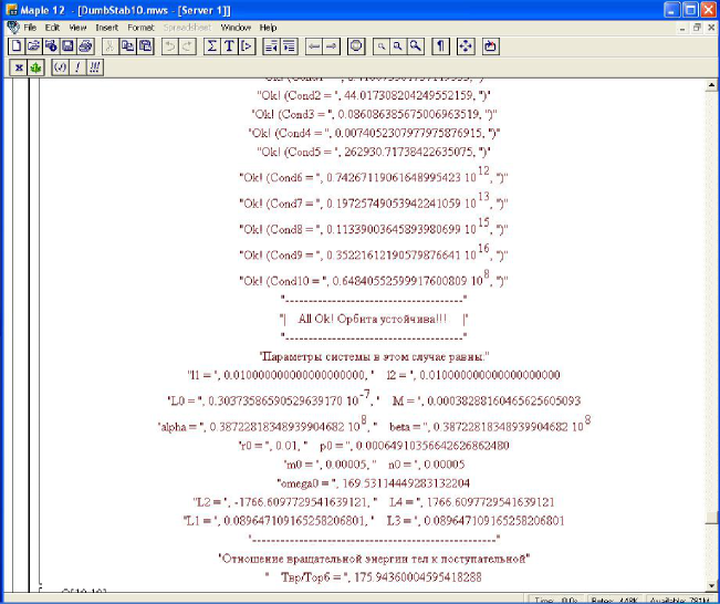
Рис. 1: *

Fig. Test the fulfilment of the theorem conditions for specify orbit

Summary

The paper is devoted to the analytical investigation of the possible existence of orbital motions in the mathematical model [1] which we proposed earlier and which describes the magnetic interaction of rigid bodies.

It has been shown that thanks to the application of group-theoretical methods the Hamiltonian formalism developed in [1] on the basis of Poisson structures is a suitable mathematical instrument for the analytical investigation of the orbital motion stability.

The possibility of stable orbital motion has been proved for a specific system.

Ten conditions for the system parameters have been analytically obtained; they make it possible to define the areas of the orbital stability in the parameter space of the system.

Following the logic of the constructive proof it is possible to assert that magnetic systems can form stable orbits. This destroys the widespread opinion [5] about the global instability of magnetic systems.

E-mail address: stah@kipt.kharkov.ua, stah_z@yahoo.com

Received 17.01.2011