Wronskian method for bound states

Abstract

We propose a simple and straightforward method based on Wronskians for the calculation of bound–state energies and wavefunctions of one–dimensional quantum–mechanical problems. We explicitly discuss the asymptotic behavior of the wavefunction and show that the allowed energies make the divergent part vanish. As illustrative examples we consider an exactly solvable model and the Gaussian potential well.

1 Introduction

Wronskians (or Wronskian determinants) are most useful for the analysis of ordinary differential equations in general[1] and the Schrödinger equation in particular[2]. Whitton and Connor[3] applied a remarkable Wronskian formalism to resonance tunnelling reactions and we have recently proposed that a closely related method may be suitable for teaching quantum scattering in advanced undergraduate and graduate courses in quantum mechanics[4].

The purpose of this paper is to show that the Wronskian method is also useful for the study of bound states of one–dimensional quantum–mechanical models. We believe that this variant of the approach is also suitable for pedagogical purposes and enables a unified treatment of the discrete and continuous spectra of simple quantum–mechanical models.

In section 2 we convert the Schrödinger equation into a dimensionless eigenvalue equation and show how to apply the Wronskian method to bound states. In section 3 we illustrate the application of the approach by means of two suitable examples. In section 4 we outline the main results of the paper and draw conclusions. Finally, in an Appendix we outline the main properties of Wronskians that are relevant to present discussion.

2 The Schrödinger equation

Before solving the Schrödinger equation it is a good practice to convert it into a dimensionless eigenvalue equation. In this way one removes all the physical constants and reduces the number of model parameters to a minimum. The time–independent Schrödinger equation for a particle of mass $m$ that moves in one dimension ($-\infty<X<\infty$) under the effect of a potential $V(X)$ is

$$-\frac{\hbar^{2}}{2m}\psi^{\prime\prime}(X)+V(X)\psi(X)=E\psi(X)$$ (1)

where a prime indicates derivative with respect to the coordinate. If we define the dimensionless coordinate $x=X/L$, where $L$ is an appropriate length scale, then we obtain the dimensionless eigenvalue equation

$$-\frac{1}{2}\varphi^{\prime\prime}(x)+v(x)\varphi(x)=\epsilon\varphi(x)$$

$$\varphi(x)=\sqrt{L}\psi(Lx),\;v(x)=\frac{mL^{2}}{\hbar^{2}}V(Lx),\;\epsilon=\frac{mL^{2}E}{\hbar^{2}}$$ (2)

The length unit $L$ that renders both $\epsilon$ and $v(x)$ dimensionless is arbitrary and we can choose it in such a way that makes the Schrödinger equation simpler. We will see some examples in section 3.

It is well known that a general solution to the second–order differential equation (2) can be written as a linear combination of two linearly independent solutions. Here we write

$$\varphi(x)=A_{2}C(x)+B_{2}S(x)$$ (3)

where the solutions $C(x)$ and $S(x)$ satisfy

$$C(x_{0})=S^{\prime}(x_{0})=1,\;C^{\prime}(x_{0})=S(x_{0})=0$$ (4)

at a given point $x_{0}$ in $(-\infty,\infty)$. These conditions are sufficient to ensure that $C(x)$ and $S(x)$ are linearly independent[2].

For every value of the dimensionless energy $\epsilon$ we know that

$$\varphi(x)\rightarrow\left\{\begin{array}[]{c}A_{1}L_{c}(x)+B_{1}L_{d}(x),\,x\rightarrow-\infty\\ A_{3}R_{c}(x)+B_{3}R_{d}(x),\,x\rightarrow\infty\end{array}\right.$$ (5)

where $L$ and $R$ stand for left and right and $c$ and $d$ for convergent and divergent, respectively. It means that, for arbitrary $\epsilon$, the wavefunction is a linear combination of a convergent and a divergent function when $|x|\rightarrow\infty$. If, for a particular value of $\epsilon$, $B_{1}=B_{3}=0$ then the resulting wavefunction is square integrable. In other words, this condition determines the energies of the discrete spectrum.

It follows from the Wronskian properties outlined in the Appendix that

$$B_{1}W(L_{c},L_{d}) = A_{2}W(L_{c},C)+B_{2}W(L_{c},S),\;x\rightarrow-\infty$$

$$B_{3}W(R_{c},R_{d}) = A_{3}W(R_{c},C)+B_{2}W(R_{c},S),\;x\rightarrow\infty$$ (6)

Therefore, when $B_{1}=B_{3}=0$ we have a linear homogeneous system of two equations with two unknowns: $A_{2}$ and $B_{2}$. There will be nontrivial solutions provided that its determinant vanishes

$$W(L_{c},C)W(R_{c},S)-W(R_{c},C)W(L_{c},S)=0$$ (7)

The roots of this equation $\epsilon_{n}$, $n=0,1,\ldots$ are the energies of the bound states (discrete spectrum).

When the potential is parity invariant

$$v(-x)=v(x)$$ (8)

and $x_{0}=0$ then $C(x)$ and $S(x)$ are even and odd functions, respectively. In this case we have

$$W(L_{c},S) = W(R_{c},S)$$

$$W(L_{c},C) = -W(R_{c},C)$$ (9)

and the determinant (7) takes a simpler form: $W(R_{c},C)W(R_{c},S)=0$. We appreciate that the even and odd solutions are clearly separate and their eigenvalues are given by

$$W(R_{c},C) = 0$$

$$W(R_{c},S) = 0$$ (10)

respectively. Besides, we need to consider only the interval $0\leq x<\infty$.

Commonly, it is not difficult to derive approximate expressions for the convergent and divergent asymptotic forms of the wavefunction because they are straightforwardly determined by the asymptotic behavior of the potential $v(x)$. Therefore, it only remains to have sufficiently accurate expressions for $C(x)$ and $S(x)$ and their derivatives in order to obtain the eigenvalues by means of equation (7). This problem is easily solved by means of, for example, a suitable numerical integration method[5]. If $y(x)$ stands for either $C(x)$ or $S(x)$ then such an approach gives us its values at a set of points $x_{0}-N_{L}h,\,x_{0}-N_{L}h+h,\ldots,\,x_{0},\,x_{0}+h,\ldots,\,x_{0}+N_{R}h$ where $N_{L}$ and $N_{R}$ are the number of steps of size $h$ to the left and right of $x_{0}$, respectively. The number of steps should be sufficiently large so that $y(x)$ reaches its asymptotic value at both $x_{L}=x_{0}-N_{L}h$ and $x_{R}=x_{0}+N_{R}h$ and $h$ should be sufficiently small to provide a good representation of $y(x)$. The numerical integration methods also yield the derivative of the function $y^{\prime}(x)$ at the same set of points which facilitates the calculation of the Wronskians.

3 Examples

In order to test the accuracy of the Wronskian method we first choose the exactly solvable problem given by the potential $V(X)=-V_{0}/\cosh^{2}(\alpha X)$, where $V_{0}>0$ and $\alpha>0$. If we set $L=1/\alpha$ we are led to the dimensionless Schrödinger equation (2) where

$$v(x) = -\frac{v_{0}}{\cosh^{2}(x)},\;$$

$$v_{0} = \frac{mV_{0}}{\hbar^{2}\alpha^{2}},\;\epsilon=\frac{mE}{\hbar^{2}\alpha^{2}}$$ (11)

Note that the dimensionless energy $\epsilon$ depends on only one independent potential parameter $v_{0}$. The units of length and energy are $1/\alpha$ and $\hbar^{2}\alpha^{2}/m$, respectively, and we do not have to bother about the mass of the particle and the Planck constant when solving the differential equation. The allowed dimensionless energies are given by[6]

$$\epsilon_{n} = -\frac{1}{2}(\lambda-1-n)^{2},\;n=0,1,\ldots\leq\lambda-1$$

$$\lambda = \frac{1}{2}\left(1+\sqrt{1+8v_{0}}\right)$$ (12)

and the spectrum is continuous for all $\epsilon>0$. It is clear that $\lambda\rightarrow 1$ as $v_{0}\rightarrow 0$ and there is only one bound state when $1<\lambda<2$ ($0<v_{0}<1$). As $v_{0}$ increases more bound states appear. As a result there are critical values of the potential parameter for which $\epsilon_{n}=0$ that are given by the condition $\lambda_{n}=n+1$ or $v_{0,n}=\lambda_{n}(\lambda_{n}-1)/2=n(n+1)/2$.

Since $\lim_{|x|\rightarrow\infty}v(x)=0$ then in this case $R_{c}(x)=e^{-kx}$ and $R_{d}(x)=e^{kx}$, where $k^{2}=-2\epsilon$ (we only consider the interval $0\leq x<\infty$ because the potential is parity invariant). Consequently, the allowed energies are determined by the conditions

$$W(R_{c},C) = \left[C^{\prime}(x)+kC(x)\right]e^{-kx}=0,\;x\rightarrow\infty$$

$$W(R_{c},S) = \left[S^{\prime}(x)+kS(x)\right]e^{-kx}=0,\;x\rightarrow\infty$$ (13)

for even and odd states, respectively.

Since the potential (11) is parity invariant we integrate the Schrödinger equation from $x_{0}=0$ to $x_{R}=N_{R}h$. Fig. 1 shows the Wronskians $W(R_{c},C)$ and $W(R_{c},S)$ for $\epsilon=-1$ and $v_{0}=2.5$.

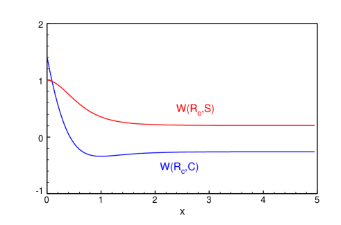
Figure 1: Wronskians for the exactly solvable problem with $\epsilon=-1$ and $v_{0}=2.5$

We appreciate that $x=x_{R}=5$ is large enough to have constant asymptotic Wronskians and we choose this coordinate value from now on. This numerical test also shows that it is sufficient for present purposes to set $h=0.01$ and $N_{R}=500$ in the fourth–order Runge–Kutta method[5] built in the computer algebra system Derive (http://www.chartwellyorke. com/derive.html).

Fig. 2 shows both $W(R_{c},C)$ and $W(R_{c},S)$ for $x=5$ and $v_{0}=6$ as functions of $\epsilon$. We see that the Wronskians vanish at the exact eigenvalues given by equation (12). This is a confirmation of our earlier assumption that the number of steps and their size are suitable for obtaining reasonable results.

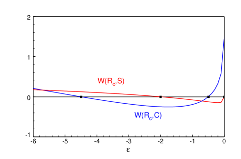
Figure 2: Wronskians for the exactly solvable problem with $v_{0}=6$ as functions of $\epsilon$. Squares mark the exact eigenvalues

Fig. 3 shows $W(R_{c},C)$ and $W(R_{c},S)$ for $x=5$ and $\epsilon=0$ as functions of $v_{0}$. In this case the Wronskians vanish at the exact critical values $v_{0,n}=n(n+1)/2$.

Figure 3: Wronskians for the exactly solvable problem with $\epsilon=0$ as functions of $v_{0}$. Squares mark the exact critical parameters

Those results for the exactly solvable problem suggest that the Wronskian method is successful for all bound–state energies and all well depths. As a second example, in what follows we try the nontrivial problem provided by the Gaussian well $V(x)=-V_{0}e^{-\alpha X^{2}}$, where $V_{0}>0$, and $\alpha>0$, that we easily convert into the dimensionless potential

$$v(x) = -v_{0}e^{-x^{2}},$$

$$v_{0} = \frac{mV_{0}}{\hbar^{2}\alpha},\;\epsilon=\frac{mE}{\hbar^{2}\alpha}$$ (14)

by means of the length unit $L=1/\sqrt{\alpha}$. This potential is also parity invariant and vanishes asymptotically as $|x|\rightarrow\infty$ so that the calculation is similar to the preceding example. In order to show that the Wronskian method also applies successfully to this model we first obtain some critical values of the potential parameter $v_{0}$. Fig. 4 shows $W(R_{c},C)$ and $W(R_{c},S)$ for $x=5$ and $\epsilon=0$ as functions of $v_{0}$. The three zeros of the Wronskians shown in the figure appear at $v_{0,1}=1.342$, $v_{0,2}=4.325$ and $v_{0,3}=8.898$.

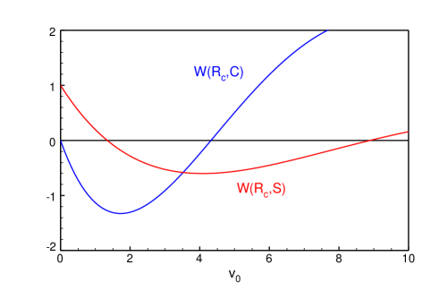
Figure 4: Wronskians for the Gaussian well with $\epsilon=0$ as functions of $v_{0}$

The numerical methods, although as accurate as one may desire (or the computer allows) , are not exact; therefore we can make the coefficient of the divergent part of the wavefunction very small but never exactly equal to zero. To illustrate this point we consider the ground state of the Gaussian well with $v_{0}=5$ and obtain the approximate energy $\epsilon_{0}=-3.6077$ by means of a naive bracketing algorithm. The Wronskian method gives us the coefficient of the divergent part of the wavefunction $B_{3}=W(R_{c},C)/W(R_{c},R_{d})=W(R_{c},C)/(2k)=1.886\times 10^{-6}$ as a by–product of the calculation at $x=5$. Note that in this case $A_{2}=1$ and $B_{2}=0$ so that $C(x)$ is the unnormalized approximation to $\varphi_{0}$. Fig. 5 shows that the wavefunction decreases as $A_{3}e^{-kx}$ to almost zero and then increases as $B_{3}e^{kx}$. For intermediate values of the coordinate the convergent part dominates because $A_{3}$ is much larger that $B_{3}$ but for larger values of $x$ $R_{d}$ dominates as shown in Fig. 5. The points in this figure are the values of $B_{3}R_{d}=1.886\times 10^{-6}e^{2.686x}$.

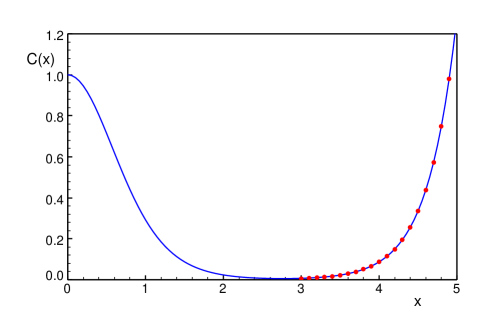
Figure 5: Unnormalized ground–state wavefunction for the Gaussian well with $v_{0}=5$

We can improve the calculation and make $B_{3}$ as small as desired, but it will never be exactly zero because the numerical calculation is approximate and the spurious divergent part will always be present. However, in order to normalize the wavefunction and calculate expectation values we judiciously truncate the coordinate interval at a convenient point and obtain finite accurate values for those quantities. The Wronskian method is clearly suitable for deciding on the truncation point and estimating the error.

4 Conclusions

In our opinion the Wronskian method is sufficiently clear and straightforward for teaching an advanced undergraduate or graduate course in quantum mechanics. The mathematics requires no special background beyond an introductory calculus course. Since many available computer softwares offer numerical integration methods the programming effort is relatively light.

From a purely theoretical point of view the method is suitable for the discussion of the convergent and divergent asymptotic behaviors of the wavefunction and for illustrating how the allowed bound–state energies make the divergent part vanish leading to square–integrable wavefunctions. The students may try other quantum–mechanical models, derive the appropriate asymptotic behaviors analytically and then test their results by means of a suitable computer program. They can verify that the Wronskians already approach constants as the absolute value of the coordinate increases and that the wavefunction already looks like a square integrable function when the coefficient of the divergent contribution is almost zero. They can even estimate the remnants of the asymptotic divergent part because the Wronskian method provides the necessary coefficients.

In addition to it, the Wronskian method is also suitable for quantum scattering[4] allowing a unified treatment of both the discrete and continuous spectra of the model.

Finally, we point out that computer algebra systems are remarkable aids for the teaching and learning process because they facilitate the algebraic treatment of the problem and even offer the possibility of straightforward numerical calculations (although they are considerably slower than specialized numerical programs).

Appendix A Wronskians

In order to make this paper sufficiently self–contained in this appendix we outline some well known results about the Wronskians that are useful for the study of ordinary differential equations in general[1] and also for the treatment of the Schrödinger equation in particular[2, 3]. To this end, we consider the ordinary second–order differential equation

$$L(y)=y^{\prime\prime}(x)+Q(x)y(x)=0$$ (15)

If $y_{1}$ and $y_{2}$ are two linearly independent solutions to this equation then we have

$$y_{1}L(y_{2})-y_{2}L(y_{1})=\frac{d}{dx}W(y_{1},y_{2})=0$$ (16)

where

$$W(y_{1},y_{2})=y_{1}y_{2}^{\prime}-y_{2}y_{1}^{\prime}$$ (17)

is the Wronskian (or Wronskian determinant[1]). The Wronskian is a skew–symmetric

$$W(f,g)=-W(g,f)\Rightarrow W(f,f)=0$$ (18)

and linear function of its arguments

$$W(f_{1}+f_{2},g) = W(f_{1},g)+W(f_{2},g)$$

$$W(cf,g) = cW(f,g)$$ (19)

where $c$ is a constant.

By linear combination of $y_{1}(x)$ and $y_{2}(x)$ we easily obtain two new solutions $C(x)$ and $S(x)$ satisfying

$$C(x_{0})=S^{\prime}(x_{0})=1,\;C^{\prime}(x_{0})=S(x_{0})=0\;$$ (20)

at a given point $x_{0}$ so that $W(C,S)=1$ for all $x$. If we write the general solution to equation (15) as

$$y(x)=AC(x)+BS(x)$$ (21)

then

$$A=W(y,S),\;B=W(C,y)$$ (22)

This equation is quite useful for deriving relationships between the coefficients of the asymptotic expansions of the wavefunction in different regions of space as shown in sections 2 and 3. Additional mathematical properties of the Wronskians are available in Powell and Crasemann’s book on quantum mechanics[2].

References

- [1] T. M. Apostol, Calculus, Second ed. (Blaisdell, Waltham, Massachusetts, 1969).
- [2] J. L. Powell and B. Crasemann, Quantum Mechanics, (Addison-Wesley, Reading, Massachussetts, 1961).
- [3] W. N. Whitton and J. N Connor, L., ”Wronskian analysis of resonance tunneling reactions”, Mol. Phys. 26, 1511-1520 (1973).
- [4] F. M. Fernández, ”Quantum scattering by Wronskians”, arXiv:1101.0957v1 [quant-ph].
- [5] W.H. Press, B. P. Flannery, S. A. Teulosky et al., Numerical recipes. The art of scientific computing, (Cambridge University Press, Cambridge, 1986).
- [6] S. Flügge, Practical Quantum Mechanics, (Springer-Verlag, Berlin, 1999).