Properties of nano-pattern formation in reaction-diffusion systems with hyperbolic transport and multiplicative noise

Abstract

We study nano-pattern formation in a stochastic model for adsorption-desorption processes with interacting adsorbate and hyperbolic transport caused by memory effects. It is shown that at early stages the system manifests pattern selection processes. Stationary stable patterns of nano-size are analyzed. It was found that multiplicative noise satisfying fluctuation-dissipation relation can induce re-entrant pattern formation related to non-equilibrium transitions. According to obtained Fokker-Planck equation kinetics of island sizes in a quasi-stationary limit is discussed. Analytical results are compared with computer simulations.

1 Introduction

From theoretical and experimental observations it is known that reaction-diffusion systems play an important role in the study of generic spatiotemporal behavior of non-equilibrium systems. Usually such models admit main contributions related to both local dynamics (chemical reactions type of birth-and-death processes) and mass transport. Novel experimental methods, such as field ion microscopy, scanning tunneling microscopy can be used to monitor chemical reactions on the metal surfaces with atomic resolution.

In adsorption-desorption processes when material can be deposited from the gaseous phase such experimental methods allow one to investigate formation of clusters or islands of adsorbed molecules/atoms [1]. Such islands can have linear size of nanometer range [2]. In Refs.[3, 4, 5, 6, 7] it was experimentally shown that nano-patterns on solid surface and nano-islands in adsorbed mono-atomic layers can be organized. It was found that lateral interactions between adsorbate play an important role in processes of pattern formation on metal surfaces. The adsorbate presence can modify the local crystallographic structures of the substrate’s surface layer producing long range interactions between adsorbed atoms and their clusters (see for example, Refs.[8, 9, 10]). It was observed experimentally that nanometer-sized vacancy islands can be organized in a perfect triangular lattice when a single monolayer of Ag was exposed on Ru(0001) surface at room temperature [7]. The origin of such self-organization of vacancy islands is an elastic interaction between edges of neighboring islands [7]. Such systems can be widely used in electronic devices in industrial applications. Despite theoretical studies of nano-patterns were widely reported (see Refs.[11, 12, 13, 14, 15, 16] and citations therein) no detailed descriptions of elastic effects leading to formation vacancy/adsorbate islands lattice were presented.

It is known that such kind of processes can be studied by multiscale modeling including: ab-initio calculations allowing one to set parameters of primitive cell at zero temperature and some energetic parameters; molecular dynamics simulations monitoring microscopic processes of interactions of atoms; Monte-Carlo approach studying physics on bigger time scales. Unfortunately the corresponding computational time remains excessive and presented methods can be used to describe the system only on micron scales. To study pattern-forming transitions one can use mesoscopic approach to modelize self-organization processes on large sizes. It can be generalized by taking into account corresponding fluctuating sources representing an influence of a microscopic level or fluctuations of environment [11, 12].

Properties of pattern formation in systems of adsorption-desorption type with dissipative dynamics were studied previously [11, 12]. Pattern formation in stochastic systems with internal multiplicative noise obeying fluctuation-dissipation relation was discussed in Refs.[13, 16, 17]. It was shown that internal multiplicative noise can sustain stationary patterns of nano-size range; the corresponding patterning processes are well related to non-equilibrium transitions induced by internal multiplicative noise (entropy driven phase transitions [18, 19, 20, 21, 22]).

Recently modifications of this mesoscopic approach were proposed, where in the framework of continuous model one can describe processes at microscopic and diffusion scales. This approach is known in literature as modified phase field crystals method [23, 24, 25, 26]. It can be used to study crystal growth, solidification processes, motion of defects, phase transitions in crystalline systems (having special kind of order). Its main advantage is in introduction of a crystalline order with elastic interactions leading to formation of crystal lattice and of inertia effects related to a finite propagation speed [27, 28, 29]. Inertial contribution is essential at early stages in the system dynamics. On the diffusion time scale one can observe patterning with a formation of crystalline lattice regarding to the Hook’s law. Formally, the elastic effects are modelized by expansion of a pair interatomic potential in the Fourier space up to the fourth order in wave-numbers [23, 24, 30]. As a result the spatial interactions are described by the Swift-Hohenberg operator $(q_{0}^{2}+\nabla^{2})^{2}$, $\nabla\equiv\partial/\partial\mathbf{r}$, $q_{0}$ is a constant related to period of spatial patterns. Influence of both internal and external stochastic sources onto pattern-forming transitions in crystalline systems were discussed in Refs.[31, 32]. It was shown that in such kind of systems due to finite propagation speed pattern selection processes are possible; the external noise can principally change topology of patterns realized in a pure deterministic case.

For class of systems with adsorption-desorption and diffusion processes the typical deterministic equation, which will interest us is of the form

$$\partial_{t}x=f(x)-\nabla\cdot\mathbf{J},$$ (1)

where $x=x(\mathbf{r},t)$ is the local coverage at surface defined as the quotient between the number of adsorbed molecules/atoms in a cell of the surface and the fixed number of available sites in each cell, $x\leq 1$. The term $f(x)$ stands for local dynamics and describes birth-and-death or adsorption-desorption processes; the flux $\mathbf{J}$ represents the mass transport.

Most of the theoretical studies deal with the standard Fick law $\mathbf{J}=-D\nabla x$, $D$ is the diffusion constant. It is known that at $f=0$ the ordinary diffusion equation $\partial_{t}x=\nabla\cdot D\nabla x$ has the unrealistic feature of infinitely fast (infinite) propagation. To avoid such unphysical situation the diffusion flux can be generalized by taking into account memory (non-equilibrium) effects

$$\mathbf{J}=-\int\limits_{0}^{t}M(t,t^{\prime})D\nabla x(\mathbf{r},t^{\prime}){\rm d}t^{\prime}$$ (2)

described by the memory kernel $M(t,t^{\prime})=\tau_{J}^{-1}\exp(-|t-t^{\prime}|/\tau_{J})$. In such a case in the limit $f(x)=0$ one gets the finite propagation speed $\sqrt{D/\tau_{J}}$. At $\tau_{J}\to 0$ the assymptotic $M(t,t^{\prime})=\delta(t-t^{\prime})$ leads to the Fick law $\mathbf{J}=-D\nabla x$ with infinite propagation. As far as real systems (molecules, atoms) have finite propagation speed one should use Eq.(2) or the equivalent Maxwell-Cattaneo equation: $\tau_{J}\partial_{t}\mathbf{J}=-\mathbf{J}-D\nabla x$ [28]. Equations (1,2) can be combined into one equation of the form

$$\tau_{J}\partial^{2}_{tt}x+(1-\tau_{J}f^{\prime}(x))\partial_{t}x=f(x)+\nabla\cdot D(x)\nabla x,$$ (3)

where prime denotes derivative with respect to the argument. As was pointed out in Ref.[28] this equation has some restrictions: (i) it typically does not preserve positivity of the solution $x(\mathbf{r},t)$; (ii) the damping coefficient must be positive, i.e., $f^{\prime}(x)<\tau_{J}^{-1}$.

In this study we are aimed to describe pattern formation processes in system given by Eq.(3) generalized by introducing multiplicative noise satisfying fluctuation-dissipation relation. We use suppositions of the phase field theory to construct effective model describing formation of nano-patterns with crystalline order and pattern selection processes. It will be shown that formation of stationary patterns in stochastic systems is well related to noise-induced effects, namely, non-equilibrium transitions. We shall argue that noise correlated in time can induce re-entrant ordering processes, where the stable or unstable patterns are realized in a window of control parameter values. Studying behavior of islands size as clusters of dense phase and vacancy islands of diluted phase we obtain its time asymptotics. Analytical results are verified by computer simulations.

The paper is organized as follows. In Section 2 we describe the model of our system. Section 3 is devoted to study stability of patterns at early stages. In section 4 we derive the effective Fokker-Planck equation to study noise induced effects in Section 5 and formation of stationary patterns in Section 6. In Section 7 we discuss evolution of islands size. We prove our analytical results by computer simulation in Section 8. Finally, conclusions are presented in last section.

2 The model

We consider a model where only one class of particles is possible. Following Refs.[13, 16, 11, 12, 35, 33, 34] one assumes that the particles can be adsrobed, desorbed, can diffuse and interact among themselves. Therefore, we introduce the scalar field describing dynamics of the local coverage at surface $x(\mathbf{r},t)\in[0,1]$. The reaction term incorporates adsorption and desorption terms as follows $f(x)=k_{a}p(1-x)-k_{d}x\exp(U(\mathbf{r})/T)$. Here $k_{a}$ and $k_{d}$ are adsorption and desorption rates, respectively; $p$ is the partial pressure of the gaseous phase; $U(\mathbf{r})$ is the interaction potential.

The total flux $\mathbf{J}$ is a sum of both ordinary diffusion flux $(-D_{0}\nabla x)$ and flow of adsorbate $(-(D_{0}/T)x(1-x)\nabla U)$. Here the multiplier $x(1-x)$ denotes that the flux is only possible to the $(1-x)$ free sites. Using the phase field crystals methodology [23, 24, 30] for the potential $U$ one assumes

$$U(\mathbf{r})/T=-\int{\rm d}\mathbf{r}^{\prime}u(\mathbf{r}-\mathbf{r}^{\prime})x(\mathbf{r}^{\prime})\simeq-\varepsilon x-\mu\nabla^{2}x-\varkappa\nabla^{4}x,$$ (4)

where $\varepsilon\equiv T^{-1}\int{\rm d}ru(r)$, $\mu\equiv(1/2T)\int{\rm d}rr^{2}u(r)$ and $\varkappa\equiv(1/4T)\int{\rm d}rr^{4}u(r)$. To estimate $\varepsilon$, $\mu$ and $\varkappa$ one can suppose that there is maximal intensity $u(0)=u_{max}$ and characteristic radius $r_{0}$ [12], therefore, one has $\varepsilon\simeq u_{max}r_{0}^{2}$, $\mu\simeq\varepsilon r_{0}^{2}$, $\varkappa\simeq\mu r_{0}^{2}$. The obtained expression can be rewritten in a more simplest form $U(\mathbf{r})/T\simeq-(1/4\varepsilon)\mathcal{L}_{SH}x$, where $\mathcal{L}_{SH}\equiv(q_{0}^{2}+\nabla^{2})^{2}$ is the Swift-Hohenberg spatial coupling operator where $q_{0}^{2}=\varepsilon/\varkappa$; here we take $\mu=1$ that results to relations: $\varkappa=1/4\varepsilon$, $q_{0}^{2}=4\varepsilon^{2}$.

Next, after substitution of all above terms we get a system of two equations kind of (1, 2) with

$$f(x)=\alpha(1-x)-x\exp(-\varepsilon x),\quad\alpha\equiv k_{a}p/k_{d},$$ (5)

where the total diffusion flux $\mathbf{J}$ satisfies the following relaxation equation

$$\tau_{J}\partial_{t}\mathbf{J}=-\mathbf{J}-D_{0}[\nabla x-G(x)\nabla\mathcal{L}_{SH}x];\quad G(x)=\frac{1}{4\varepsilon}x(1-x).$$ (6)

The equivalent equation for the coverage takes the form

$$\tau_{J}\partial^{2}_{tt}x+\gamma(x)\partial_{t}x=f(x)+D_{0}\nabla\cdot[\nabla x-G(x)\nabla\mathcal{L}_{SH}x],$$ (7)

where $\gamma(x)\equiv 1-\tau_{J}f^{\prime}(x)$. In our stochastic analysis we are based on this equation generalized by introduction of a multiplicative noise in ad hoc form using the fluctuation dissipation relation. Therefore, the corresponding Langevin dynamics is described by the equation

$$\tau_{J}\partial^{2}_{tt}x+\gamma(x)\partial_{t}x=\varphi(x;\nabla)+g(x)\zeta(\mathbf{r},t).$$ (8)

Here $\varphi(x;\nabla)\equiv f(x)+D_{0}\nabla\cdot[\nabla x-G(x)\nabla\mathcal{L}_{SH}x]$; $\gamma(x)\equiv g^{2}(x)$ in order to guarantee that the fluctuation-dissipation relation is satisfied [36]; $\zeta$ represents Langevin force. From the mathematical viewpoint a generalized Langevin equation defined with a memory kernel has a noise fulfilling the fluctuation-dissipation relation with the noise time-correlator as the memory kernel has. Therefore, in our case the memory kernel is reduced to the delta-function and hence, the process $\zeta$ is a white noise in time (with a zero correlation time, $\tau_{c}=0$). It is known that mathematically defined white noise (with delta-correlation function) has no physical meaning [37], for example: every next value for $\zeta$ does not depend on it previous value; a spread in values of the noise $\zeta$ and a total power of the noise are infinite. Therefore, one needs to consider physical fluctuation source having small but finite correlation time $\tau_{c}\ll 1$ (see, for example [38]). Hence, in our study we consider a generalized model of the Gaussian noise with zero mean and a correlator

$$\langle\zeta(\mathbf{r},t)\zeta(\mathbf{r}^{\prime},t^{\prime})\rangle=\frac{2\sigma^{2}}{\tau_{c}}\exp\left(-\frac{|t-t^{\prime}|}{\tau_{c}}\right)\delta(\mathbf{r}-\mathbf{r^{\prime}}),$$ (9)

where $\sigma^{2}$ is the noise intensity. Hence, a set of main functions defining the system behavior is reduced to the reaction term $f(x)$ and the field-dependent diffusion coefficient $G(x)$.

3 Linear stability analysis

Let us study fluctuation effects at early stages. The stability analysis for the system can be done considering a behavior of the averaged quantity $\langle x\rangle$ in the vicinity of the state $x_{0}$ related to unique minimum position of a bare potential $V(x)=-\int_{0}^{x}{\rm d}x^{\prime}f(x^{\prime})$. Averaging Eq.(8) one gets

$$\tau_{J}\partial^{2}_{tt}\langle x\rangle+\left<\gamma(x)\partial_{t}x\right>=\left<f(x)+D_{0}\nabla\cdot[\nabla x-G(x)\nabla\mathcal{L}_{SH}x]\right>+\left<g(x)\zeta(\mathbf{r},t)\right>.$$ (10)

Making use of the Novikov theorem [39], for the noise correlator we have $\left<g(x)\zeta(\mathbf{r},t)\right>=(\sigma^{2}/2)\left<\gamma^{\prime}(x)\right>$. Therefore, in the vicinity of the state $x_{0}$ for the Fourier component $\langle\delta x_{\mathbf{k}}(\omega)\rangle$ of the quantity $\langle\delta x\rangle=\langle x(\mathbf{r},t)\rangle-x_{0}$ the dispersion relation takes the form

$$-\tau_{J}\omega^{2}-{\rm i}\gamma(x_{0})\omega=f^{\prime}(x_{0})-D_{0}k^{2}(1-G(x_{0})[q_{0}^{2}-k^{2}]^{2})-\frac{\tau_{J}\sigma^{2}}{2}f^{\prime\prime\prime}(x_{0}).$$ (11)

It leads to the following dependencies for dispersion curves:

$$\omega(k)_{\mp}=-\frac{{\rm i}\gamma(x_{0})}{2\tau_{J}}\mp\left[\frac{D_{0}k^{2}(1-G(x_{0})[q_{0}^{2}-k^{2}]^{2})-f^{\prime}(x_{0})}{\tau_{J}}+\frac{\sigma^{2}}{2}f^{\prime\prime\prime}(x_{0})-\frac{\gamma^{2}(x_{0})}{4\tau^{2}_{J}}\right]^{1/2}.$$ (12)

One can see that $\omega(k)$ can have real and imaginary parts, i.e. $\omega(k)=\Re\omega(k)\pm{\rm i}\Im\omega(k)$. The component $\Re\omega(k)$ is responsible for oscillatory solutions, whereas $\Im\omega(k)$ describes a stability of the solution $\langle\delta x_{\mathbf{k}}(\omega)\rangle$. Analysis of both $\Re\omega(k)$ and $\Im\omega(k)$ allows us to set a threshold for a wave-number where oscillatory solutions are possible, from one hand, and, from another one, to define a wave-number for the first unstable solution. From the obtained dispersion relations it follows that at $k=k_{0}$ satisfying equation

$$k_{0}^{2}(1-G(x_{0})[q_{0}^{2}-k_{0}^{2}]^{2})=\frac{1}{D_{0}}\left[f^{\prime}(x_{0})-\frac{\sigma^{2}\tau_{J}}{2}f^{\prime\prime\prime}(x_{0})+\frac{\gamma^{2}(x_{0})}{4\tau_{J}}\right]$$ (13)

two branches of the dispersion relation degenerate. The unstable mode appears at $k=k_{c}$ obtained from the equation

$$k_{c}^{2}(1-G(x_{0})[q_{0}^{2}-k_{c}^{2}]^{2})=\frac{1}{D_{0}}\left[f^{\prime}(x_{0})-\frac{\sigma^{2}\tau_{J}}{2}f^{\prime\prime\prime}(x_{0})\right].$$ (14)

From Eq.(11) it follows that a sign of the effective control parameter $\varepsilon_{ef}\equiv f^{\prime}(x_{0})-(\tau_{J}\sigma^{2}/2)f^{\prime\prime\prime}(x_{0})$ defines stability of the system. Moreover, as far as the sign of $\varepsilon_{ef}$ depends on the reaction term derivatives in the vicinity of the state $x_{0}$, one can conclude that noise-induced effects in the linear regime are possible at $\tau_{J}\neq 0$ and $f^{\prime\prime\prime}(x_{0})\neq 0$.

To make a quantitative analysis we consider firstly stability of the deterministic system setting $\sigma^{2}=0$ in the vicinity of the unique minimum position $x_{0}$ of $V(x)$. As far as $q_{0}$ increases with the lateral interaction energy, next, we take small values for $\varepsilon$ and study two cases related to small and large values for the adsorption rate. The corresponding dependencies of $\Re\omega(k)$ and $\Im\omega(k)$ are shown in Fig.1.

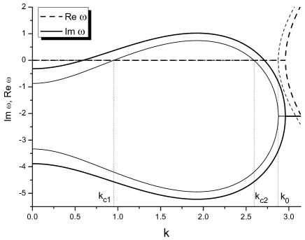
a) b)

Figure 1: Real and imaginary parts of the dispersion relation $\omega(k)$ for deterministic and stochastic systems (thin and thick lines, respectively) at $\varepsilon=2.5$, $D_{0}=1$, $\tau_{J}=0.3$: a) $\alpha=0.03323$, $x_{0}=0.035$ (thin and thick lines relate to $\sigma^{2}=0$ and $\sigma^{2}=0.2$, respectively); b) $\alpha=0.4055$, $x_{0}=0.75$ (thin and thick lines relate to $\sigma^{2}=0$ and $\sigma^{2}=0.1$, respectively)

From Fig.1a obtained in the vicinity of diluted phase characterized by $x_{0}\to 0$ modes with wave-numbers $k>k_{0}$ manifest decaying oscillations (here $\Re\omega_{+}(k)=-\Re\omega_{-}(k)\neq 0$, $\Im\omega_{+}(k)<0$). Inside both intervals $k\in[0,k_{c1}]$ and $k\in[k_{c2},k_{0}]$ the corresponding modes are stable without oscillations (here $\Re\omega_{\pm}(k)=0$, $\Im\omega_{\pm}(k)<0$). In the domain $k\in(k_{c1},k_{c2})$ unstable modes characterized by $\Im\omega_{+}(k)>0$ and $\Re\omega_{\pm}(k)=0$ appear. In the vicinity of the dense phase with $x_{0}\to 1$ (see Fig.1b) there are no oscillatory solutions due to $\Re\omega_{\pm}(k)=0$, but unstable modes can be realized. Here at small wave-numbers one has $\Im\omega_{\pm}(k<k_{c})<0$, whereas at $k>k_{c}$ all modes are unstable in the linear regime with $\Im\omega_{+}(k)>0$. In the stochastic case ($\sigma^{2}\neq 0$) in the vicinity of the diluted phase the noise action results in a decrease of the number of oscillating modes shifting $k_{0}$ toward $\pi$; the interval for unstable modes $[k_{c1},k_{c2}]$ enlarges (see thick lines in Fig.1a). In the vicinity of the dense phase the noise shifts position of the critical wave-number $k_{c}$ toward small $k$ increasing the number of unstable modes (see thick lines in Fig.1b).

In Figure 2 we plot stability diagram $\alpha(k))$ at fixed $\varepsilon$ for both deterministic and stochastic cases.

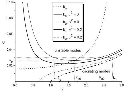
Figure 2: Dependencies $\alpha(k)$ at $\sigma^{2}=0$ (thin lines) and $\sigma^{2}=0.2$ (thick lines). Other parameters are: $\varepsilon=2.5$, $D_{0}=1$, $\tau_{J}=0.3$. Domains of unstable modes and stable oscillating modes are bounded by solid and dashed lines, respectively.

Here above solid lines (thin for the noiseless case and thick for the stochastic one) the corresponding modes with $k\in[k_{c1},k_{c2}]$ are unstable. Below dashed lines the stable modes manifest oscillating behavior. The first unstable mode $k_{c0}$ is realized when equation $\Im\omega(k)_{+}=0$ has unique nonzero solution $k_{c0}$. At small lateral interaction strength of the adsorbate and small adsroption rate only stable modes without oscillations and stable oscillating modes can be formed. Above the threshold $\alpha_{th}=\alpha(k_{c0})$ unstable modes appear leading to spatial self-organization of the adsorbate. When the noise intensity increases above pattern forming processes can be observed at lower value for the adsorption rate; the corresponding patterns are characterized by large wave-lengths then in the noiseless case. The thick dotted line denotes the dependence of the wave-number $k_{m}$ related to a position of the maximum for $\Im\omega(k)_{+}$. At $k>k_{c0}$ the corresponding value $k_{m}$ defines the most unstable mode giving a period of the spatial structure. The most unstable mode at $k>k_{c0}$ is characterized by

$$k_{m}^{2}=\frac{q_{0}^{2}}{3}\left(2-\sqrt{1+\frac{3}{q_{0}^{2}G(x_{0})}}\right).$$ (15)

It follows that $k_{m}$ depends only on the adsorption rate and the lateral interaction energy. The noise action leads to a change in the position of the point $k_{c0}$ lying in the line $\alpha(k_{m})$.

Dependencies of the period of patterns at different values for lateral interaction energy are shown in Fig.3 as dashed lines $k_{m}(\alpha)$ starting at $k=k_{c0}$ for $\sigma^{2}=0.2$. Here choosing a fixed value for $\varepsilon$ from dependencies $\varepsilon(\alpha)$ one can find both the threshold value $\alpha_{th}$ and the corresponding $k_{c0}$. Above the obtained $k_{c0}$ the related period of patterns $\Lambda=2\pi/k_{m}$ can be found at fixed system parameters. It follows that as the noise intensity increases the unstable modes appear at lower values for both $\alpha$ and $\varepsilon$. At elevated $\varepsilon$ the selected patterns are characterized by small period.

Figure 3: Dependencies $k_{m}(\alpha)$ (see left ordinate axis) as dashed lines starting at $k=k_{c0}$ shown for $\sigma^{2}=0.2$ and threshold values as dependencies $\varepsilon(\alpha)$ (see right ordinate axis) at $\sigma^{2}=0$ and $\sigma^{2}=0.2$ (thin and thick solid lines, respectively). Other parameters are: $D_{0}=1$, $\tau_{J}=0.3$.

As far as the first statistical moment illustrates oscillatory behavior one should expect that processes of pattern selection can be observed in such system. Considering properties of pattern selection we need to find dynamical equation for the structure function $S(\mathbf{k},t)$ as a Fourier transform of the two point correlation function $\langle\delta x(\mathbf{r},t)\delta x(\mathbf{r}^{\prime},t)\rangle$ and to study its oscillatory behavior at small times. To that end we obtain the linearized evolution equation for the Fourier components $\delta x_{\mathbf{k}}(t)$ and $\delta x_{-\mathbf{k}}(t)$ and compute $S(\mathbf{k},t)=\langle\delta x_{\mathbf{k}}(t)\delta x_{-\mathbf{k}}(t)\rangle$. Using Novikov’s theorem, and holding only leading terms in it, one gets a dynamical equation

$$\begin{split}\tau_{J}\partial^{2}_{tt}S(\mathbf{k},t)&+\gamma(x_{0})\partial_{t}S(\mathbf{k},t)\\ &=2\left(f^{\prime}(x_{0})-\frac{\sigma^{2}\tau_{J}}{2}f^{\prime\prime\prime}(x_{0})-D_{0}k^{2}(1-G(x_{0})[q_{0}^{2}-k^{2}]^{2})\right)S(\mathbf{k},t)+2\sigma^{2}\gamma(x_{0}).\end{split}$$ (16)

Its analytical solution can be found in the form $S(\mathbf{k},t)-S_{0}\propto\exp(-i\varpi(\mathbf{k})t)$, where

$$\varpi(k)_{\pm}=-\frac{{\rm i}\gamma(x_{0})}{2\tau_{J}}\pm\sqrt{\frac{2\left(D_{0}k^{2}(1-G(x_{0})[q_{0}^{2}-k^{2}]^{2})-f^{\prime}(x_{0})\right)}{\tau_{J}}+\sigma^{2}f^{\prime\prime\prime}(x_{0})-\frac{\gamma^{2}(x_{0})}{4\tau^{2}_{J}}}.$$ (17)

As in the previous case $\Im\varpi$ is responsible for stability of the system, whereas $\Re\varpi$ relates to pattern selection processes. Unstable modes are defined according to Eq.(14). The quantity $k_{0}$ is determined as solution of the equation

$$k_{0}^{2}(1-G(x_{0})[q_{0}^{2}-k_{0}^{2}]^{2})=\frac{1}{D_{0}}\left[f^{\prime}(x_{0})-\frac{\sigma^{2}\tau_{J}}{2}f^{\prime\prime\prime}(x_{0})+\frac{\gamma^{2}(x_{0})}{8\tau_{J}}\right].$$ (18)

An evolution of the structure function at early stages is shown in Fig.4a.

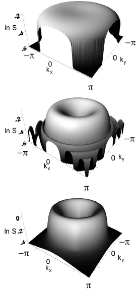
a) b)

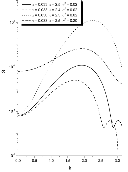
Figure 4: (a) The structure function dynamics at early stages $t=1$, 2.4, 3 (the time is increased from top to bottom) in the vicinity of the state $x_{0}=0.035$ at $\varepsilon=2.5$, $\alpha=0.03323$, $D_{0}=1$, $\sigma^{2}=0.02$. (b) The structure function at $t=2.4$ and different values for $\varepsilon$, $\alpha$ and $\sigma^{2}$.

It is seen that during the system evolution the main peak related to wave-number of most unstable mode is formed; its height is increased. At small time interval except main unstable mode having largest peak in $S(k,t)$ additional peaks at $k>k_{0}$ correspond to selecting modes [40, 32]. As far as these modes are stable during the system evolution they disappear. Therefore, due to hyperbolic transport pattern selection processes can be realized in the adsorption-desorption systems. In Fig.4b we plot the structure function at early stages at different values for lateral interaction energy and noise intensity. As diagram in Fig.3 shows an increase in both $\varepsilon$ and $\alpha$ shifts the main peak position of $S(k)$ toward large values for the wave-number. The noise action does not shift the main peak position. The peak spreads due to fluctuation effects resulting in more diffuse interfaces between two phases. Moreover, as the lateral interaction energy increases the pattern selection processes occur faster than at small $\varepsilon$. The same is observed for large adsorption rate and noise intensity.

4 The effective Fokker-Planck equation and its stationary solution

To consider statistical properties of the system at large time scales or in stationary case one can use the corresponding Fokker-Planck equation. To obtain it we exploit the standard technique and use the equivalent system of two differential equations (1,6) written for both generalized coordinate $x_{i}$ and momentum $p_{i}$ on a grid of the mesh size $\ell$:

$$\begin{split}&\tau_{J}\dot{x}_{i}=p_{i},\\ &\dot{p}_{i}+\frac{\gamma(x)}{\tau_{J}}p_{i}=\varphi(x_{i};\nabla_{ij}/\ell)+g(x_{i})\zeta_{i}(t),\end{split}$$ (19)

here $i$ enumerates cells. Then, the corresponding probability density function is given by the average of the density functional $\overline{\rho(\{x_{i}\},\{p_{i}\},t)}$ over noise: $P(\{x_{i}\},\{p_{i}\},t)\equiv\langle\overline{\rho(\{x_{i}\},\{p_{i}\},t)}\rangle$, where $\overline{\cdots}$ means average over initial conditions. To obtain an equation for the macroscopic density functional $P$ we exploit the conventional device and proceed from the continuity equation:

$$\frac{\partial\overline{\rho}}{\partial t}+\sum_{i}\left[\frac{\partial}{\partial x_{i}}\dot{x}_{i}+\frac{\partial}{\partial p_{i}}\dot{p}_{i}\right]\overline{\rho}=0.$$ (20)

Inserting $\dot{x}_{i}$ and $\dot{p}_{i}$ from Eq. (19), we obtain

$$\frac{\partial\overline{\rho}}{\partial t}=\left(\widehat{\mathcal{L}}+\widehat{\Xi}\right)\overline{\rho},$$ (21)

where the operators $\widehat{\mathcal{L}}=\sum_{i}\widehat{\mathcal{L}}_{i}$ and $\widehat{\Xi}=\sum_{i}\widehat{\mathcal{N}}_{i}\zeta_{i}$ are defined as follows:

$$\begin{split}&\widehat{\mathcal{L}}_{i}\equiv-\frac{p_{i}}{\tau_{D}}\frac{\partial}{\partial x_{i}}+\frac{\partial}{\partial p_{i}}\left(-\varphi_{i}+\frac{\gamma_{i}}{\tau_{D}}p_{i}\right),\\ &\widehat{\mathcal{N}}_{i}\equiv-g_{i}\frac{\partial}{\partial p_{i}}.\end{split}$$ (22)

Within the interaction representation, the density functional reads $\wp=e^{-\widehat{\mathcal{L}}t}\overline{\rho}$, that allows us to rewrite Eq. (21) as

$$\frac{\partial}{\partial t}\wp=\widehat{\mathcal{R}}\wp,\quad\widehat{\mathcal{R}}=e^{-\widehat{\mathcal{L}}t}\widehat{\Xi}e^{\widehat{\mathcal{L}}t}.$$ (23)

The well-known cumulant expansion method serves as a standard and effective device to solve such a stochastic equation [41]. Neglecting terms of the order $O(\widehat{\mathcal{R}}^{3})$, we get the kinetic equation for the averaged quantity $\langle\wp(t)\rangle$ in the form

$$\frac{\partial}{\partial t}\langle\wp\rangle(t)=\left[\int\limits_{0}^{t}\langle\widehat{\mathcal{R}}(t)\widehat{\mathcal{R}}(t^{\prime})\rangle{\rm d}t^{\prime}\right]\langle\wp\rangle(t).$$ (24)

Integrating the right hand side, one gets

$$\begin{split}\int\limits_{0}^{t}\langle\widehat{\mathcal{R}}(t)\widehat{\mathcal{R}}(t^{\prime})\rangle{\rm d}t^{\prime}&=\int_{0}^{t}{\rm d}\tau\left<\sum_{i}\widehat{\mathcal{N}}_{i}\zeta_{i}e^{\widehat{\mathcal{L}}\tau}\sum_{j}\widehat{\mathcal{N}}_{j}\zeta_{j}e^{-\widehat{\mathcal{L}}\tau}\right>\\ &=\sigma^{2}\int_{0}^{t}{\rm d}\tau\sum_{i}C(\tau)\widehat{\mathcal{N}}_{i}e^{\widehat{\mathcal{L}}\tau}\widehat{\mathcal{N}}_{i}e^{-\widehat{\mathcal{L}}\tau}.\end{split}$$ (25)

Within the original representation, the equation for the probability density reads

$$\frac{\partial}{\partial t}P=\left\{\widehat{\mathcal{L}}+\sigma^{2}\int\limits_{0}^{t}{\rm d}\tau\sum_{i}C(\tau)\left[\widehat{\mathcal{N}_{i}}\left(e^{\widehat{\mathcal{L}}\tau}\widehat{\mathcal{N}_{i}}e^{-\widehat{\mathcal{L}}\tau}\right)\right]\right\}P.$$ (26)

Because the physical time is much larger than the correlation scale, one can replace the upper limit of the integration with $\infty$.

To proceed we use the procedure proposed in Ref.[42, 43, 44] to obtain the effective Fokker-Planck equation for the stochastic model. Then, expanding exponents, we obtain for the perturbation expansion

$$\frac{\partial P}{\partial t}=\left(\widehat{\mathcal{L}}+\widehat{\mathcal{C}}\right)P$$ (27)

where collision operator $\mathcal{C}$ is defined as follows:

$$\widehat{\mathcal{C}}=\sum\limits_{n=0}^{\infty}\mathcal{M}^{(n)}\sum_{i}\widehat{\mathcal{N}_{i}}\widehat{\mathcal{L}_{i}}^{(n)},\quad\widehat{\mathcal{L}_{i}}^{(0)}=\widehat{\mathcal{N}_{i}},$$ (28)

here $\widehat{\mathcal{L}_{j}}^{(n)}=[\widehat{\mathcal{L}},\widehat{\mathcal{L}_{j}}^{(n-1)}]$ ($[A,B]$ is the commutator); moments of the noise temporal correlation function $C(\tau)$ are: $\mathcal{M}^{(n)}=(\sigma^{2}/{n!})\int_{0}^{\infty}\tau^{n}C(\tau){\rm d}\tau$.

To perform the following calculations we shall restrict ourselves to considering overdamped systems where the variation scales $t_{s}$, $\ell$, $x_{s}$, $v_{s}$, $\gamma_{s}$, $f_{s}$, $D_{s}$, and $g_{s}$ of the time $t$, the coordinate $\bf r$, the quantity $x$, the velocity $v\equiv p/\tau_{J}$, the damping coefficient $\gamma(x)$, the force $f(x)$ and the noise amplitude $g(x)$, respectively, obey the following conditions:

$$\begin{split}\frac{v_{s}t_{s}}{x_{s}}\equiv\epsilon^{-1}\gg 1,\quad\frac{\gamma_{s}t_{s}}{\tau_{J}}\equiv\epsilon^{-2}\ggg 1,\\ \frac{f_{s}t_{s}}{v_{s}\tau_{J}}=\frac{g_{s}t_{s}}{v_{s}\tau_{J}}\equiv\epsilon^{-1}\gg 1,\quad\frac{D_{s}x_{s}t_{s}}{\tau_{J}v_{s}\ell^{2}}=\epsilon^{-1}\gg 1.\end{split}$$ (29)

These conditions means a hierarchy of the damping and the deterministic/stochastic forces characterized by relations

$$\frac{f_{s}}{\gamma_{s}v_{s}}=\frac{g_{s}}{\gamma_{s}v_{s}}\equiv\epsilon\ll 1,\quad\frac{D_{s}x_{s}}{\gamma_{s}v_{s}\ell^{2}}\equiv\epsilon\ll 1.$$ (30)

As a result, the dimensionless system of equations (19) takes the form

$$\begin{split}\frac{\partial x_{i}}{\partial t}=&~{}\epsilon^{-1}v_{i},\\ \frac{\partial v_{i}}{\partial t}=&-\epsilon^{-2}\gamma_{i}v_{i}+\epsilon^{-1}\left[\varphi_{i}+g_{i}\zeta_{i}(t)\right].\end{split}$$ (31)

Respectively, the Fokker–Planck equation (27) reads

$$\left(\frac{\partial}{\partial t}-\widehat{\mathcal{L}}\right)P=\epsilon^{-2}\widehat{\mathcal{C}}P$$ (32)

where the operator

$$\widehat{\mathcal{L}}\equiv\epsilon^{-1}\widehat{\mathcal{L}}_{1}+\epsilon^{-2}\widehat{\mathcal{L}}_{2}$$ (33)

has the components

$$\widehat{\mathcal{L}}_{1}\equiv\sum_{i}-v_{i}\frac{\partial}{\partial x_{i}}-\varphi_{i}\frac{\partial}{\partial v_{i}},\quad\widehat{\mathcal{L}}_{2}\equiv\sum_{i}\gamma_{i}~{}\frac{\partial}{\partial v_{i}}v_{i}.$$ (34)

The collision operator is defined through the expressions type of (28):

$$\begin{split}\epsilon^{-2}\widehat{\mathcal{C}}=\sum\limits_{n=0}^{\infty}{\widehat{\mathcal{C}}^{(n)},\quad}\widehat{\mathcal{{C}}}^{(n)}=\sum_{i}\mathcal{M}^{(n)}\left(\widehat{\mathcal{N}}_{i}\widehat{\mathcal{L}}_{i}^{(n)}\right),\\ \widehat{\mathcal{L}}_{i}^{(0)}=\epsilon^{-2}\widehat{\mathcal{N}}_{i},\quad\widehat{\mathcal{N}}_{i}\equiv-g_{i}\frac{\partial}{\partial v_{i}}.\end{split}$$ (35)

After suppressing the factor $\epsilon^{-2}$, the collision operator written with accuracy up to the first order in $\epsilon\ll 1$ takes on the explicit form up to second order in $\epsilon$:

$$\begin{split}\widehat{\mathcal{C}}=&\sum_{i}\left\{\left(\mathcal{M}^{(0)}-\gamma_{i}\mathcal{M}^{(1)}\right)g_{i}^{2}\frac{\partial^{2}}{\partial v_{i}\partial v_{i}}\right.\\ &\left.+\epsilon\mathcal{M}^{(1)}g_{i}^{2}\left[\frac{\partial^{2}}{\partial x_{i}\partial v_{i}}-\frac{1}{g_{i}}\left(\frac{\partial g_{i}}{\partial x_{i}}\right)\left(\frac{\partial}{\partial v_{i}}+v_{i}\frac{\partial^{2}}{\partial v_{i}\partial v_{i}}\right)\right]\right\}.\end{split}$$ (36)

Note that in further consideration we are interested in the behavior of the particular distribution ${\mathcal{P}}(\{x_{i}\},t)$, not the total one, $P(\{x_{i}\},\{v_{i}\},t)$. The reduced distribution can be obtained according to the moments introduced as follows

$${\mathcal{P}}^{(n)}(\{x_{i}\},t)\equiv\int P(\{x_{i}\},\{v_{i}\},t)\prod_{i}\left[v_{i}^{n}{\rm d}v_{i}\right],$$ (37)

where the integration is provided over set $\{v_{i}\}$. Then, performing corresponding manipulations with Eq. (27), we arrive at the recursive relations for the moments ${\mathcal{P}}^{(n)}(\{x_{i}\},t)$ [43]:

$$\begin{split}\epsilon^{2}\frac{\partial{\mathcal{P}}^{(n)}}{\partial t}+&n\gamma_{i}{\mathcal{P}}^{(n)}+\epsilon\left[\frac{\partial{\mathcal{P}}^{(n+1)}}{\partial x_{i}}-n\varphi_{i}{\mathcal{P}}^{(n-1)}\right]\\ &=n(n-1)\left(\mathcal{M}^{(0)}-\gamma_{i}\mathcal{M}^{(1)}\right)g_{i}^{2}{\mathcal{P}}^{(n-2)}-\epsilon n\mathcal{M}^{(1)}\left[g_{i}^{2}\frac{\partial{\mathcal{P}}^{(n-1)}}{\partial x_{i}}+ng_{i}\left(\frac{\partial g_{i}}{\partial x_{i}}\right){\mathcal{P}}^{(n-1)}\right].\end{split}$$ (38)

Here ${\mathcal{P}}\equiv{\mathcal{P}}^{(0)}(\{x_{i}\},t)$, the first moment ${\mathcal{P}}^{(1)}(\{x_{i}\},t)$ can be considered as a flux of the probability density ${\mathcal{P}}$, i.e. ${\mathcal{P}}^{(1)}\equiv\mathcal{J}$. Indeed, taking the zeroth moment, we obtain the expected continuity equation

$$\partial_{t}\mathcal{P}=-\frac{1}{\epsilon}\sum_{i}\frac{\partial}{\partial x_{i}}\mathcal{J}.$$ (39)

The first moment calculation leads to

$$\epsilon^{2}\partial_{t}\mathcal{J}=-{\sum_{i}\gamma_{i}}\mathcal{J}+\epsilon\sum_{i}\left[\varphi_{i}\mathcal{P}-\frac{\partial\mathcal{P}^{(2)}}{\partial x_{i}}-{\mathcal{M}^{(1)}}\left\{g^{2}_{i}\frac{\partial\mathcal{P}}{\partial x_{i}}+g_{i}\left(\frac{\partial g_{i}}{\partial x_{i}}\right)\mathcal{P}\right\}\right].$$ (40)

To evaluate the second moment $\mathcal{P}^{(2)}$ we put $n=2$ and take into account only terms of zeroth order in $\epsilon$:

$$\mathcal{P}^{(2)}=\left(\frac{\mathcal{M}^{(0)}}{\gamma_{i}}-\mathcal{M}^{(1)}\right)g_{i}^{2}\mathcal{P}.$$ (41)

Combining all obtained terms we arrive at the system of two equations of the form

$$\begin{split}&\partial_{t}\mathcal{P}=-\frac{1}{\epsilon}\sum_{i}\frac{\partial}{\partial x_{i}}\mathcal{J},\\ &\epsilon^{2}\partial_{t}\mathcal{J}=-{\sum_{i}\gamma_{i}}\mathcal{J}-\epsilon\sum_{i}\left[-\left(\varphi_{i}+\frac{{\mathcal{M}^{(1)}}}{2}\left(\frac{\partial\gamma_{i}}{\partial x_{i}}\right)\right)\mathcal{P}+{\mathcal{M}^{(0)}}\frac{\partial}{\partial x_{i}}\mathcal{P}\right].\end{split}$$ (42)

In the stationary case with no probability density current one gets the solution of the quasi-Gibbs form

$$\mathcal{P}[x]\propto\exp\left(-\frac{\mathcal{U}_{ef}[x]}{\mathcal{M}^{(0)}}\right),$$ (43)

where the effective energy functional is

$$\mathcal{U}_{ef}[x]=-\int{\rm d}{\mathbf{r}}\left(\int{\rm d}x^{\prime}\varphi(x^{\prime};\nabla)+\frac{\mathcal{M}^{(1)}}{2}\gamma(x)\right).$$ (44)

When we know the effective functional $\mathcal{U}_{ef}[x]$ or its general construction in quadratures it can be used to describe possible phase transitions in the system or to analyze possibility of pattern formation.

5 Noise-induced transitions

Let us consider non-equilibrium (noise-induced) transitions in a homogeneous system, setting $D_{0}=0$. The analysis of the effective potential $U_{ef}(x)=-\int{\rm d}x^{\prime}f(x^{\prime})-\frac{c_{0}\mathcal{M}^{(1)}}{2}\gamma(x)$ results in noise-induced scenario for modality change of the stationary distribution function $P(x)$. The corresponding diagrams for noise-induced transitions are shown in Fig.5.

a) b)

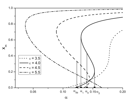
Figure 5: Phase and bifurcation diagrams for non-equilibrium transitions at $\tau_{J}=0.3$: a) phase diagram in the plane $(\alpha,\varepsilon)$ at pure deterministic case (thin lines) and $\mathcal{M}^{(1)}=0.1$, 0.5 (thick lines); b) most probably stationary values $x_{m}$ versus $\alpha$ at different $\varepsilon$ and $\mathcal{M}^{(1)}=0.1$. Domains $I$ and $III$ correspond to diluted and dense states, respectively; in the domain $II$ both states are possible.

Dashed lines in Fig.5a correspond to coexistence of two phases: equivalence of two minima of the function $V(x)=-\int{\rm d}x^{\prime}f(x^{\prime})$ (thin line) and $U_{ef}(x)$ (thick line). The dash-dotted lines starting at the point $B$ relate to the system parameters where the minimum of $U_{ef}$ at $x=x_{m}$ equals $U_{ef}(x=b_{0})$, where $b_{0}=0$ is the lower natural boundary of the diffusion process $x(t)$. From the mathematical viewpoint at such choice of the system parameters one has a unique minimum at $x=x_{m}$, but due to existence of boundary $b_{0}$ one has an “effective minimum” of $U_{ef}$ at $x=b_{0}$. This minimum relates to the probability density of the adsorbate absence. Therefore, the dash-dotted lines mean an equivalence of both the absence of the adsorbate and the existence of the dense state with $x_{m}\neq 0$. The dotted line denotes values for $\varepsilon$ and $\alpha$ at which $x_{m}$ takes zeroth values and belongs to the boundary $b_{0}$. At large noise intensity ($\mathcal{M}^{(1)}=0.5$) the dash-dot-dot line starting at the point $C$ denotes equivalence of two “effective” minima of $U_{ef}$ at $x=b_{0}$ and at $x=b_{1}$, where $b_{1}=1$ is the upper boundary of the diffusion process. Therefore, the dash-dot-dot line corresponds to equivalence of both states absence of the adsorbate and pure dense state. From Fig.5a it follows that the colored noise results in a decrease of the critical values for the system parameters $\alpha$ and $\varepsilon$ (cf. cases of white and colored noise influence when $\mathcal{M}^{(1)}=0$ and $\mathcal{M}^{(1)}\neq 0$, respectively). Therefore, if the system is subjected to the colored noise, then non-equilibrium unimodal/bimodal transitions are possible at lower lateral interaction energies $\varepsilon$ and adsorption rates $\alpha$. Bifurcation diagram illustrating stationary values $x_{m}$ versus the adsorption rate $\alpha$ is shown in Fig.5b. Here for the solid line quantities $\alpha_{1}$ and $\alpha_{2}$ belong to spinodals (solid lines in Fig.5a); $\alpha_{0}$ corresponds to the coexistence line; $\alpha_{0b}$ (see dashed line) relates to the coexistence line of two states $x_{m}\neq 0$ and $x_{m}=b_{0}$.

6 Analysis of stationary patterns

The extreme of $\mathcal{U}_{ef}[x]$ relates to the stationary patterns $x_{st}$ which can be computed setting the first variation of $\mathcal{U}_{ef}[x]$ with respect to $x$ equal to zero, i.e. $\delta\mathcal{U}_{ef}[x]=0$. From Eq.(44) it follows that stationary patterns can be obtained as solutions of the problem

$$f(x)+D_{0}\nabla\cdot[\nabla x-G(x)\nabla\mathcal{L}_{SH}x]-\frac{c_{0}\tau_{J}\mathcal{M}^{(1)}}{2}f^{\prime\prime}(x)=0.$$ (45)

In order to study stability of possible solution in the vicinity of the fixed point $x_{m}$ related to extrema positions of the homogeneous distribution we assume $x(r)-x_{m}\propto\exp({\rm i}\varkappa r)$, where $\varkappa$ can have real and imaginary parts responsible for spatial modulations and stability of the solution, respectively. After linearization of Eq.(45) one has

$$D_{0}\varkappa^{2}(1-G(x_{m})[q_{0}^{2}-\varkappa^{2}]^{2})=f^{\prime}(x_{m})-\frac{\tau_{J}\tau_{c}\sigma^{2}}{2}f^{\prime\prime\prime}(x_{m}),$$ (46)

where we put $c_{0}=1$, $\mathcal{M}^{(1)}=\tau_{c}\sigma^{2}$.

According to obtained values for $\varkappa$ from Eq.(46) we have computed a stability diagram shown in Fig.6a for both stochastic system with $\mathcal{M}^{(1)}=0.1$ and deterministic one. It is seen that in the case of the noiseless system there is unique line of a hyperbolic form dividing domains of unstable $(U)$ an stable $(S)$ patterns (see thin line). At large $\varepsilon$ it tends to the axis $\alpha=0$. It follows that increasing the lateral interaction energy or the adsorption rate independently one can induce formation of stable stationary patterns. If colored fluctuations ($\mathcal{M}^{(1)}\neq 0$) are not negligibly small, then the picture of stationary pattern formation can be changed crucially. Here the thick curve dividing domains of stable and unstable stationary solutions at large $\varepsilon$ tends to the dependence $\varepsilon(\alpha)$ denoting formation of the first nonzero $x_{m}$ (line (OB) in Fig.5a). It follows that as lateral interaction energy increases at fixed small values for adsorption rate one can move from unstable domain into domain of stable stationary patterns. At further increase in $\varepsilon$ we move again into domain of unstable solutions. Therefore, a some kind of re-entrant pattern-forming transition is realized. Starting from domain of unstable stationary patterns at elevated values for $\alpha$ we move into the domain of stable stationary solutions. Continuing an increase in $\varepsilon$ we get a re-entrantce, where unstable stationary patterns can be observed. The corresponding part of the stability diagram denoting re-entrant formation of unstable stationary patterns (a “beak”) is a part of phase diagram describing noise-induced transitions (see Fig.5a). At further increase in $\varepsilon$ one can move again from domain of stable stationary patterns into domain of unstable stationary patterns. Finally, at large $\alpha$ the re-entrant ordering (formation of stable stationary patterns) can be observed. One dimensional stationary patterns are shown in Fig.6b where $L_{max}$ is the maximal period for one from three patterns obtained at $\alpha$ and $\varepsilon$ related to coordinates of points $A$, $B$ and $C$ in Fig.6a. It is seen that at small $\alpha$ one should expect a formation of islands of adsorbate. Such situation is possible for deposition of molecules (polymers). At large $\alpha$ relevant for deposition of atoms on metal surface islands of diluted phase (vacancy islands) can be organized.

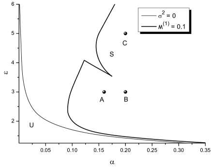
a) b)

Figure 6: (a) Stability diagram for stationary patterns: $U$ and $S$ denote domains of unstable and stable patterns. (b) Profiles of stationary patterns related to points $A(\alpha=0.14,\varepsilon=3.0)$, $B(\alpha=0.2,\varepsilon=3.0)$ and $C(\alpha=0.2,\varepsilon=5.0)$ in plot (a) at $D_{0}=3.0$, $\mathcal{M}^{(1)}=0.1$.

7 Quasi-stationary limit

Let us consider evolution of islands of adsorbate or vacancies (inclusions) having radius $R$ taking into account that the most probable state $x_{m}$ is reached and the system fluctuates around it. We assume $(x_{m}-x_{\infty})\leq x_{m}$ where $x_{\infty}$ plays a role of thermodynamics concentration value, in other words a supersaturation is small.

Let us introduce a quantity $y\equiv x_{m}-x_{R}$ measuring a deviation of the inclusion form from a sphere of the radius $R$. Using the standard approach [45] one can assume the concentration in the vicinity of a spherical inclusion as follows: $x_{R}=x_{\infty}(1+R_{s}/R)$, $R_{s}=2\nu\Omega/T$ is determined trough the surface tension $\nu$, atomic volume $\Omega$ and temperature $T$. Then, the diffusion flux $j(y)$ in the vicinity of the inclusion coincides with velocity of its radius change: ${\rm d}R/{\rm d}t=j(y)$. Using the standard formalism of the coalescence theory [45], we can replace the derivative operator $\nabla$ in the flux $j(y)=D_{0}\nabla(1-G(x_{m})\nabla\mathcal{L}_{SH}(q_{0},\nabla))y$ by $R^{-1}$. As a result we obtain an evolution equation for the radius of inclusion in the form

$$\frac{{\rm d}R}{{\rm d}t^{\prime}}=\frac{1}{R}\left(1-\frac{G(x_{m})}{R}\mathcal{L}_{SH}(q,R^{-1})\right)\left[\frac{1}{R_{c}}-\frac{1}{R}\right],$$ (47)

where $t^{\prime}\equiv tD_{0}\Sigma$, $\Sigma\equiv 2\nu\Omega x_{\infty}/T$, $\Delta\equiv x_{m}-x_{\infty}\geq 0$ plays the role of a supersaturation, $R_{c}\equiv\Sigma/\Delta>0$ is the critical radius of the inclusion, $\mathcal{L}_{SH}(q,R^{-1})\equiv\left(q^{2}+{R}^{-2}\right)^{2}$; next we drop prime for the time variable. Equation (47) can be rewritten in the form $\dot{R}=-{{\rm d}W}/{\rm d}R$, where a potential $W(R)$ can be used in a further study.

At first let us consider the simplest case of $\Delta=const$ where the critical radius $R_{c}$ remains constant. In the stationary case we put $\dot{R}=0$ in Eq.(47). Such assumption relates to autonomous regime of islands formations. As far as $\Delta\sim 10^{-2}$ the critical radius is large but finite. One of the stationary solution having physical meaning is $R_{0}=L$, where $L\to\infty$ is the thermodynamic limit of the system size. There is another solution $R_{0}$ responsible for formation of stationary patterns characterized by $\Re\varkappa(\alpha,\varepsilon,\mathcal{M}^{(1)})\neq 0$. It can be computed from the condition $R_{0}^{5}=G(x_{m})(1+q^{2}R_{0}^{2})^{2}$. The corresponding dependencies $R_{0}(\alpha)$ at $R_{0}<R_{c}$ at different $\varepsilon$ and $\mathcal{M}^{(1)}$ are shown in Fig.7a. Its values are bounded by stability criteria $\Im\varkappa(\alpha,\varepsilon,\mathcal{M}^{(1)})\leq 0$. It follows that $R_{0}$ relate to large stable values for $x_{m}$. Using the potential $W(R)$ one can find that $W(R)$ has two asymptotics: $W(R\to 0)\to\infty$, $W(R\to\infty)\to-\infty$. Therefore, the quantity $R_{c}$ corresponds to a maximum of $W$, whereas $R_{0}$ defines its minimum position. Hence, at $R>R_{c}$ all previously organized inclusions at early stages start to grow; contrary, at $R<R_{c}$ the corresponding patterns relax to spherical inclusions having fixed radius $R_{0}$. In order to illustrate the corresponding time dependencies of the inclusion radius we solve numerically Eq.(47) (see Fig.7b).

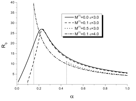
a) b)

Figure 7: Stationary values for $R_{0}$ at different values for $\varepsilon$ and $\mathcal{M}^{(1)}$ (plot (a)) and typical dependencies $R(t)$ at different initial conditions and at $\alpha=0.6$, $\varepsilon=3$, $\mathcal{M}^{(1)}=0.5$ (plot (b)). Other parameters are: $D_{0}=3.0$, $\tau_{J}=0.3$, $\Delta=10^{-2}$.

As far as $R_{0}$ has unique dependence versus the system parameters, one can solve Eq.(47) analytically rewriting it for the quantity $\rho\equiv R/R_{c}$ in the form $\rho^{3}\dot{\rho}=(\rho-\rho_{0})(\rho-1)$, where $\rho_{0}\equiv R_{0}/R_{c}$, time derivative are taken with respect to $t^{\prime}\equiv t/R_{c}^{3}$ (next we drop prime for the time variable). Dividing variables, from the formal solution of Eq.(47) following asymptotics can be found: in the vicinity of $\rho=\rho_{c}\equiv 1$ there are exponentially increasing deviations from the critical radius; in the vicinity of $\rho_{0}$ the exponential decaying $\rho(t)$ is observed.

Let us analyze the system behavior considering time dependence of the supersaturation $\Delta(t)>0$. Hence there is a time dependent variable $R_{c}(t)$. Next it will be convenient to move to new variables: $z(t)\equiv R_{c}(t)/R_{c}(0)$, $u(t)\equiv R(t)/R_{c}(t)$. As a new time variable we introduce $\tau=4\ln z$. It yields the derivative ${\rm d}u^{4}/{\rm d}\tau=-u^{4}+\gamma(\tau)R^{3}{\rm d}R/{\rm d}t$, where $\gamma(\tau)=(R_{c}^{4}(0)z^{3}{\rm d}z/{\rm d}t)^{-1}$. Using Eq.(47) and taking into account that there is unique value $R_{0}$, one has $R^{3}{\rm d}R/{\rm d}t=(R-R_{0})(R/R_{c}-1)$. Therefore, an equation for the variable $u$ takes the form

$$\frac{{\rm d}u^{4}}{{\rm d}\tau}=-u^{4}-R_{0}\gamma(u-1)+\gamma R_{c}u(u-1).$$ (48)

Let us estimate time asymptotics for both $R(t)$ and $R_{c}(t)$. To this end we consider the limit $\tau\gg 1$. It allows one to put ${\rm d}u^{4}/{\rm d}\tau=0$ or $u^{4}=-R_{0}\gamma(u-1)+\gamma R_{c}u(u-1)$. As far as the term in the left hand side has no time dependent coefficient and $u(\tau\to\infty)=const$ it means that all coefficients in the right hand side should be constants at $\tau\to\infty$. When we assume $\gamma(\tau\to\infty)=const$ the coefficient $\gamma R_{c}$ should take constant value too. Unfortunately, from the definition of $\gamma(\tau)$ we arrive that $R_{c}(t)$ is an increasing function in time leading to non-physical situation where all coefficients from the right hand side of Eq.(48) are constants, not time-dependent functions. Therefore, this assumption fails.

Let us consider another case, setting $\gamma R_{c}=const$ at $\tau\gg 1$. Therefore, from the definition of $\gamma(\tau)$ one can find that $R_{c}(t)\propto t^{1/3}$ and $\gamma(\tau)\to 0$. Therefore, the term $R_{0}\gamma(u-1)$ can be neglected at $\tau\gg 1$. Using the definition of the variable $u$ one can set that the radius of inclusion increases in time according to the Lifshitz-Slyozov law $R(t)\propto t^{1/3}$ [46].

8 Simulations

In order to verify our analytical results we performed numerical simulations by solving the system (19) in $d=2$-dimensional quadratic lattice of the linear size $N=256$ with periodic boundary conditions with the mesh size $\ell=0.5$ and the time step $\Delta t=0.001$. The noise term was modeled as the Ornshtein-Uhlenbeck process [47]. As initial conditions we have used $\langle x(\mathbf{r},0)\rangle=0.5$, $\langle(\delta x)^{2}\rangle=0.1$. All measured quantities were averaged over 15 independent runs.

Typical patterns organized during the system evolution are shown in Fig.8a at $\alpha=0.16$. It is seen that at small times patterns of different sizes are formed. After the system selects patterns with a fixed size. At large time intervals spherical patterns are organized having preferably hexagonal symmetry as the Swift-Hohenberg operator predicts due to elastic interactions [23, 24, 30]. In Fig.8b we plot the corresponding spherically averaged structure function at different times at relevant values for the wave-numbers to show the pattern selecting processes. It is seen that except the main peak related to period of main patterns there are well defined peaks at small wave-numbers (at elevated $k$ the corresponding peaks have very small intensity, not shown here). During the system evolution its intensity decreases and only main peak is realized, its position is shifted toward $\Re\varkappa$ defining the period of stationary patterns. In insertion we have shown structure functions for two cases: $\alpha=0.16$ and $\alpha=0.22$. At $\alpha=0.22$ the period of patterns is smaller as the above stability analysis shows.

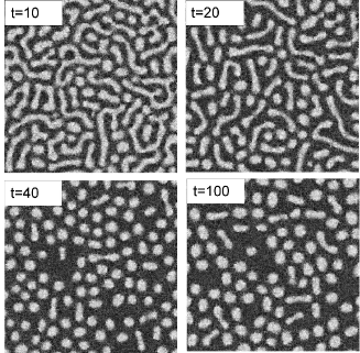
a) b)

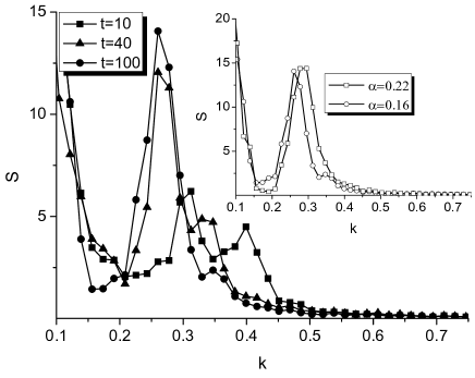
Figure 8: Snapshots of the system evolution (a) and evolution of the spherically averaged structure function (b) at $\alpha=0.16$. Insertion in plot (b) shows structure function at $t=100$ and different values for adsorption rate. Other parameters are: $D_{0}=3.0$, $\tau_{J}=0.3$, $\mathcal{M}^{(1)}=0.1$.

Considering quasi-stationary limit (time intervals where $\langle x\rangle$, $\langle(x-\langle x\rangle)^{2}\rangle$ and $\langle(x-\langle x\rangle)^{3}\rangle$ are time-independent quantities, $t\sim 10^{2}$) we can compute radius of inclusions by measuring surfaces of islands (number of points belonging to islands having spherical form). Evolution of the number of inclusion having fixed radius $R$ at different $\alpha$ are shown in Fig.9. It is seen that during the system evolution a distribution of islands becomes more compact and it has one the most probable value for $R$.

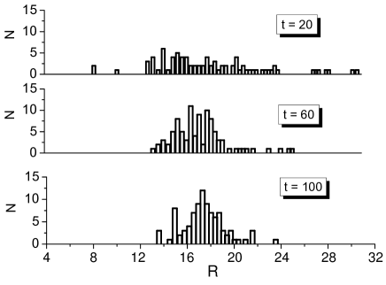
a) b)

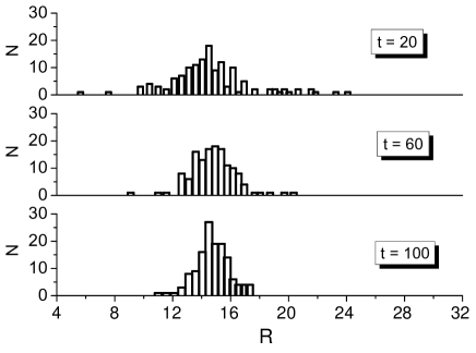
Figure 9: Number of islands $N$ versus the island size $R$ at different times. Plots (a) and (b) relate to $\alpha=0.16$ and $\alpha=0.3$ Other parameters are: $D_{0}=3.0$, $\tau_{J}=0.3$, $\mathcal{M}^{(1)}=0.1$.

After averaging this radius over independent runs we obtain the dependencies of the optimal characteristic length $\langle R_{opt}\rangle(\alpha)$ shown in Fig.10, where $\langle\cdots\rangle$ means average over experiments. On the top we present snapshots of patterns realized at different values for $\alpha$ at fixed $\varepsilon$. It is well seen that graphs $\langle R_{opt}\rangle(\alpha)$ repeat analytical dependencies $R_{0}(\alpha)$ in Fig.7a at small and large $\alpha$ where spherical islands forming hexagonal crystal structure are possible. At intermediate values for $\alpha$ strip patterns are realized and no spherical islands are possible. Therefore, in Fig.10 there are gaps related to domains for $\alpha$ where no spherical islands are realized . Fitting procedure allows us to find that at small $\alpha$ where inclusions of the dense phase are possible the exponential law is realized, $A-\langle R_{opt}\rangle=B^{\alpha}$, where $A$ and $B$ are fitting parameters. At large $\alpha$ when islands of vacancies are realized one has exponential decaying, $\langle R_{opt}\rangle-A=\exp(-\alpha/B)$. Therefore, an introduction of the Swift-Hohenberg operator into the model for the system dynamics allows one to describe formation of lattice with different kind of inclusions: at small $\alpha$ one has molecular/atom inclusions forming hexagonal lattice, at large $\alpha$ one has a situation when deposition of atoms on metal surface can be described with formation of lattice of vacancy islands.

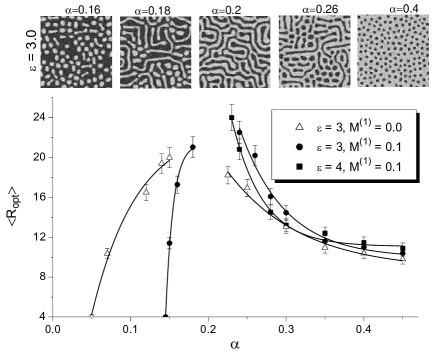
Figure 10: Averaged linear size of islands versus adsorption rate $\alpha$ at different $\varepsilon$ and $\mathcal{M}^{(1)}$. Stationary patterns observed at $\varepsilon=0.3$ at different $\alpha$ are shown on the top. Other parameters are: $D_{0}=3.0$, $\tau_{J}=0.3$.

To estimate the spatial size of patterns one can consider typical limits of $r_{0}\sim 1nm$ and $L_{dif}\sim 1\mu m$. For the system of deposition of Al on TiN (100) the estimation in Ref.[14] shows that at room temperature with the lattice constant $a_{Al}=4.05\times 10^{-10}m$ and pair interaction energy $\varepsilon=-0.22eV$ with lattice coordination number $Z=4$ the size of patterns with $\mu=Za^{2}_{Al}\varepsilon/T$ is around $30\times 10^{-9}$m. Therefore, patterns such as inclusions of dense/diluted phase are of nano-scales and are nano-patterns [15]. Patterns of diluted phase usually are realized as lattice of vacancy islands (for example in absorbed monoatomic layer of Ag deposited on Ru(0001) Ref.[7]).

9 Conclusions

We have studied pattern formation processes in stochastic reaction-diffusion systems with the relaxation flux obeying Maxwell-Cattaneo equation. The novelty of our approach is the usage of the phase field crystals formalism with special geometry of realized patterns and introduction of multiplicative noise obeying fluctuation-dissipation relation.

Pattern formation is discussed on the model system describing adsorption-desorption processes. Considering pattern formation at early stages of the system evolution we have analyzed temporal stability of patterns and have shown that pattern selection processes are realized as a result of the diffusion flux relaxation to its stationary value.

To study stationary patterns we have obtained the effective Fokker-Planck equation and its stationary solution. It was shown that multiplicative noise can induce non-equilibrium transitions at low energies for the adsorbate interactions. Using stability analysis we have computed diagram illustrating domains of the system parameters where stationary patterns can be realized. It was shown that introduced multiplicative noise can induce re-entrant pattern-forming transitions where stable/unstable stationary patterns exist inside fixed intervals for lateral interaction energy of the adsorbate. Stationary patterns organized during the system evolution form the crystalline structure of hexagonal symmetry. It is explained by introduction of the Swift-Hohenberg operator into the expansion for the interaction potential for the adsorbate.

Considering quasi-stationary limit we have discussed evolution of radius of the dense phase inclusions into diluted one or vice versa. Using this alternative approach related to coalescence theory it was shown that all patterns are described by the characteristic radius $R_{0}$ that less then the critical one $R_{c}$. In the vicinity of $R_{c}$ spatial perturbations grow exponentially, whereas in the vicinity of $R_{0}$ such perturbations exponentially decay. We have found that both critical and characteristic radii have time asymptotics related to the Lifshits-Slyozov law.

References

- [1] T.Zambelli, J.Trost, J.Wintterlin, G.Ertl, Phys.rev.Lett., 79, 795 (1996)
- [2] V.Gorodetskii, J.Lauterbach, H.A.Rotermund, J.H.Block, G.Ertl, Nature, 370, 276 (1994)
- [3] K.Kern, H.Niehus, A.Schatz, P.Zeppenfeld, J.George, G.Cosma, Phys.Rev.Lett, 67, 855 (1991)
- [4] T.M.Parker, L.K.Wilson, N.G.Condon, F.M.Leissle, Phys.Rev.B, 56, 6458 (1997)
- [5] H.Brune, M.Giovannini, K.Bromann, K.Kern, Nature, 394, 451 (1998)
- [6] P.G.Clark, C.M.Friend, J.Chem.Phys., 111, 6991 (1999)
- [7] K.Pohl, M.C.Bartelt, J.de la Figuera, N.C.Bartelt, J.Hrbek, R.Q.Hwang, Nature 397, 238 (1999)
- [8] P.Zepenfeld, M.Krzyzowski, C.Romainczyk, G.Gomsa, M.G.Lagally, Phys.Rev.Lett., 72, 2737 (1994)
- [9] V.I.Marchenko, JETP Lett., 67, 855 (1991)
- [10] D.Vanderbit, Surf.Sci., 268, L300 (1992)
- [11] A.Mikhailov, G.Ertl, Chem.Phys.Lett., 238, 104 (1994)
- [12] D.Batogkh, M.Hildebrant, F.Krischer, A.Mikhailov, Phys.Rep., 288, 435 (1997)
- [13] Sergio E.Mangioni, Horacio S. Wio, Phys.Rev.E., 71, 056203 (2005)
- [14] M.G.Clerc, E.Tirapegui, M.Trejo, Phys.Rev.Lett., 97, 176102 (2006)
- [15] M.G.Clerc, E.Tirapegui, M.Trejo, Eur.Phys.J. ST. 146, 407 (2007)
- [16] Sergio E.Mangioni, Physica A, 389, 1799 (2010)
- [17] D.O.Kharchenko, S.V.Kokhan, A.V.Dvornichenko, Physica D, 238, 2251 (2009)
- [18] M.Ibanes, J.Garcia-Ojalvo, R.Toral, J.M.Sancho, Phys.Rev.Lett., 87, 020601, (2001).
- [19] F.J.Cao, K.Wood, K.Lindenberg, Phys.Rev.E,76, 051111 (2007)
- [20] O.Carriollo, M.Ibanes, J.Garcia-Ojalvo, J.Casademunt, J.M.Sancho, Phys.Rev.E, 67, 046110 (2003)
- [21] J.Buceta, K.Lindenberg, Phys.Rev.E, 69, 011102 (2004)
- [22] D.O.Kharchenko, A.V.Dvornichenko, Eur.Phys.J.B 61, 95 (2008).
- [23] K.R.Elder, Mark Katakowski, Mikko Haataja, Martin Grant, Phys.Rev.Lett., 88, 245701 (2002)
- [24] K.R.Elder, Martin Grant, Phys.Rev.E., 70, 051605 (2004)
- [25] K.R.Elder, Nikolas Provatas, Joel Berry, Peter Stefanovich, Martin Grant, Phys.Rev.B, 75, 064107 (2007).
- [26] P.F.Tupper, M.Grant, EPL, 81, 40007 (2008)
- [27] D.D.Joseph, L.Preziosi, Rev.Mod.Phys., 61, 41 (1989)
- [28] Werner Horsthemke, Phys.Rev.E, 60, 2651 (1999)
- [29] J.A.P.Ramos, E.Granato, S.C.Ying, C.V.Achim, K.R.Elder, T.Ala-Nissila, Phys.Rev.E, 81, 011121 (2010)
- [30] Peter Stafanovich, Mikko Haataja, Nikolas Provatas, Phys.Rev.Lett., 96, 225504 (2006)
- [31] D.Kharchenko, I.Lysenko, V.Kharchenko, Physica A, 389, 3356 (2010)
- [32] Dmytro Kharchenko, Vasyl Kharchenko, Irina Lysenko, Cent.Eur.J.Phys., doi:10.2478/s11534-010-0076-y
- [33] M.Heldebrand, A.S.Mikhailov, G.Ertl, Phys.Rev.Lett., 81, 2602(4) (1998)
- [34] M.Heldebrand, A.S.Mikhailov, G.Ertl, Phys.Rev.E, 58, 5483(11) (1998)
- [35] S.B.Casal, H.S.Wio, S.Mangioni, Physica A, 311, 443 (2002)
- [36] Umberto Marini Bettolo Marconi, Andrea Puglisi, Lamberto Rondoni, Angelo Vulpiani, Phys.Rep., 461, 111 (2008)
- [37] C.W.Gardiner, Handbook of Stochastic Methods, (Springer, New York, 1989).
- [38] P.Hanggi, P.Jung, Adv.Chem.Phys., 89, 239 (1995)
- [39] E.A.Novikov, Sov.Phys.JETP, 20, 1290 (1965)
- [40] P.K.Galenko, Dmitrii Kharchenko, Irina Lysenko, Physica A, 389, 3443 (2010)
- [41] N.G.Van Kampen, Stochastic Processes in Physics and Chemistry (North–Holland, Amsterdam, 1992).
- [42] V.E.Shapiro, Phys.Rev.E. 48, 109 (1993)
- [43] A.I.Olemskoi, D.O.Kharchenko, I.A.Knyaz’, Phys.Rev.E, 71, 041101 (2005)
- [44] D.O.Kharchenko, I.A.Knyaz’, Eur.Phys.J.B, 32, 375 (2003)
- [45] L.P. Pitaevskii, E.M. Lifshitz, Physical Kinetics, Vol. 10 (1st ed.) (Pergamon Press, 1981)
- [46] I.M.Lifshitz, V.V.Slyozov, J.Phys.Chem.Solids 19, 35 (1961).
- [47] J.Garcia–Ojalvo, J.M.Sancho, Noise in Spatially Extended Systems (Springer–Verlag, New York, 1999).