Curve Crossing Problem with Arbitrary Coupling: Analytically Solvable Model

Abstract

We give a general method for finding an exact analytical solution for the two state curve crossing problem. The solution requires the knowledge of the Green’s function for the motion on the uncoupled potential. We use the method to find the solution of the problem in the case of parabolic potentials coupled by Gaussian interaction. Our method is applied to this model system to calculate the effect of curve crossing on electronic absorption spectrum and resonance Raman excitation profile.

I Introduction

Nonadiabatic transition due to potential curve (or surface) crossing is one of the most important mechanisms to effectively induce electronic transitions in collisions Naka1 ; Niki ; Child ; Osherov ; Nikitin ; Nakamura ; Naka2 ; Shaik ; Imanishi ; Thiel ; Yoshimori ; Engleman ; Mataga ; Dev . Two state curve crossing can be classified into the following two cases according to the crossing scheme: (1) Landau-Zener (L.Z) case, in which the two diabatic potential curves have the same signs for the slopes and (2) non-adiabatic tunnelling (N.T) case, in which the diabatic curves have the opposite sign for slopes. There is also a non-crossing non-adiabatic transition called the Rosen-Zener-Demkov type Naka1 ; Naka2 , in which two adiabatic potentials are in near resonance at large $R$. The theory of non-adiabatic transitions dates back to $1932$, when the works for curve-crossing and non-crossing were published by Landau Landau , Zener Zener and Stueckelberg Stueckelberg and by Rosen and Zener Rosen respectively. Two categories might be classified for finding an exact analytical solution of the curve crossing problem. The first is that an exact analytical solution can be obtained for the whole region of the variable (say $x$ here, see in the next section). For example, Osherov and Voronin solved the case where two diabatic potentials are constant with exponential coupling Voronin . C. Zhu solved the case where two diabatic potentials are exponential with exponential coupling Nikitinmodel . In our earlier publications we have reported the analytical solution in the case, where two or more arbitrary potentials are coupled by Dirac Delta interactions Ani1 ; AniThesis ; Ani2 ; AniBook ; Ani3 ; Ani4 . The second is that an exact analytical solution is only possible for the asymptotic region. Then, physical quantities such as eigenvalues, scattering matrices can still be solved in an exact analytical form, providing that the connection problem of the asymptotic solution is known. The Stokes phenomenon Stokes of asymptotic solution of the ordinary differential equation provides a powerful tool to deal with these kinds of problems Heading ; Hinton ; Zhu . Generalizing the real variable to the complex variable and tracing the asymptotic solution around the complex plane, the connection matrix which connects the asymptotic solution in the complex plane can be expressed in terms of Stokes constants. Recent work by Zhu and Nakamura Zhu found an exact analytical solution of the Stokes constants for the second-order ordinary differential equation with the coefficient function as the fourth-order polynomial. In this way, exact analytical solutions of scattering matrices were obtained for the two state linear curve crossing problem with constant coupling Aquilanti .

II The model

We consider two diabatic curves, crossing each other. There is a coupling between the two curves, which causes transitions from one curve to another. This transition would occur approximately in the vicinity of the crossing point. In particular, it will occur in a narrow range of $x$, given by

$$\left|V_{1}(x)-V_{2}(x)\right|\simeq\left|V(x_{c})\right|.$$ (1)

where $x$ denotes the nuclear coordinate and $x_{c}$ is the crossing point. $V_{1}$ and $V_{2}$ are the diabatic curves and $V$ represent the coupling between them. Therefore it is interesting to analyze a model, where coupling is localized in space near $x_{j}$ given by $V(x)=k_{j}\delta(x-x_{j})$, where $k_{j}$ is the coupling strength Ani1 ; AniThesis ; AniBook . The majority of the problems of interest, however do not corresponds to a localized coupling and one requires different forms of coupling $V(x)$ for proper description of dynamics in different cases. We express the arbitrary coupling function $V(x)$ in terms of a linear combination of Dirac Delta functions SKG ; Szabo . Expressing the arbitrary coupling function $V(x)$ in terms of Dirac Delta functions has the advantage that it can be solved exactly by using analytical methods Ani1 ; AniThesis ; Ani2 ; AniBook ; Ani3 ; Ani4 . An arbitrary coupling $V(x)$ can be written as

$$V(x)=\int_{-\infty}^{\infty}dx^{\prime}V(x^{\prime})\delta(x-x^{\prime})$$ (2)

and the above integral can be discritized as

$$V(x)=\sum_{j=1}^{N}k_{j}\delta(x-x_{j}),$$ (3)

here $k_{j}$ are constants, given by

$$k_{j}=w_{j}V(x_{j}).$$ (4)

The weight factor $w_{j}$ varies depending on the scheme of discritization used SKG .

III Exact analytical solution

We start with a particle moving on any of the two diabatic curves. The problem is to calculate the probability that the particle will still be on any one of the diabatic curves after a time $t$. We write the probability amplitude as

$$\Psi(x,t)=\left(\begin{array}[]{c}\psi_{1}(x,t)\\ \psi_{2}(x,t)\end{array}\right),$$ (5)

where $\psi_{1}(x,t)$ and $\psi_{2}(x,t)$ are the probability amplitude for the two states. $\Psi(x,t)$ obey the time dependent Schr$\stackrel{{\scriptstyle..}}{{o}}$ dinger equation (we take $\hbar=1$ here and in subsequent calculations)

$$i\frac{\partial\Psi(x,t)}{\partial t}=H\Psi(x,t),$$ (6)

where $H$ is defined by

$$H=\left(\begin{array}[]{cc}H_{1}(x)&V(x)\\ V(x)&H_{2}(x)\end{array}\right),$$ (7)

where $H_{i}(x)$ is

$$H_{i}(x)=-\frac{1}{2m}\frac{\partial^{2}}{\partial x^{2}}+V_{i}(x).$$ (8)

We find it convenient to define the half Fourier Transform $\overline{\Psi}(E)$ of $\Psi(t)$ by

$$\overline{\Psi}(E)=\int_{0}^{\infty}\Psi(t)e^{iEt}dt.$$ (9)

Half Fourier transformation of Eq. (6) leads to

$$\left(\begin{array}[]{c}\overline{\psi}_{1}(E)\\ \overline{\psi}_{2}(E)\end{array}\right)=i\left(\begin{array}[]{cc}E-H_{1}&-V\\ -V&E-H_{2}\end{array}\right)^{-1}\left(\begin{array}[]{c}\psi_{1}(0)\\ \psi_{2}(0)\end{array}\right).$$ (10)

This may be written as

$$\overline{\Psi}(E)=iG(E)\Psi(0).$$ (11)

$G(E)$ is defined by $(E-H)$ $G(E)=I$. In the position representation, the above equation may be written as

$$\overline{\Psi}(x,E)=i\int_{-\infty}^{\infty}G(x,x_{0};E)\overline{\Psi}(x_{0},E)dx_{0},$$ (12)

where $G(x,x_{0};E)$ is

$$G(x,x_{0};E)=\langle x|(E-H)^{-1}|x_{0}\rangle.$$ (13)

Writing

$$G(x,x_{0};E)=\left(\begin{array}[]{cc}G_{11}(x,x_{0};E)&G_{12}(x,x_{0};E)\\ G_{21}(x,x_{0};E)&G_{22}(x,x_{0};E)\end{array}\right)\begin{array}[]{cc}&\\ &\end{array}$$ (14)

and using the partitioning technique Lowdin we can write

$$G_{11}(x,x_{0};E)=\langle x|[E-H_{1}-V(E-H_{2})^{-1}V]^{-1}|x_{0}\rangle.$$ (15)

The above equation is true for any general $V$. This expression simplify considerably if $V$ is expressed as a sum of delta functions SKG ; Szabo . In that case $V$ may be written as $V=\sum_{j=1}^{N}K_{j}S_{j}=\sum_{j=1}^{N}K_{j}|x_{j}\rangle\langle x_{j}|$. Then

$$G_{11}(x,x_{0};E)=\langle x|[E-H_{1}-\sum_{j=1}^{N}K_{j}^{2}G_{2}^{0}(x_{j},x_{j};E)S_{j}]^{-1}|x_{0}\rangle,$$ (16)

where

$$G_{2}^{0}(x,x_{0};E)=\langle x|(E-H_{2})^{-1}|x_{0}\rangle,$$ (17)

and corresponds to propagation of the particle starting at $x_{0}$ on the second diabatic curve, in the absence of coupling to the first diabatic curve. Now we use the operator identity Sebastian ; Sebas

$$(E-H_{1}-\sum_{j=1}^{N}K_{j}^{2}G_{2}^{0}(x_{j},x_{j};E)S_{j})^{-1}=(E-H_{1})^{-1}+(E-H_{1})^{-1}\sum_{j=1}^{N}K_{j}^{2}G_{2}^{0}(x_{j},x_{j};E)S_{j}[E-H_{1}-\sum_{j=1}^{N}K_{j}^{2}G_{2}^{0}(x_{j},x_{j};E)S_{j}]^{-1}.$$ (18)

Inserting the resolution of identity $I=\int_{-\infty}^{\infty}dy$ $|y\rangle$ $\langle y|$ in the second term of the above equation, we arrive at

$$G_{11}(x,x_{0};E)= G_{1}^{0}(x,x_{0};E)+\sum_{j=1}^{N}K_{j}^{2}G_{1}^{0}(x,x_{j};E)$$ (19)

$$\times G_{2}^{0}(x_{j},x_{j};E)G_{11}(x_{j},x_{0};E).$$

Considering the above equation at the discrete points $x_{i}$, we obtain a set of linear equations, which can be written as

$$AP=Q,$$ (20)

where the elements of the matrices $A=[a_{ij}]$, $P=[p_{i}]$ and $Q=[q_{i}]$ are given by

$$a_{ij}=-k_{i}^{2}G^{0}_{1}(x_{i},x_{j};E)G^{0}_{2}(x_{j},x_{j};E)+\delta_{ij}$$ (21)

$$p_{i}=G_{11}(x_{i},x_{0};E)$$

$$q_{i}=G^{0}_{1}(x_{i},x_{0};E)$$

One can solve the matrix equation i.e. Eq. (20) easily and obtain $G_{11}(x_{i},x_{0};E)$ for all $x_{i}$. Eq. (19) then yield $G_{11}(x,x_{0};E)$. Similar one can derive expressions for $G_{12}(x,x_{0};E)$, $G_{22}(x,x_{0};E)$ and $G_{21}(x,x_{0};E)$. Using these expressions for the Green’s function in Eq. (11) we can calculate $\overline{\Psi}(E)$ explicitely. The expressions that we have obtained for $\overline{\Psi}(E)$ are quite general and are valid for any $V_{1}(x)$ and $V_{2}(x)$.

IV Electronic Absorption Spectra and Resonance Raman Excitation Profile

In this section we apply the method to the problem involving harmonic potentials. We consider a system of three potential energy curves, ground electronic state and two ‘crossing’ excited electronic states (electronic transition to one of them is assumed to be dipole forbidden and while it is allowed to the other) Zink ; ZinkPRL . We calculate the effect of ‘crossing’ on electronic absorption spectra and on resonance Raman excitation profile. The propagating wave functions on the excited state potential energy curves are given by solution of the time dependent Schrödinger equation

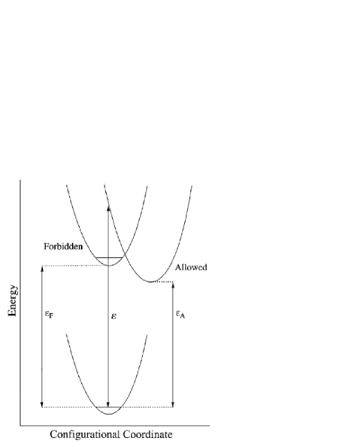
Figure 1: Schematic diabatic potential energy curves that illustrate the model. The forbidden state is labeled F ; the allowed state is labeled A .

$$i\frac{\partial}{\partial t}\left(\begin{array}[]{c}\psi_{1}^{vib}(x,t)\\ \psi_{2}^{vib}(x,t)\end{array}\right)=\left(\begin{array}[]{cc}H_{vib,e1}(x)&V_{12}(x)\\ V_{21}(x)&H_{vib,e2}(x)\end{array}\right)\left(\begin{array}[]{c}\psi_{1}^{vib}(x,t)\\ \psi_{2}^{vib}(x,t)\end{array}\right).$$ (22)

In the above equation $H_{vib,e1}(x)$ and $H_{vib,e2}(x)$ describes the vibrational motion of the system in the first electronic excited state (allowed) and second electronic excited state (forbidden) respectively

$$H_{vib,e1}(x)=-\frac{1}{2m}\frac{\partial^{2}}{\partial x^{2}}+\frac{1}{2}mE_{A}^{2}(x-a)^{2}$$ (23)

and

$$H_{vib,e2}(x)=-\frac{1}{2m}\frac{\partial^{2}}{\partial x^{2}}+\frac{1}{2}mE_{F}^{2}(x-b)^{2}.$$ (24)

In the above $m$ is the oscillator’s mass, $E_{A}$ and $E_{F}$ are the vibrational frequencies on the allowed and forbidden states and $x$ is the vibrational coordinate. Shifts of the vibrational coordinate minimum upon excitation are given by $a$ and $b$, and $V_{12}$ ($V_{21}$) represent coupling between the two harmonic potentials which is taken to be

$$V_{21}(x)=V_{12}(x)=K_{0}e^{-a(x-x_{c})^{2}},$$ (25)

where $K_{0}$ represent the strength of the coupling.

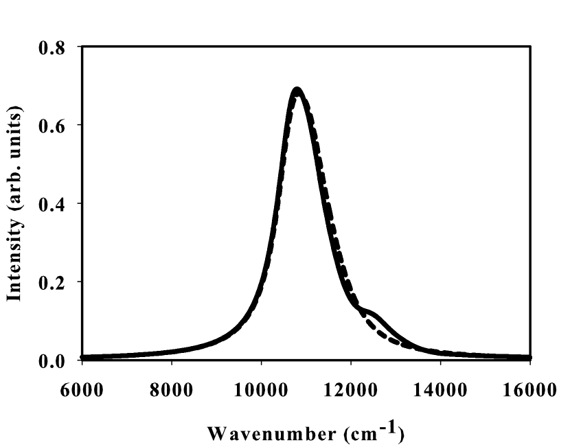
Figure 2: Calculated electronic absorption spectra with coupling (solid line) and without coupling (dashed line). Here the values for the simulations are $E_{0}=E_{A}=E_{F}=400\>cm^{-1}$, $\Gamma=450\>cm^{-1}$, $\varepsilon_{A}=10700\>cm^{-1}$, $\varepsilon_{F}=11500\>cm^{-1}$, $K_{0}=1200\>cm^{-1}$, $a=0.2594\>\AA^{-1}$ and $x_{c}=-0.1991\>\AA$.

The intensity of electronic absorption spectra is given by Zink ; Heller

$$I_{A}(E)\propto Re[\int_{-\infty}^{\infty}dx\int_{-\infty}^{\infty}dx_{0}\Psi_{i}^{vib*}(x)$$ (26)

$$iG(x,x_{0};E+i\Gamma)\Psi_{i}^{vib}(x_{0})],$$

where

$$G(x,x_{0};E+i\Gamma)=\langle x|[(E_{0}/2+E-E_{eg})+i\Gamma-H_{vib,e}]^{-1}|x_{0}\rangle.$$ (27)

and

$$H_{vib,e}=\left(\begin{array}[]{cc}H_{vib,e1}(x)&K_{0}|x_{c}\rangle\langle x_{c}|\\ K_{0}|x_{c}\rangle\langle x_{c}|&H_{vib,e2}(x)\end{array}\right)$$ (28)

Here, $\Gamma$ is a phenomenological damping constant which account for the life time effects. $\Psi_{i}^{vib}(x,0)$ is given by

$$\Psi_{i}^{vib}(x,0)=\left(\begin{array}[]{c}\chi_{i}(x)\\ 0\end{array}\right),$$ (29)

where $\chi_{i}(x)$ is the ground vibrational state of the ground electronic state, $E_{0}$ is the vibrational frequency on the ground electronic state, $\varepsilon_{A}$ is the energy difference between the excited (allowed) and ground electronic state, and for the forbidden electronic state it’s value is $\varepsilon_{F}$. Similarly resonance Raman scattering intensity can be expressed in terms of Green’s function and is given by Heller ; Zink .

$$I_{R}(E)\propto |\int_{-\infty}^{\infty}dx\int_{-\infty}^{\infty}dx_{0}\Psi_{f}^{vib*}(x,0)$$ (30)

$$iG(x,x_{0};E+i\Gamma)\Psi_{i}^{vib}(x_{0},0)|^{2}.$$

In the above $\Psi_{f}^{vib}(x,0)$ is given by

$$\Psi_{f}^{vib}(x,0)=\left(\begin{array}[]{c}\chi_{f}(x)\\ 0\end{array}\right),$$ (31)

where $\chi_{f}(x)$ is the final vibrational state of the ground electronic state. As $G_{i}^{0}(x,x_{0};E)$ for the harmonic potential is known Grosche , we can calculate $G(x,x_{0};E)$. We use Eq. (30) to calculate the effect of curve crossing on resonance Raman excitation profile.

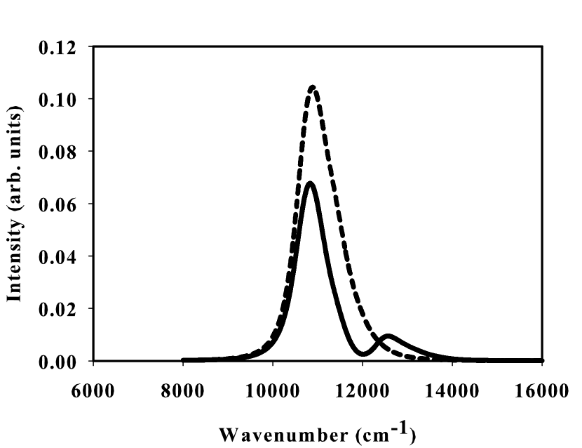
Figure 3: Calculated resonance Raman excitation profile for excitation from the ground vibrational state to the first excited vibrational state, with coupling (solid line) and without coupling (dashed line). Here the values for the simulations are $E_{0}=E_{A}=E_{F}=400\>cm^{-1}$, $\Gamma=450\>cm^{-1}$, $\varepsilon_{A}=10700\>cm^{-1}$, $\varepsilon_{F}=11500\>cm^{-1}$, $K_{0}=1200\>cm^{-1}$, $a=0.2594\>\AA^{-1}$ and $x_{c}=-0.1991\>\AA$.

IV.1 Results using the model

In the following we give results for the effect of curve crossing on electronic absorption spectrum and resonance Raman excitation profile in the case where one dipole allowed electronic state crosses with a dipole forbidden electronic state as in Fig. 1. As in Zink , the ground state curve is taken to be a harmonic potential energy curve with its minimum at zero. The curve is constructed to be representative of the potential energy along a metal-ligand stretching coordinate. We take the mass as $35.4\>amu$ and the vibrational wavenumber as $400\>cm^{-1}$ Zink for the ground state. The first diabatic excited state potential energy curve is displaced by $0.2\>\AA$ and is taken to have a vibrational wavenumber of $400\>cm^{-1}$. Transition to this state is allowed. The minimum of the potential energy curve is taken to be above $10700\>cm^{-1}$ of that of the ground state curve. The second diabatic excited state potential energy curve is taken to be an un-displaced excited state. On that potential energy curve, the vibration is taken to have same wavenumber of $400\>cm^{-1}$. Its minimum is $11500\>cm^{-1}$ above that of the ground state curve. Transition to this state is assumed to be dipole forbidden. The two diabatic curves cross at an energy of $11765\>cm^{-1}$ with $x_{c}=-0.1991\>\AA$. Value of $K_{0}$ we use in our calculation is $K_{0}=1200\>cm^{-1}$ and the value of $a$ we use in our calculation is $a=0.2594\>\AA^{-1}$. The lifetime of both the excited states are taken to be $450\>cm^{-1}$. The calculated electronic absorption spectra is shown in Fig. 2. The profile shown by the dashed line is in the absence of any coupling to the second potential energy curve. The full line has the effect of coupling in it. The calculated resonance Raman excitation profile is shown in Fig. 3. The profile shown by the full line is calculated for the coupled potential energy curves. The profile shown by the dashed line is calculated for the uncoupled potential energy curves. It is seen that curve crossing effect can alter the absorption and Raman excitation profile significantly. However it is the Raman excitation profile that is more effected.

V Conclusions

We have proposed a general method for finding the exact analytical solution for the two state curve crossing problem. Our solution is quite general and is valid for any potentials for which Green’s functions for the motion in the absence of coupling is known. We use the method to find the solution of the problem in the case of parabolic potentials coupled by Gaussian interaction. Our method is used to calculate the effect of curve crossing on electronic absorption spectrum and on resonance Raman excitation profile. We find that Raman excitation profile is affected much more by the crossing, than the electronic absorption spectrum.

VI acknowledgments

The author thanks Prof. K. L. Sebastian for valuable suggestions. It is a pleasure to thank Prof. M. S. Child for his kind interest, suggestions and encouragement. The author thanks Prof E. E. Nikitin and Prof. H. Nakamura for sending helpful reprint of their papers.

References

- (1) H. Nakamura, Int. Rev. Phys. Chem. 10, 123 (1991).
- (2) E. E. Nikitin and S. Ia. Umanskii, Theory of Slow Atomic Collisions, edited by M. Bayer and C. Y. Ng (Springer, Berlin, 1984).
- (3) M. S. Child, Molecular Collision Theory, (Dover, Mineola, NY) (1996).
- (4) E. S. Medvedev and V. I. Osherov, Radiationless Transitions in Polyatomic Molecules, (Springer, New York, 1994).
- (5) E. E. Nikitin, Annu. Rev. Phys. Chem. 50,1 (1999).
- (6) H. Nakamura, Nonadiabatic Transition: Concepts, Basic Theories and Applications, (World Scientific, Singapore, 2002).
- (7) H. Nakamura, in Theory, Advances in Chemical Physics, edited by M. Bayer and C. Y. Ng (John Wiley and Sons, New York, 1992).
- (8) S. S. Shaik and P. C. Hiberty, edited by Z. B. Maksic, Theoretical Models of Chemical Bonding, Part 4, (Springer-Verlag, Berlin, 1991), Vol. 82.
- (9) B. Imanishi and W. von Oertzen, Phys. Rep. 155, 29 (1987).
- (10) A. Thiel, J. Phys. G 16, 867 (1990).
- (11) A. Yoshimori and M. Tsukada, in Dynamic Processes and Ordering on Solid Surfaces, edited by A. Yoshimori and M. Tsukada (Springer-Verlag, Berlin, 1985).
- (12) R. Engleman Non-Radiative Decay of Ions and Molecules in Solids (North-Holland, Amsterdam, 1979).
- (13) N. Mataga, in Electron Transfer in Inorganic, Organic and Biological Systems, Advances in Chemistry, edited by J. R. Bolton and N. Mataga and G. Mclendon (American Chemical Society, Washington DC, 1991), Vol. 228.
- (14) D. Devault, Quantum Mechanical Tunneling in Biological Systems (Cambridge University Press, Cambridge, 1984).
- (15) L. D. Landau, Phys. Zts. Sowjet., 2, 46 (1932).
- (16) C. Zener, Proc. Roy. Soc. A 137, 696 (1932).
- (17) E. C. G. Stuckelberg, Helv. Phys. Acta, 5, 369 (1932)
- (18) N. Rosen and C. Zener, Phys. Rev. 40, 502 (1932).
- (19) V. I. Osherov and A. I. Voronin, Phys. Rev. A 49, 265 (1994).
- (20) C. Zhu, J. Phys. A 29, 1293 (1996).
- (21) A. Chakraborty, Mol. Phys. 107, 165 (2009).
- (22) A. Chakraborty Ph.D. Thesis, (Indian Institute of Science, India, 2004).
- (23) A. Chakraborty, Mol. Phys. 107, 2459 (2009).
- (24) A. Chakraborty, Nano Devices, 2D Electron Solvation and Curve Crossing Problems: Theoretical Model Investigations (LAMBERT Academic Publishing, Germany, 2010).
- (25) A. Chakraborty, Mol. Phys. (in press) (2010).
- (26) A. Chakraborty, Mol. Phys. (under revision) (2010).
- (27) G. G. Stokes, Trans. Camb. Phil. Soc. 10, 105 (1864).
- (28) J. Heading, An Introduction to Phase-Integral Methods (Methuen, London, 1962).
- (29) F. L. Hinton, J. Math. Phys. 20, 2036 (1979).
- (30) C. Zhu and H. Nakamura, J. Math. Phys. 33, 2697 (1992).
- (31) C. Zhu, H. Nakamura, N. Re, and Z. Aquilanti, J. Chem. Phys. 97, 1892 (1992).
- (32) A. Samanta and S. K. Ghosh, Phys. Rev. E 47, 4568 (1993).
- (33) A. Szabo, G. Lamm and G. H. Weiss, J. Stat. Phys. 34, 225 (1984).
- (34) K. L. Sebastian, Phys. Rev. A 46, R1732 (1992).
- (35) K. L. Sebastian, Proc. Indian Acad. Sci. (Chem. Sci.) 106 493 (1994).
- (36) P. Lowdin, J. Math. Phys. 3, 969 (1962).
- (37) D. Neuhauser and T. -J. Park and J. I. Zink, Phys. Rev. Lett. 85, 5304 (2000).
- (38) C. Reber and J. I. Zink, J. Phys. Chem. 96, 71 (1992).
- (39) S. Y. Lee and E. J. Heller, J. Chem. Phys. 71, 4777 (1979).
- (40) C. Grosche and F. Steiner, Handbook of Feynman Path Integral (Springer, Berlin, 1998).