Theory of attosecond transient absorption spectroscopy of strong-field-generated ions

Abstract

Strong-field ionization generally produces ions in a superposition of ionic eigenstates. This superposition is generally not fully coherent und must be described in terms of a density matrix. A recent experiment [E. Goulielmakis et al., Nature 466, 739 (2010)] employed attosecond transient absorption spectroscopy to determine the density matrix of strong-field-generated Kr⁺ ions. The experimentally observed degree of coherence of the strong-field-generated Kr⁺ ions is well reproduced by a recently developed multichannel strong-field-ionization theory. But there is significant disagreement between experiment and theory with respect to the degree of alignment of the Kr⁺ ions. In the present paper, the theory underlying attosecond transient absorption spectroscopy of strong-field-generated ions is developed. The theory is formulated in such a way that the nonperturbative nature of the strong-field-ionization process is systematically taken into account. The impact of attosecond pulse propagation effects on the interpretation of experimental data is investigated both analytically and numerically. It is shown that attosecond pulse propagation effects cannot explain why the experimentally determined degree of alignment of strong-field-generated Kr⁺ ions is much smaller than predicted by existing theory.

I Introduction

The interaction of matter with a light pulse sets electrons in motion. The associated dynamics frequently occur on time scales comparable to or smaller than a femtosecond. The time-domain observation of such fast phenomena was impossible until a few years ago, when the first pump-probe measurements with attosecond extreme-ultraviolet (EUV) pulses were demonstrated Drescher_Nature_2002 . Since then, several types of attosecond spectroscopy have been established or proposed theoretically Krausz_RMP_2009 . Most of these approaches employ an intense near-infrared (NIR) laser pulse that either induces or probes dynamics of interest. Combined with an EUV pulse, an attosecond pump-probe measurement is performed by varying the delay between the pulses and observing the results of their interaction with a system under study. One of the most prominent examples is attosecond streaking Itatani_PRL_2002 ; Kienberger_Nature_2004 ; Eckle_NaturePhysics_2008 , where photoelectron spectra are measured for a set of delays. Attosecond streaking has proved to be a very powerful technique for measuring electron dynamics triggered by an attosecond pulse Schultze_Science_2010 , but it is less suited to probing strong-field dynamics with an EUV pulse. Historically, the first time-resolved measurements of electron dynamics induced by a strong light field were performed with the aid of attosecond tunneling spectroscopy Uiberacker_Nature_2007 , where ions, rather than electrons, were measured for different delays between the EUV and NIR pulses. Very recently, another promising technique—attosecond transient absorption spectroscopy—has been established: by measuring the transmission of an EUV pulse through a gas ionized by an NIR pulse, the motion of ionic valence-shell electrons has been observed with attosecond resolution Goulielmakis_Nature_2010 .

The earliest implementation of transient absorption spectroscopy for the study of ultrafast dynamics involved detecting the change in absorbance of a narrowband probe pulse as a function of pump-probe time delay DaRo87 ; RoDa88 ; ScJo93 ; JoBr95 . In experiments that elucidate ultrafast molecular dynamics, tuning the central wavelength of the probe pulse tracks the motion of the nuclear wave packet into and out of different regions of the excited-state potential energy surface. Advances in laser pump-synchrotron probe techniques have allowed time-resolved x-ray absorption spectra to be collected in this fashion SaBr03 ; BrCh04 ; YoAr06 ; SoAr07 ; PeBu08 ; ChJa01 ; Chen05 .

Mathies and Shank introduced a variant of transient absorption spectroscopy in which the photoexcitation of a sample by an optical pump pulse is followed by probing with a spectrally broadband, few-cycle visible pulse PoMa92 ; MaCr88 ; PoLe90 ; WaSc94 . The probe pulse that is transmitted through the sample is spectrally dispersed by a spectrometer. In this method, the time resolution is mainly determined by the duration of the pump and probe pulses, and it is independent of the spectral resolution. Hence, compared to earlier approaches that employed narrowband probe pulses, spectrally resolved transient absorption spectroscopy with broadband probe pulses offers the obvious advantages of high time resolution and high spectral resolution. In the visible, state-of-the-art experiments on samples of biological relevance have been done with sub-5-fs pump and probe pulses KoSa01 . This technique has also been applied to femtosecond studies of novel materials GrCe98 ; Klim00 . For an up-to-date summary of the development of the optical transient absorption technique, see Ref. MePu09 . Recently, femtosecond transient absorption spectroscopy was extended to shorter probe wavelengths by employing laser-produced bremsstrahlung x-rays RaWi96 and EUV high-order harmonics LoKh07 ; SeSp07 ; LoLe08 ; LoGr08 , as well as femtosecond synchrotron x-rays CaRi05 .

Transient absorption spectroscopy provided direct evidence for hole alignment in strong-field-generated atomic ions YoAr06 . The ion alignment dynamics driven by electron-ion collisions in a strong-field-generated plasma were studied in Ref. HoPe07 . However, it was not clear at the time whether strong-field ionization leads to the formation of a coherent superposition of ionic eigenstates (in cases where not only the ionic ground state is populated). In other words, it was not clear whether strong-field-generated ions undergo any coherent intraatomic dynamics. Theory indicated that it is generally not possible to describe strong-field-generated ions in terms of a perfectly coherent wave packet; a description in terms of a density matrix is required SaDu06 ; RoSa09 . Using transient absorption spectroscopy in combination with theory, the diagonal elements of the density matrix of strong-field-generated atomic ions were measured LoKh07 ; SoAr07 . The diagonal elements of the density matrix (represented in the ionic eigenbasis) are the populations of the various ionic eigenstates, generated by a strong NIR field. The measurement of the entire ion density matrix—including the coherences, i.e., the off-diagonal elements of the ion density matrix—was made possible by attosecond transient absorption spectroscopy Goulielmakis_Nature_2010 .

In the present paper, we develop a theoretical description of attosecond transient absorption spectroscopy of strong-field-generated ions. Our approach allows us to treat the pump step, i.e., the interaction with a strong NIR field, in a completely nonperturbative fashion. We assume throughout that the attosecond EUV probe pulse has no temporal overlap with the strong NIR pump pulse. In Sec. II, we derive the basic expressions underlying the theory. The analysis of the experiment of Ref. Goulielmakis_Nature_2010 becomes particularly transparent if it is assumed that the attosecond probe pulse remains sufficiently short as it propagates through the NIR-modified target medium. This short-pulse approximation is discussed in Sec. III. Numerical EUV pulse propagation calculations in Sec. IV allow us to assess the validity of the short-pulse approximation under the conditions of Ref. Goulielmakis_Nature_2010 . The distortion of the NIR pump pulse by the target medium is not considered. Section V concludes. Atomic units are used throughout, unless otherwise noted.

II General considerations

II.1 Atomic response

We consider a semiclassical description of the interaction of the pump and probe pulses with the atoms in the target gas. Both pulses are approximated by transverse, infinite plane waves propagating along the $x$ axis, and are assumed to be linearly polarized along the $z$ axis. As mentioned in the introduction, the NIR pulse is assumed to remain unmodified as it propagates through the gas. Thus, neglecting diffraction, the NIR electric field may be written as $\mathcal{E}_{\mathrm{NIR}}(t_{L}-x/c)$, where $t_{L}$ is the time measured in the laboratory frame and $c$ is the vacuum speed of light. For an atom at position $x$, it is convenient to introduce the local time $t=t_{L}-x/c$. Hence, in the electric dipole approximation, the Hamiltonian for an atom at position $x$ reads

$$\hat{H}(t)=\hat{H}_{0}-E_{0}-\mathcal{E}_{\mathrm{NIR}}(t)\hat{Z}-\mathcal{E}_{\mathrm{EUV}}(x,t+x/c)\hat{Z}.$$ (1)

Here, $\hat{H}_{0}$ is the unperturbed atomic Hamiltonian, $E_{0}$ is the atomic ground-state energy, $\hat{Z}$ is the $z$ component of the electric dipole operator, and $\mathcal{E}_{\mathrm{EUV}}(x,t_{L})$ is the EUV electric field. In order to calculate the EUV-induced polarization response of the atoms, we need to solve the time-dependent Schrödinger equation

$$i\frac{\partial}{\partial t}|\Psi,t\rangle=\hat{H}(t)|\Psi,t\rangle.$$ (2)

Let us assume we have solved the $x$-independent, NIR-only problem

$$i\frac{\partial}{\partial t}\hat{U}_{\mathrm{NIR}}(t,-\infty)=\left\{\hat{H}_{0}-E_{0}-\mathcal{E}_{\mathrm{NIR}}(t)\hat{Z}\right\}\hat{U}_{\mathrm{NIR}}(t,-\infty).$$ (3)

A suitable initial condition for the time evolution operator is

$$\hat{U}_{\mathrm{NIR}}(t,-\infty)\rightarrow\exp{\left\{-i(\hat{H}_{0}-E_{0})t\right\}}\mbox{\ as}\ t\rightarrow-\infty.$$ (4)

Therefore, in the absence of the probe pulse, a solution to Eq. (2) is

$$|\Psi_{\mathrm{NIR}},t\rangle\equiv\hat{U}_{\mathrm{NIR}}(t,-\infty)|\Psi_{0}\rangle.$$ (5)

Here, $|\Psi_{0}\rangle$ is the initial state of the atom, assumed to be the ground state.

In order to take into consideration the effect of the probe pulse, we make the ansatz

$$|\Psi,t\rangle=|\Psi_{\mathrm{NIR}},t\rangle+|\Psi,t\rangle^{(1)}+\ldots,$$ (6)

where $|\Psi,t\rangle^{(1)}$ is a correction that is of first order with respect to $\mathcal{E}_{\mathrm{EUV}}(x,t+x/c)$. It follows that

$$i\frac{\partial}{\partial t}|\Psi,t\rangle^{(1)}=\left\{\hat{H}_{0}-E_{0}-\mathcal{E}_{\mathrm{NIR}}(t)\hat{Z}\right\}|\Psi,t\rangle^{(1)}-\mathcal{E}_{\mathrm{EUV}}(x,t+x/c)\hat{Z}|\Psi_{\mathrm{NIR}},t\rangle.$$ (7)

This equation can be integrated analytically. The result reads

$$|\Psi,t\rangle^{(1)}=i\int_{-\infty}^{t}dt^{\prime}\hat{U}_{\mathrm{NIR}}(t,t^{\prime})\hat{Z}\mathcal{E}_{\mathrm{EUV}}(x,t^{\prime}+x/c)|\Psi_{\mathrm{NIR}},t^{\prime}\rangle,$$ (8)

where $\hat{U}_{\mathrm{NIR}}(t,t^{\prime})=\hat{U}_{\mathrm{NIR}}(t,-\infty)\hat{U}_{\mathrm{NIR}}^{{\dagger}}(t^{\prime},-\infty)$.

Let us now calculate the polarization along the $z$ axis:

$$P(x,t+x/c) = n_{\mathrm{AT}}\langle\Psi,t|\hat{Z}|\Psi,t\rangle$$

$$= P_{\mathrm{HG}}(x,t+x/c)+P^{(1)}(x,t+x/c)+\dots.$$

In this expression, $n_{\mathrm{AT}}$ is the atomic number density,

$$P_{\mathrm{HG}}(x,t+x/c)=n_{\mathrm{AT}}\langle\Psi_{\mathrm{NIR}},t|\hat{Z}|\Psi_{\mathrm{NIR}},t\rangle$$ (10)

describes harmonic generation driven by the NIR pulse (no EUV pulse present), and

$$P^{(1)}(x,t+x/c)=n_{\mathrm{AT}}\langle\Psi_{\mathrm{NIR}},t|\hat{Z}|\Psi,t\rangle^{(1)}+\mathrm{c.c.}$$ (11)

is the polarization correction to first order with respect to $\mathcal{E}_{\mathrm{EUV}}(x,t+x/c)$.

Using Eq. (8), the first-order polarization correction may be written as

$$P^{(1)}(x,t+x/c)=in_{\mathrm{AT}}\int_{-\infty}^{t}dt^{\prime}\biggl{\{}\mathcal{E}_{\mathrm{EUV}}(x,t^{\prime}+x/c)\\ \times\langle\Psi_{\mathrm{NIR}},t|\hat{Z}\hat{U}_{\mathrm{NIR}}(t,t^{\prime})\hat{Z}|\Psi_{\mathrm{NIR}},t^{\prime}\rangle\biggr{\}}+\mathrm{c.c.}$$ (12)

This result, which is valid for arbitrary pump intensities, generalizes Eq. (17b) in Ref. PoLe90 and shows that Eq. (21) in that paper is not quite correct . Note that the integrand in Eq. (12) depends explicitly on $t$ via $\langle\Psi_{\mathrm{NIR}},t|$ and $\hat{U}_{\mathrm{NIR}}(t,t^{\prime})$. Therefore, even if the EUV pulse may, effectively, be approximated by a delta function centered at, say, $t^{\prime}=t_{\mathrm{EUV}}$, the polarization induced by the EUV pulse contains information not only on atomic properties at the instant of the EUV pulse, but, in principle, also on atomic properties after the EUV pulse (for $t>t_{\mathrm{EUV}}$). As we will see, this causes no difficulty for the situation considered in this paper.

We assume that the EUV probe pulse comes after the NIR pump pulse, so that the NIR pulse does not affect the electronic states reached via EUV photoabsorption. Hence, we have, for the time evolution operator in Eq. (12),

$$\hat{U}_{\mathrm{NIR}}(t,t^{\prime})=e^{-i(\hat{H}_{0}-E_{0})(t-t^{\prime})}.$$ (13)

Let $|I\rangle$ denote an eigenstate of the unperturbed atomic Hamiltonian $\hat{H}_{0}$ with eigenenergy $E_{I}$. We may then expand the NIR-only state vector, after the NIR pulse, as follows:

$$|\Psi_{\mathrm{NIR}},t\rangle=\sum_{I}\alpha_{I}e^{-i(E_{I}-E_{0})t}|I\rangle.$$ (14)

The expansion coefficients $\alpha_{I}$ are time-independent. Thus, Eq. (12) goes over into

$$P^{(1)}(x,t+x/c)=in_{\mathrm{AT}}\sum_{I,I^{\prime}}\alpha_{I}^{\ast}\alpha_{I^{\prime}}\sum_{F}\langle I|\hat{Z}|F\rangle\langle F|\hat{Z}|I^{\prime}\rangle\\ \times\int_{-\infty}^{t}dt^{\prime}\mathcal{E}_{\mathrm{EUV}}(x,t^{\prime}+x/c)e^{-i(E_{F}-E_{I})(t-t^{\prime})+i(E_{I}-E_{I^{\prime}})t^{\prime}}+\mathrm{c.c.},$$ (15)

where $|F\rangle$ is an eigenstate of $\hat{H}_{0}$ with eigenenergy $E_{F}$, which is, in general, assumed to be complex. More precisely, the imaginary part of $E_{F}$ is either zero or negative.

II.2 EUV pulse propagation

We assume that the high harmonics generated by the NIR pulse [Eq. (10)] do not overlap with the spectral range of the EUV pulse. Hence, the propagation of the EUV electric field through the medium can be described by the following scalar wave equation:

$$\left(\frac{\partial^{2}}{\partial x^{2}}-\frac{1}{c^{2}}\frac{\partial^{2}}{\partial t_{L}^{2}}\right)\mathcal{E}_{\mathrm{EUV}}(x,t_{L})=\frac{4\pi}{c^{2}}\frac{\partial^{2}}{\partial t_{L}^{2}}P^{(1)}(x,t_{L}).$$ (16)

With the Fourier representations

$$\mathcal{E}_{\mathrm{EUV}}(x,t_{L})=\int_{0}^{\infty}\frac{d\omega}{2\pi}\left\{\tilde{\mathcal{E}}_{\mathrm{EUV}}(x,\omega)e^{-i\omega(t_{L}-x/c)}+\mathrm{c.c.}\right\},$$ (17)

$$P^{(1)}(x,t_{L})=\int_{0}^{\infty}\frac{d\omega}{2\pi}\left\{\tilde{P}^{(1)}(x,\omega)e^{-i\omega(t_{L}-x/c)}+\mathrm{c.c.}\right\},$$ (18)

it follows from Eq. (16) that

$$\left(\frac{\partial^{2}}{\partial x^{2}}+2i\frac{\omega}{c}\frac{\partial}{\partial x}\right)\tilde{\mathcal{E}}_{\mathrm{EUV}}(x,\omega)=-4\pi\frac{\omega^{2}}{c^{2}}\tilde{P}^{(1)}(x,\omega).$$ (19)

In the situation considered, the spatial derivative of the electric field amplitude at a given $\omega$ changes slowly over a wavelength $2\pi c/\omega$. This allows us to neglect in Eq. (19) the second derivative with respect to $x$. Thus, the differential equation governing the spatial evolution of $\tilde{\mathcal{E}}_{\mathrm{EUV}}(x,\omega)$ reads

$$\frac{\partial}{\partial x}\tilde{\mathcal{E}}_{\mathrm{EUV}}(x,\omega)=2\pi i\frac{\omega}{c}\tilde{P}^{(1)}(x,\omega).$$ (20)

Equation (20) can be integrated analytically if $\tilde{P}^{(1)}(x,\omega)$ is proportional to $\tilde{\mathcal{E}}_{\mathrm{EUV}}(x,\omega)$:

$$\tilde{P}^{(1)}(x,\omega)=\chi^{(1)}(x,\omega)\tilde{\mathcal{E}}_{\mathrm{EUV}}(x,\omega).$$ (21)

Here, $\chi^{(1)}(x,\omega)$ is the linear susceptibility. If Eq. (21) is valid, it follows from Eq. (20) that

$$\tilde{\mathcal{E}}_{\mathrm{EUV}}(x,\omega)=\tilde{\mathcal{E}}_{\mathrm{EUV}}(x_{0},\omega)\exp{\left\{2\pi i\frac{\omega}{c}\int_{x_{0}}^{x}dx^{\prime}\chi^{(1)}(x^{\prime},\omega)\right\}}.$$ (22)

In the attosecond transient absorption experiment described in Ref. Goulielmakis_Nature_2010 , the EUV radiation transmitted through the sample (length $L$) was spectrally dispersed and analyzed. The detected signal is then proportional to

$$|\tilde{\mathcal{E}}_{\mathrm{EUV}}(L,\omega)|^{2}=|\tilde{\mathcal{E}}_{\mathrm{EUV}}(0,\omega)|^{2}e^{-4\pi\frac{\omega}{c}\int_{0}^{L}dx\mathrm{Im}[\chi^{(1)}(x,\omega)]},$$ (23)

which, for a homogeneous target medium, goes over into

$$|\tilde{\mathcal{E}}_{\mathrm{EUV}}(L,\omega)|^{2}=|\tilde{\mathcal{E}}_{\mathrm{EUV}}(0,\omega)|^{2}e^{-4\pi\frac{\omega}{c}L\mathrm{Im}[\chi^{(1)}(\omega)]}.$$ (24)

Equation (24) is Beer’s law.

To understand what determines the validity of Eq. (21), and thus the applicability of Beer’s law, we calculate, using Eqs. (15), (17), and (18), the Fourier transform of the EUV-induced polarization:

$$\tilde{P}^{(1)}(x,\omega)=\int_{-\infty}^{\infty}dtP^{(1)}(x,t+x/c)e^{i\omega t}\\ =n_{\mathrm{AT}}\sum_{I,I^{\prime}}\alpha_{I}^{\ast}\alpha_{I^{\prime}}\sum_{F}\langle I|\hat{Z}|F\rangle\langle F|\hat{Z}|I^{\prime}\rangle\biggl{\{}\frac{1}{E_{F}-E_{I}-\omega}\\ +\frac{1}{E_{F}^{\ast}-E_{I^{\prime}}+\omega}\biggr{\}}\tilde{\mathcal{E}}_{\mathrm{EUV}}(x,\omega+E_{I}-E_{I^{\prime}}).$$ (25)

Therefore, the ratio $\tilde{P}^{(1)}(x,\omega)/\tilde{\mathcal{E}}_{\mathrm{EUV}}(x,\omega)$ is independent of the EUV electric field—i.e., a well-defined linear susceptibility is obtained—only if

$$\frac{\tilde{\mathcal{E}}_{\mathrm{EUV}}(x,\omega+E_{I}-E_{I^{\prime}})}{\tilde{\mathcal{E}}_{\mathrm{EUV}}(x,\omega)}=\mathrm{const.}$$ (26)

This condition is always satisfied if only terms with $I^{\prime}=I$ contribute to the polarization response in Eq. (25). Generally, this is not the case. Still, Eq. (26) serves as a good approximation if the EUV pulse is much shorter than $2\pi/(E_{I}-E_{I^{\prime}})$ for $I^{\prime}\neq I$. Furthermore, for Beer’s law to be rigorously applicable, this short pulse must not undergo any significant distortion as it propagates through the dense gas, so that the EUV pulse remains short in comparison to the dynamical time scales characterizing the target medium prepared by the NIR pump pulse. If Eq. (26) is not satisfied, the propagation equation (20) must be solved numerically. In the following sections, we discuss both regimes in more detail.

II.3 The configuration expansion

So far, our treatment of the electronic-structure problem has been general. In order to describe resonant EUV absorption by laser-generated ions, we now adopt the mean-field model discussed in Ref. RoSa09 and write the NIR-only state vector after the NIR pulse in terms of Slater determinants:

$$|\Psi_{\mathrm{NIR}},t\rangle = \sum_{I}\alpha_{I}e^{-i(E_{I}-E_{0})t}|I\rangle$$

$$= \alpha_{0}|\Phi_{0}\rangle+\sum_{i}\sum_{a}\alpha_{i}^{a}e^{-i(\varepsilon_{a}-\varepsilon_{i})t}|\Phi_{i}^{a}\rangle.$$

In this approximation, the set $\{|I\rangle\}$ contains the ground-state determinant $|\Phi_{0}\rangle$ and all particle-hole configurations $|\Phi_{i}^{a}\rangle$ obtained from $|\Phi_{0}\rangle$ by exciting or ionizing an electron from an occupied spin orbital $i$ (a “hole” orbital) to an unoccupied spin orbital $a$ (a “particle” orbital) FeWa71 ; Matt92 ; MaYo95 . A particle-hole configuration corresponds to an excited or ionized electron plus an ion core with a hole in some shell that is fully occupied in the ground state of the neutral atom. The orbital energies of the hole and the particle are denoted by $\varepsilon_{i}$ and $\varepsilon_{a}$, respectively. The numerical calculation of the coefficients $\alpha_{0}$ and $\alpha_{i}^{a}$ in Eq. (II.3) is described in Ref. RoSa09 . Since $\hat{Z}$ is a one-body operator, the sum over the states $|F\rangle$ in Eqs. (15) and (25) extends over $|\Phi_{0}\rangle$, the particle-hole configurations, and the two-particle–two-hole configurations. The various terms that arise in this way describe processes such as EUV absorption by the neutral ground-state atoms and EUV absorption by the ion core.

Figure 1: Atomic levels of Kr⁺ associated with resonant absorption at photon energies near $80$ eV. The notation $nl_{j}^{-1}$ indicates that, relative to the closed-shell ground state of the neutral atom, an electron is missing (a hole is present) in the $nl_{j}$ subshell.

In the following, we focus on the experiment of Ref. Goulielmakis_Nature_2010 (see Sec. I), which studied the structures in the EUV absorption spectrum of strong-field-generated Kr⁺ ions associated with exciting an inner-shell $3d$ electron in Kr⁺ into the outer-valence $4p$ vacancy created by the NIR pulse. Resonant $3d-4p$ photoabsorption by the Kr⁺ ion core was used to study the properties of the hole generated via strong-field ionization. Since such transitions involve only hole orbitals, we refer to them as hole-hole transitions. The relevant transitions are indicated in Fig. 1. The transition energies shown in Fig. 1 were calculated using the multiconfiguration Dirac-Fock program package GRASP PaFr96 . The configurations that were included in the calculation are $4p_{3/2}^{-1}$, $4p_{1/2}^{-1}$, $4s_{1/2}^{-1}$, $3d_{5/2}^{-1}$, and $3d_{3/2}^{-1}$.

We neglect that the EUV field might induce particle-particle transitions. This is an excellent approximation, because the NIR-generated photoelectron interacts only weakly with the EUV field. Since the electron excited or ionized by the NIR pulse is a spectator in the hole-hole transitions of the ion core, one can describe the ions with a reduced density matrix RoSa09 :

$$\rho^{(\mathrm{ion})}_{ii^{\prime}}(t)=e^{i(\varepsilon_{i}-\varepsilon_{i^{\prime}})t}\sum_{a}\alpha_{i}^{a}{\alpha_{i^{\prime}}^{a}}^{\ast}=e^{i(\varepsilon_{i}-\varepsilon_{i^{\prime}})t}\tilde{\rho}^{(\mathrm{ion})}_{ii^{\prime}},$$ (28)

where the summation is performed over all unoccupied orbitals. Since we consider the regime where the NIR and EUV pulses do not overlap, the auxiliary matrix $\tilde{\rho}^{(\mathrm{ion})}_{ii^{\prime}}$ is time-independent.

The polarization response of the ions to the field of the EUV pulse can be expressed via the density matrix by inserting the ansatz (II.3) for $|\Psi_{\mathrm{NIR}},t\rangle$ into Eq. (12) and following the same steps in the derivation that led to Eq. (25). This yields

$$\tilde{P}^{(1)}(x,\omega)=n_{\mathrm{AT}}\sum_{i,i^{\prime}}\tilde{\rho}_{ii^{\prime}}^{\mathrm{(ion)}}\sum_{\tilde{i}}z_{\tilde{i}i^{\prime}}z_{i\tilde{i}}\biggl{\{}\frac{1}{\varepsilon_{i^{\prime}}-\varepsilon_{\tilde{i}}-\omega}\\ +\frac{1}{\varepsilon_{i}-\varepsilon_{\tilde{i}}^{\ast}+\omega}\biggr{\}}\tilde{\mathcal{E}}_{\mathrm{EUV}}(x,\omega+\varepsilon_{i}-\varepsilon_{i^{\prime}}).$$ (29)

Here, the absorption of an EUV photon fills a hole in orbital $i$ with an electron from orbital $\tilde{i}$, which has the orbital energy $\varepsilon_{\tilde{i}}$. This process is described by the dipole matrix element $z_{i\tilde{i}}$. The second dipole matrix element, $z_{\tilde{i}i^{\prime}}$, describes the process upon which the hole created in orbital $\tilde{i}$ is filled by an electron from orbital $i^{\prime}$.

In the following, we express the hole orbital energies in terms of ionization potentials, $I_{i}=-\varepsilon_{i}$ being defined as the minimum energy required to create an ion with a hole in orbital $i$ from a neutral atom in its ground state. Furthermore, since $\tilde{P}^{(1)}(x,-\omega)=\left(\tilde{P}^{(1)}(x,\omega)\right)^{\ast}$, it is sufficient to calculate the polarization response only for positive frequencies. Dropping the counter-rotating term in Eq. (29) and using ionization potentials instead of orbital energies, we obtain

$$\tilde{P}^{(1)}(x,\omega>0)=n_{\mathrm{AT}}\sum_{i,i^{\prime}}\tilde{\rho}_{ii^{\prime}}^{\mathrm{(ion)}}\sum_{\tilde{i}}\frac{z_{\tilde{i}i^{\prime}}z_{i\tilde{i}}}{I_{\tilde{i}}-i\frac{\Gamma_{\tilde{i}}}{2}-I_{i^{\prime}}-\omega}\tilde{\mathcal{E}}_{\mathrm{EUV}}(x,\omega-I_{i}+I_{i^{\prime}}),$$ (30)

where $\Gamma_{\tilde{i}}$ is the decay width of the one-hole channel $\tilde{i}$. We emphasize that Eq. (30) is valid only if the EUV pulse comes after the NIR pulse. Recall also that the NIR pulse is assumed to remain unmodified as it propagates through the gas. If we dropped this assumption, then the ion density matrix would depend explicitly on the atomic position $x$ along the NIR pulse propagation axis. The computationally expensive electronic wave-packet problem (3) would then have to be solved not only once, but for every grid point used in the discretization of $x$.

III Short-pulse approximation

We now analyze the EUV-induced polarization assuming that the probe field may be approximated by a delta function centered at $t=t_{\mathrm{EUV}}$, i.e.,

$$\mathcal{E}_{\mathrm{EUV}}(x,t+x/c)\propto\delta(t-t_{\mathrm{EUV}}).$$ (31)

Within this approximation, the Fourier transform of the EUV electric field is

$$\tilde{\mathcal{E}}_{\mathrm{EUV}}(x,\omega)\propto e^{i\omega t_{\mathrm{EUV}}}.$$ (32)

Therefore, we obtain from Eqs. (21), (28), and (30) the linear susceptibility as

$$\chi^{(1)}(\omega>0) = \frac{\tilde{P}^{(1)}(x,\omega)}{\tilde{\mathcal{E}}_{\mathrm{EUV}}(x,\omega)}$$ (33)

$$= n_{\mathrm{AT}}\sum_{i,i^{\prime}}\rho^{(\mathrm{ion})}_{ii^{\prime}}(t_{\mathrm{EUV}})\sum_{\tilde{i}}\frac{z_{\tilde{i}i^{\prime}}z_{i\tilde{i}}}{I_{\tilde{i}}-i\frac{\Gamma_{\tilde{i}}}{2}-I_{i^{\prime}}-\omega}.$$

This equation shows that the linear susceptibility has poles that are simply related to transition energies of the ion core. The existence of an $x$-independent linear susceptibility allows one to use Beer’s law [Eq. (24)] to calculate the spectrum of the EUV radiation transmitted through the target medium. From a practical perspective, this means the following: Under the conditions assumed, one obtains, by taking the logarithm of $|\tilde{\mathcal{E}}_{\mathrm{EUV}}(L,\omega)|^{2}/|\tilde{\mathcal{E}}_{\mathrm{EUV}}(0,\omega)|^{2}$, a quantity that is proportional to the EUV one-photon cross section

$$\sigma^{(1)}(\omega)=4\pi\frac{\omega}{c}\frac{\mathrm{Im}[\chi^{(1)}(\omega)]}{n_{\mathrm{AT}}}.$$ (34)

Now we are ready to give an explicit expression for the EUV one-photon cross section of strong-field-generated Kr⁺ ions. Let $j$ be the total angular-momentum quantum number of an orbital hole created by the NIR pulse, and let $m$ be the corresponding projection quantum number. We exploit the fact that the reduced ion density matrix is diagonal in $m$ RoSa09 and denote the ion density matrix elements by $\rho^{(m)}_{j,j^{\prime}}$. Furthermore, it can be shown that terms containing $\rho^{(-m)}_{j,j^{\prime}}$ give the same contributions to the polarization response as those containing $\rho^{(m)}_{j,j^{\prime}}$. We refer to the off-diagonal element $\rho^{(1/2)}_{3/2,1/2}(t_{\mathrm{EUV}})$ of the density matrix between the $4p_{3/2}^{-1}$, $m=+1/2$ and the $4p_{1/2}^{-1}$, $m=+1/2$ ionization channels as the coherence. This element is equal to $\tilde{\rho}^{(1/2)}_{3/2,1/2}e^{-i(I_{4p_{3/2}}-I_{4p_{1/2}})t_{\mathrm{EUV}}}$ [cf. Eq. (28)], i.e., $|\rho^{(1/2)}_{3/2,1/2}(t_{\mathrm{EUV}})|=|\tilde{\rho}^{(1/2)}_{3/2,1/2}|=\mathrm{const}$. The complex constant $\tilde{\rho}^{(1/2)}_{3/2,1/2}$ generally differs from zero, unless the statistical mixture described by the ion density matrix is completely incoherent. For a perfectly coherent hole wave packet, $|\tilde{\rho}^{(1/2)}_{3/2,1/2}|$ would equal $\sqrt{\rho^{(1/2)}_{3/2,3/2}\rho^{(1/2)}_{1/2,1/2}}$. As demonstrated theoretically in Ref. RoSa09 and experimentally in Ref. Goulielmakis_Nature_2010 , strong-field ionization does not in general produce perfectly coherent hole wave packets. In other words, generally $|\tilde{\rho}^{(1/2)}_{3/2,1/2}|<\sqrt{\rho^{(1/2)}_{3/2,3/2}\rho^{(1/2)}_{1/2,1/2}}$.

Using Eq. (34) and the notation just introduced, the EUV one-photon cross section associated with the hole-hole transitions reads, in the case of krypton,

$$\sigma^{(1)}(\omega)=4\pi\frac{\omega}{c}\mathrm{Im}\Biggl{\{}\frac{|\langle 4p_{3/2}^{-1}||D||3d_{5/2}^{-1}\rangle|^{2}}{I_{3d_{5/2}}-i\frac{\Gamma_{3d}}{2}-I_{4p_{3/2}}-\omega}\\ \times\left[\rho^{(3/2)}_{3/2,3/2}\frac{2}{15}+\rho^{(1/2)}_{3/2,3/2}\frac{1}{5}\right]\\ +\frac{|\langle 4p_{3/2}^{-1}||D||3d_{3/2}^{-1}\rangle|^{2}}{I_{3d_{3/2}}-i\frac{\Gamma_{3d}}{2}-I_{4p_{3/2}}-\omega}\left[\rho^{(3/2)}_{3/2,3/2}\frac{3}{10}+\rho^{(1/2)}_{3/2,3/2}\frac{1}{30}\right]\\ +\frac{|\langle 4p_{1/2}^{-1}||D||3d_{3/2}^{-1}\rangle|^{2}}{I_{3d_{3/2}}-i\frac{\Gamma_{3d}}{2}-I_{4p_{1/2}}-\omega}\rho^{(1/2)}_{1/2,1/2}\frac{1}{3}\\ +\frac{1}{3\sqrt{10}}\langle 4p_{3/2}^{-1}||D||3d_{3/2}^{-1}\rangle\langle 4p_{1/2}^{-1}||D||3d_{3/2}^{-1}\rangle\\ \times\biggl{[}\frac{\rho^{(1/2)}_{3/2,1/2}(t_{\mathrm{EUV}})}{I_{3d_{3/2}}-i\frac{\Gamma_{3d}}{2}-I_{4p_{1/2}}-\omega}\\ +\frac{(\rho^{(1/2)}_{3/2,1/2}(t_{\mathrm{EUV}}))^{\ast}}{I_{3d_{3/2}}-i\frac{\Gamma_{3d}}{2}-I_{4p_{3/2}}-\omega}\biggr{]}\Biggr{\}}.$$ (35)

Here, $\langle 4p_{j}^{-1}||D||3d_{j^{\prime}}^{-1}\rangle$ is a reduced dipole matrix element Edmo57 ; FaRa59 ; Zare88 (not to be confused with a matrix element of the reduced density matrix of the ion). Equation (35) consists of four distinct terms. The first three terms are independent of the time delay (because the hole populations $\rho^{(m)}_{j,j}$ after the NIR pulse are constant) and describe Lorentzian line shapes associated with the three resonant transitions indicated in Fig. 1. The fourth term is a sum of absorptive and dispersive line shapes and depends on the coherence $\rho^{(1/2)}_{3/2,1/2}(t_{\mathrm{EUV}})$, which is a periodic function of the pump-probe time delay. The period (6 fs SaDu06 ) is defined by the energy difference between the $4p_{3/2}^{-1}$ and $4p_{1/2}^{-1}$ channels. Note that for the hole dynamics to be observable in the spectrum of the transmitted radiation, it is not necessary for the relevant resonance lines ($4p_{3/2}^{-1}\rightarrow 3d_{3/2}^{-1}$ and $4p_{1/2}^{-1}\rightarrow 3d_{3/2}^{-1}$) to spectrally overlap. Only the coherent excitation of the two resonances is required, which we achieved by using an attosecond probe pulse, i.e., a pulse with sufficient coherent bandwidth.

Once the EUV one-photon cross section is measured as a function of the photon energy $\omega$ and the time delay $t_{\mathrm{EUV}}$, one can use Eq. (35) to extract all nontrivial entries of the ion density matrix [$\rho^{(3/2)}_{3/2,3/2}$, $\rho^{(1/2)}_{3/2,3/2}$, $\rho^{(1/2)}_{1/2,1/2}$, and $\rho^{(1/2)}_{3/2,1/2}(t_{\mathrm{EUV}})$]. This is the basic idea underlying the analysis presented in Ref. Goulielmakis_Nature_2010 . Such an analysis allows one to characterize (a) the degree of alignment of the $j=3/2$ level by comparing $\rho^{(3/2)}_{3/2,3/2}$ and $\rho^{(1/2)}_{3/2,3/2}$ [the system is fully aligned if $\rho^{(3/2)}_{3/2,3/2}=0$ and $\rho^{(1/2)}_{3/2,3/2}\neq 0$, and is unaligned if $\rho^{(3/2)}_{3/2,3/2}=\rho^{(1/2)}_{3/2,3/2}$]; (b) the population of the $j=1/2$ level relative to the population of the $j=3/2$ level [$\rho^{(1/2)}_{1/2,1/2}/(\rho^{(3/2)}_{3/2,3/2}+\rho^{(1/2)}_{3/2,3/2})$]; and (c) the degree of coherence by calculating $|\rho^{(1/2)}_{3/2,1/2}|/\sqrt{\rho^{(1/2)}_{3/2,3/2}\rho^{(1/2)}_{1/2,1/2}}$.

In order to be able to determine the ion density matrix elements using Eq. (35), the reduced dipole matrix elements must be known. To this end, we proceeded as follows. Using GRASP PaFr96 , we calculated the oscillator strengths for transitions from the $3d_{j}^{-1}$ levels to the $4p_{j^{\prime}}^{-1}$ levels. In this way, we obtained $|\langle 4p_{3/2}^{-1}||D||3d_{5/2}^{-1}\rangle|^{2}=0.119$ a.u., $|\langle 4p_{3/2}^{-1}||D||3d_{3/2}^{-1}\rangle|^{2}=0.0126$ a.u., and $|\langle 4p_{1/2}^{-1}||D||3d_{3/2}^{-1}\rangle|^{2}=0.0695$ a.u. The relative ratios are very close to what would be obtained within the LS coupling scheme. This allowed us to employ standard angular-momentum algebra within the LS coupling scheme Edmo57 ; FaRa59 ; Zare88 to determine the relative sign between $\langle 4p_{3/2}^{-1}||D||3d_{3/2}^{-1}\rangle$ and $\langle 4p_{1/2}^{-1}||D||3d_{3/2}^{-1}\rangle$. Thus, $\langle 4p_{3/2}^{-1}||D||3d_{3/2}^{-1}\rangle\langle 4p_{1/2}^{-1}||D||3d_{3/2}^{-1}\rangle=-0.0296$. The natural lifetime broadening from the Auger decay of the $3d_{j}^{-1}$ levels is $\Gamma_{3d}=0.00323$ a.u. JuKi01 . We mention that, when analyzing experimental transient absorption data, the spectrometer resolution must also be taken into consideration.

Table 1: Normalized density matrix elements of strong-field-generated Kr⁺ ions (a) extracted from experiment Goulielmakis_Nature_2010 using Eq. (35) and (b) calculated using the theory from Ref. RoSa09 assuming the NIR pulse parameters specified in Ref. Goulielmakis_Nature_2010 .

	(a) experiment	(b) theory
$2\rho^{(3/2)}_{3/2,3/2}$	0.23	0.05
$2\rho^{(1/2)}_{3/2,3/2}$	0.42	0.69
$2\rho^{(1/2)}_{1/2,1/2}$	0.35	0.26
$|\rho^{(1/2)}_{3/2,1/2}|$	0.12	0.13

Based on the approach just described, a fit was performed in Ref. Goulielmakis_Nature_2010 to determine, directly from the experimental attosecond transient absorption data, the reduced density matrix elements of strong-field-generated krypton ions. The results are collected in Table 1. Also shown in Table 1 are the ion density matrix elements calculated using the time-dependent multichannel theory developed in Ref. RoSa09 . The NIR pulse parameters assumed in the calculation were taken from Ref. Goulielmakis_Nature_2010 . Note that the ion density matrix elements have been normalized such that the trace of the ion density matrix equals unity. It is evident from Table 1 that experiment and theory give a similar degree of coherence. Also, experiment and theory give a similar value for the population of the $j=1/2$ level relative to the population of the $j=3/2$ level. However, the experimental data suggest a much smaller degree of alignment of the $j=3/2$ level than predicted by our theory.

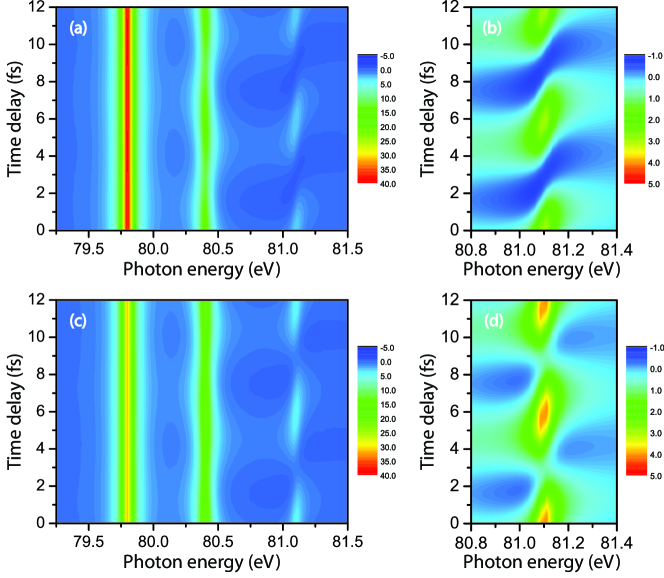
Figure 2: (Color online) Attosecond transient absorption cross section, in Mb, of strong-field-generated Kr⁺, plotted as a function of the photon energy and the time delay. The cross section was calculated using Eq. (35). Panels (a) and (b) show the attosecond transient absorption cross section for the theoretical ion density matrix elements in Table 1. In panels (c) and (d), the attosecond transient absorption cross section is shown for the experimental ion density matrix elements in Table 1.

The attosecond transient absorption cross sections [Eq. (35)] for the two sets of density matrix elements are plotted in Fig. 2. Again, there is no overlap between the NIR and EUV pulses, that is, the NIR pulse is centered at a large negative value of $t_{\mathrm{EUV}}$. The strongest of the three absorption lines does not depend on the time delay. This absorption line corresponds to a transition to the $3d_{5/2}^{-1}$ level. Since this level can be reached only from the $4p_{3/2}^{-1}$ level, but not from the $4p_{1/2}^{-1}$ level (see Fig. 1), the strongest absorption line is insensitive to the coherence between $4p_{3/2}^{-1}$ and $4p_{1/2}^{-1}$. The other two transitions, which both involve the $3d_{3/2}^{-1}$ level (see Fig. 1), display a conspicuous dynamical behavior as a function of the time delay. The modulation of the weakest line, which corresponds to the transition $4p_{3/2}^{-1}\rightarrow 3d_{3/2}^{-1}$, is most pronounced due to the coupling to the relatively strong $4p_{1/2}^{-1}\rightarrow 3d_{3/2}^{-1}$ transition. Moreover, for certain delays the absorption cross section for that line even becomes negative. This happens when the coherent population transfer from $4p_{1/2}^{-1}$ to $4p_{3/2}^{-1}$ via $3d_{3/2}^{-1}$ dominates over the absorption from the $4p_{3/2}^{-1}$ state.

Apart from the oscillation of the respective line strengths with the spin-orbit period of 6 fs, the energetic positions of the resonance lines oscillate as well. This is particularly easy to see in panels (b) and (d) in Fig. 2. These energy oscillations are a consequence of the interplay between the absorptive and dispersive terms mentioned earlier in connection with Eq. (35).

IV The accuracy of Beer’s law

In the previous section, our discussion was based on the approximation that different frequency components of the EUV pulse propagate independently. The assumption $\tilde{P}^{(1)}(x,\omega)\propto\tilde{\mathcal{E}}_{\mathrm{EUV}}(x,\omega)$ allowed us to describe the polarization response with a linear susceptibility $\chi^{(1)}(\omega)$ and to integrate Eq. (20) analytically. In this section, we investigate the accuracy of this approximation.

As follows from Eq. (30), the polarization response $\tilde{P}^{(1)}(x,\omega)$ is not proportional to $\tilde{\mathcal{E}}_{\mathrm{EUV}}(x,\omega)$ if the density matrix contains non-zero off-diagonal elements that correspond to states coupled by dipole transitions through an intermediate excited state. Physically, this means that an ion that absorbs a photon with an energy $\omega_{1}$ can coherently emit a photon with a different energy $\omega_{2}$, provided that the initial ionic state is a coherent superposition of two or more states. In this typical $\Lambda$-scheme, the polarization response at the photon energy $\omega_{2}$ obviously depends not only on $\tilde{\mathcal{E}}_{\mathrm{EUV}}(x,\omega_{2})$, but also on $\tilde{\mathcal{E}}_{\mathrm{EUV}}(x,\omega_{1})$. In this case, Eq. (21) is an approximation.

To go beyond this approximation, we numerically solve the first-order propagation equation (20) using Eq. (30) to evaluate the polarization response of the medium at each propagation step. Even though $\tilde{P}^{(1)}(x,\omega)$ is no longer proportional to $\tilde{\mathcal{E}}_{\mathrm{EUV}}(x,\omega)$, we compare the results of numerical propagation with those obtained in the previous section in terms of the apparent one-photon cross section:

$$\sigma_{\mathrm{app}}(\omega)=\frac{1}{n_{\mathrm{AT}}L}\ln\frac{\left|\tilde{\mathcal{E}}_{\mathrm{EUV}}(0,\omega)\right|^{2}}{\left|\tilde{\mathcal{E}}_{\mathrm{EUV}}(L,\omega)\right|^{2}}.$$ (36)

In Fig. 3, we show a false-color representation of $\sigma_{\mathrm{app}}(\omega)$ evaluated for different delays between the NIR pump and EUV probe pulses.

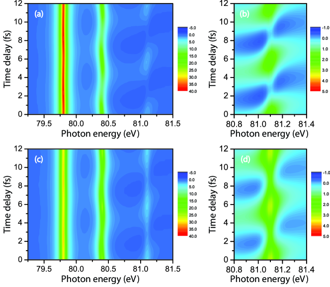
Figure 3: (Color online) Apparent attosecond transient absorption cross section, in Mb, of strong-field-generated Kr⁺, plotted as a function of the photon energy and the time delay. The cross section was calculated by applying Beer’s law to the numerically propagated EUV field. Panels (a) and (b) show the apparent attosecond transient absorption cross section for the theoretical ion density matrix elements in Table 1. In panels (c) and (d), the apparent attosecond transient absorption cross section is shown for the experimental ion density matrix elements in Table 1.

For this simulation, we used a bandwidth-limited Gaussian EUV pulse with a central photon energy of 80.8 eV and a full width at half maximum of intensity equal to 150 attoseconds. The elements of the density matrix were taken from Table 1. The propagation in a gas of strong-field-generated $\mbox{Kr}^{+}$ ions with an atomic number density of $n_{\mathrm{AT}}=2.2\times 10^{18}\ \mbox{cm}^{-3}$ was terminated after $L=1$ mm. The spectrum of the EUV pulse before and after propagation, for the experimental ion density matrix elements in Table 1, is shown in Fig. 4.

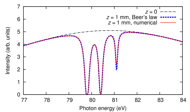
Figure 4: (Color online) The spectrum of the EUV pulse before (dash-dotted line) and after propagation for $t_{\mathrm{EUV}}=0$. The dashed line, representing a simulation assuming the validity of Beer’s law, corresponds to panels (c) and (d) in Fig. 2. The solid line shows the result of numerical propagation, corresponding to panels (c) and (d) in Fig. 3.

A careful inspection of Figs. 2, 3, and 4 reveals that the approximation underlying Beer’s law notably affects the line at 81.1 eV, which corresponds to the transition $4p_{3/2}^{-1}\rightarrow 3d_{3/2}^{-1}$. This is not surprising: for the same reasons why this absorption line exhibits strong quantum beats, it is also sensitive to other effects related to off-diagonal elements of the density matrix. Still, in spite of the strong absorption, the discrepancy between the model assuming the validity of Beer’s law and the results obtained by numerically solving the propagation equation is rather small.

It is instructive to repeat the analysis based on Eq. (35) and retrieve the density matrix from the apparent absorption cross section as if Beer’s law were rigorously valid. Table 2 gives these apparent density matrix elements. The good agreement between Tables 1 and 2 indicates that Beer’s law is indeed a good approximation for extracting electronic-structure information from transient absorption data, even though it should be used with care. We may conclude, in particular, that the discrepancy between the experimental and theoretical degrees of ion alignment ($j=3/2$ level) cannot be explained by a failure of Beer’s law.

Table 2: Apparent density matrix elements of strong-field-generated Kr⁺ ions extracted from the apparent attosecond transient absorption cross section for (a) the experimental ion density matrix elements in Table 1 and (b) the theoretical ion density matrix elements in Table 1.

	(a)	(b)
$2\rho^{(3/2)}_{3/2,3/2}$	0.21	0.03
$2\rho^{(1/2)}_{3/2,3/2}$	0.44	0.71
$2\rho^{(1/2)}_{1/2,1/2}$	0.35	0.26
$|\rho^{(1/2)}_{3/2,1/2}|$	0.14	0.14

V Conclusions

In this paper, we discussed the theory underlying attosecond transient absorption spectroscopy of strong-field-generated ions. This theory was employed in Ref. Goulielmakis_Nature_2010 to experimentally determine the reduced density matrix of Kr⁺ ions produced by an intense NIR pulse. Good agreement between experiment and theory was found for the degree of coherence and for the population of the $j=1/2$ level relative to the population of the $j=3/2$ level. However, experiment suggests strongly suppressed alignment of the $j=3/2$ level, which is not consistent with calculations based on the theory described in Ref. RoSa09 . The origin of this discrepancy is currently unknown.

As demonstrated in this paper, EUV propagation effects beyond Beer’s law do not explain the discrepancy between experiment and theory found for few-cycle NIR pulses Goulielmakis_Nature_2010 . Earlier measurements on Kr⁺ ions generated using 50 fs NIR pulses gave a degree of alignment in rather good agreement with an adiabatic strong-field-ionization theory SoAr07 . A noticeable reduction of ion alignment, in comparison to the adiabatic strong-field-ionization theory, was observed in Xe⁺ ions generated using 45 fs NIR pulses LoKh07 . But the effect was not as pronounced as it is in the current case, and it was surmised at the time that the discrepancy is a consequence of nonadiabatic effects LoKh07 . However, nonadiabatic effects cannot explain the disagreement between the experimental and theoretical ion density matrix elements shown in Table 1, for the strong-field-ionization theory employed RoSa09 is based on numerical wave-packet propagation and does not suffer from the limitations of the adiabatic approximation.

It seems likely that the origin of the discrepancy must be sought in either of the following two possibilities. The first possibility is that in the experiment of Ref. Goulielmakis_Nature_2010 , multielectron effects beyond the multichannel theory of Ref. RoSa09 played an important role. Since, in view of Ref. SoAr07 , these multielectron effects would appear to have a smaller impact when using longer NIR pulses, the observed discrepancy might suggest an enhancement of multielectron effects by few-cycle pulses. The second possibility is that the experiment of Ref. Goulielmakis_Nature_2010 was affected by substantial NIR propagation effects. This could be clarified by repeating the experiment at a lower target density.

- (1) M. Drescher, M. Hentschel, R. Kienberger, M. Uiberacker, V. Yakovlev, A. Scrinzi, T. Westerwalbesloh, U. Kleineberg, U. Heinzmann, and F. Krausz, Nature 419, 803 (2002).
- (2) F. Krausz and M. Ivanov, Rev. Mod. Phys. 81, 163 (2009).
- (3) J. Itatani, F. Quéré, G. L. Yudin, M. Yu. Ivanov, F. Krausz, and P. B. Corkum, Phys. Rev. Lett. 88, 173903 (2002)
- (4) R. Kienberger, E. Goulielmakis, M. Uiberacker, A. Baltuska, V. Yakovlev, F. Bammer, A. Scrinzi, T. Westerwalbesloh, U. Kleineberg, U. Heinzmann, M. Drescher, and F. Krausz, Nature 427, 817 (2004).
- (5) P. Eckle, M. Smolarski, P. Schlup, J. Biegert, A. Staudte, M. Schoeffler, H. G. Muller, R. Doerner, and U. Keller, Nature Physics 4, 565 (2008).
- (6) M. Schultze, M. Fieß, N. Karpowicz, J. Gagnon, M. Korbman, M. Hofstetter, S. Neppl, A. Cavalieri, Y. Komninos, Th. Mercouris, C. A. Nicolaides, R. Pazourek, S. Nagele, J. Feist, J. Burgdörfer, A. M. Azzeer, R. Ernstorfer, R. Kienberger, U. Kleineberg, E. Goulielmakis, F. Krausz, and V. S. Yakovlev, Science 328, 1658 (2010).
- (7) M. Uiberacker, Th. Uphues, M. Schultze, A. J. Verhoef, V. Yakovlev, M. F. Kling, J. Rauschenberger, and N. M. Kabachnik, H. Schroeder, M. Lezius, K. L. Kompa, H. G. Muller, M. J. J. Vrakking, S. Hendel, U. Kleineberg, U. Heinzmann, M. Drescher, and F. Krausz, Nature 446, 627 (2007).
- (8) E. Goulielmakis, Z.-H. Loh, A. Wirth, R. Santra, N. Rohringer, V. S. Yakovlev, S. Zherebtsov, T. Pfeifer, A. M. Azzeer, M. F. Kling, S. R. Leone, and F. Krausz, Nature 466, 739 (2010).
- (9) M. Dantus, M. J. Rosker, and A. H. Zewail, J. Chem. Phys. 87, 2395 (1987).
- (10) M. J. Rosker, M. Dantus, and A. H. Zewail, J. Chem. Phys. 89, 6113 (1988)
- (11) N. F. Scherer, D. M. Jonas, and G. R. Fleming, J. Chem. Phys. 99, 153 (1993).
- (12) D. M. Jonas, S. E. Bradforth, S. A. Passino, and G. R. Fleming, J. Phys. Chem. 99, 2594 (1995).
- (13) M. Saes, C. Bressler, R. Abela, D. Grolimund, S. L. Johnson, P. A. Heimann, and M. Chergui, Phys. Rev. Lett. 90, 047403 (2003).
- (14) C. Bressler and M. Chergui, Chem. Rev. 104, 1781 (2004).
- (15) L. Young, D. A. Arms, E. M. Dufresne, R. W. Dunford, D. L. Ederer, C. Höhr, E. P. Kanter, B. Krässig, E. C. Landahl, E. R. Peterson, J. Rudati, R. Santra, and S. H. Southworth, Phys. Rev. Lett. 97, 083601 (2006).
- (16) S. H. Southworth, D. A. Arms, E. M. Dufresne, R. W. Dunford, D. L. Ederer, C. Höhr, E. P. Kanter, B. Krässig, E. C. Landahl, E. R. Peterson, J. Rudati, R. Santra, D. A. Walko, and L. Young, Phys. Rev. A 76, 043421 (2007).
- (17) E. R. Peterson, C. Buth, D. A. Arms, R. W. Dunford, E. P. Kanter, B. Krässig, E. C. Landahl, S. T. Pratt, R. Santra, S. H. Southworth, and L. Young, Appl. Phys. Lett. 92, 094106 (2008).
- (18) L. X. Chen, W. J. H. Jäger, G. Jennings, D. J. Gosztola, A. Munkholm, and J. P. Hessler, Science 292, 262 (2001).
- (19) L. X. Chen, Ann. Rev. Phys. Chem. 56, 221 (2005).
- (20) W. T. Pollard and R. A. Mathies, Ann. Rev. Phys. Chem. 43, 497 (1992).
- (21) R. A. Mathies, C. H. Brito Cruz, W. T. Pollard, and C. V. Shank, Science 240, 777 (1988).
- (22) W. T. Pollard, S.-Y. Lee, and R. A. Mathies, J. Chem. Phys. 92, 4012 (1990).
- (23) Q. Wang, R. W. Schoenlein, L. A. Peteanu, R. A. Mathies, and C. V. Shank, Science 266, 422 (1994).
- (24) T. Kobayashi, T. Saito, and H. Ohtani, Nature 414, 531 (2001).
- (25) W. Graupner, G. Cerullo, G. Lanzani, M. Nisoli, E. J. W. List, G. Leising, and S. De Silvestri, Phys. Rev. Lett. 81, 3259 (1998).
- (26) V. I. Klimov, J. Phys. Chem. B 104, 6112 (2000).
- (27) U. Megerle, I. Pugliesi, C. Schriever, C. F. Sailer and E. Riedle, Appl. Phys. B 96, 215 (2009).
- (28) F. Raksi, K. R. Wilson, Z. Jiang, A. Ikhlef, C. Y. Cote, and J.-C. Kieffer, J. Chem. Phys. 104, 6066 (1996).
- (29) Z.-H. Loh, M. Khalil, R. E. Correa, R. Santra, C. Buth, and S. R. Leone, Phys. Rev. Lett. 98, 143601 (2007).
- (30) E. Seres and C. Spielmann, Appl. Phys. Lett. 91, 121919 (2007).
- (31) Z.-H. Loh and S. R. Leone, J. Chem. Phys. 128, 204302 (2008).
- (32) Z.-H. Loh, C. H. Greene, and S. R. Leone, Chem. Phys. 350, 7 (2008).
- (33) A. Cavalleri, M. Rini, H. H. W. Chong, S. Fourmaux, T. E. Glover, P. A. Heimann, J. C. Kieffer, and R. W. Schoenlein, Phys. Rev. Lett. 95, 067405 (2005).
- (34) C. Höhr, E. R. Peterson, N. Rohringer, J. Rudati, D. A. Arms, E. M. Dufresne, R. W. Dunford, D. L. Ederer, E. P. Kanter, B. Krässig, E. C. Landahl, R. Santra, S. H. Southworth, and L. Young, Phys. Rev. A 75, 011403(R) (2007).
- (35) R. Santra, R. W. Dunford, and L. Young, Phys. Rev. A 74, 043403 (2006).
- (36) N. Rohringer and R. Santra, Phys. Rev. A 79, 053402 (2009).
- (37) A. L. Fetter and J. D. Walecka, Quantum Theory of Many-Particle Systems (McGraw-Hill, Boston, 1971).
- (38) R. D. Mattuck, A Guide to Feynman Diagrams in the Many-Body Problem (Dover, New York, 1992).
- (39) N. H. March, W. H. Young, and S. Sampanthar, The Many-Body Problem in Quantum Mechanics (Dover, New York, 1995).
- (40) F. A. Parpia, C. Froese-Fischer, and I. P. Grant, Comput. Phys. Commun. 94, 249 (1996).
- (41) A. R. Edmonds, Angular Momentum in Quantum Mechanics (Princeton University Press, Princeton, 1957).
- (42) U. Fano and G. Racah, Irreducible Tensorial Sets (Academic Press, New York, 1959).
- (43) R. N. Zare, Angular Momentum: Understanding Spatial Aspects in Chemistry and Physics (Wiley, New York, 1988).
- (44) M. Jurvansuu, A. Kivimäki, and S. Aksela, Phys. Rev. A 64, 012502 (2001).