An Einstein-Bianchi system for
Smooth Lattice General Relativity. I.
The Schwarzschild spacetime.

Abstract

The second Bianchi identity can be recast as an evolution equation for the Riemann curvatures. Here we will report on such a system for a vacuum static spherically symmetric spacetime. This is the first of two papers. In the following paper we will extend the ideas developed here to general vacuum spacetimes. In this paper we will demonstrate our ideas on a Schwarzschild spacetime and give detailed numerical results. For suitable choices of lapse function we find that the system gives excellent results with long term stability.

1 Introduction

Despite a slow start, hyperbolic formulations of the Einstein equations have in recent times become the system of choice for numerical relativity.

The confidence afforded to hyperbolic systems is borne out not just by the recent success in numerical relativity [1, 2, 3] but also from their strict mathematical underpinnings (which guarantees that future evolutions exist and that they depend smoothly on the initial data, these are key aspects of the theorems that demonstrate the stability of the system, see [4] for details).

One of the earlier hyperbolic formulations was given by Friedrich [5] in which he used the second Bianchi identities to evolve the Weyl curvatures in-situ with the metric. This idea has been extended by many other authors [6, 7, 8, 9] and the resulting equations are commonly referred to as an Einstein-Bianchi system.

Yet despite their mathematical elegance and the virtues that this would bestow upon a numerical code there seems to be have been very few numerical applications employing an Einstein-Bianchi system (though see [10, 11]).

In this paper we will report on a simple Einstein-Bianchi system adapted to a discrete lattice for static spherically symmetric spacetimes. We were lead to this formulation not by way of Friedrich’s paper but rather as a direct extension of our own ideas developed in an earlier series of papers [12, 13, 14, 15]. In those papers we used the spatial form of the second Bianchi identities (i.e., the second Bianchi identity for the 3-metric) to compute the 3-Riemann curvatures across a Cauchy surface. This device proved to be the key element in obtaining accurate and stable evolutions of the initial data.

Our longer term intention is to employ an Einstein-Bianchi system to evolve a 3-dimensional lattice. This will require not only evolution equations for the legs of the lattice, such as those given in [13], but also evolution equations for the curvatures. This will be the subject of the second paper in this series.

For the simple case presented here we find that the system works very well. The evolutions are stable, though this depends on the choice of the lapse function, see sections (4.1) and (6.1). We also find that the constraints are well behaved (they appear to grow linearly with time and converge to zero as the lattice is refined, see section (6.2)).

As this paper borrows heavily from two of our previous papers, which we refer to as Paper 1 and Paper 2, we will skip over many of the derivations and arguments assuming instead that the reader is familiar with the material in Paper 1 and Paper 2.

2 Spherically symmetric spacetimes

In this paper we will be constructing lattice approximations to the Schwarzschild spacetime in various slicings. In each case the continuum metric can be written in the form

$$ds^{2}=-N(r,t)^{2}dt^{2}+A(r,t)^{2}dr^{2}+B(r,t)^{2}d\Omega^{2}$$ (2.1)

for some set of functions $N(r,t)$, $A(r,t)$, $B(r,t)$ and where $d\Omega^{2}=d\theta^{2}+\sin^{2}\theta d\phi^{2}$ is the metric of the unit 2-sphere. We have introduced this coordinate form of the continuum metric simply as a precursor to the introduction of the lattice. As we shall soon see, we will use the coordinate lines and their local tangent vectors as a scaffold on which to build the lattice, after which we will have no further need for the coordinates (indeed we could dispense with the coordinates altogether at the possible expense of the clarity of the exposition).

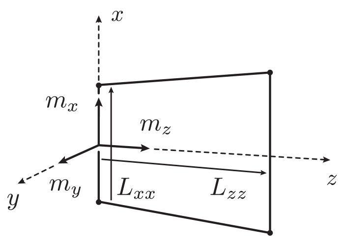
Figure 2: The local structure of the lattice. The $(x,y,z)$ are a set of coordinates local to this set of legs. There is one such coordinate frame for each $L_{xx}$ along the lattice. These coordinates are never used in the computer code but help to define the metric in the neighbourhood of $L_{xx}$.

Consider a local orthonormal tetrad built from the future pointing unit normal $t^{\mu}$ to a typical Cauchy surface and three unit vectors $m^{\mu}_{x}$, $m^{\mu}_{y}$ and $m^{\mu}_{z}$ where $m^{\mu}_{z}$ is parallel to the radial axis (see figure (2)). These basis vectors are also tangent vectors to the coordinate axes of a local Riemann normal frame. We will use this tetrad to record the frame components of the extrinsic and Riemann curvatures on the lattice. Our notation, which we borrow from Paper 1, will be to use script characters to denote frame quantities, thus ${{\cal K}}_{xx}:=K_{\mu\nu}m^{\mu}_{x}m^{\nu}_{x}$ while ${\cal R}_{tztz}:=R_{\mu\alpha\nu\beta}t^{\mu}m^{\alpha}_{z}t^{\nu}m^{\beta}_{z}$. Also, to avoid an overflow of symbols, we will allow $L_{xx}$ and $L_{zz}$ to represent both the length of the corresponding leg as well the leg itself.

In this class of spacetimes, and on this tetrad, we know that the extrinsic curvature is diagonal and that a basis for the non-trivial Riemann curvatures is given by

$${\cal R}_{xyxy},\quad{\cal R}_{xzxz},\quad{\cal R}_{txtx},\quad{\cal R}_{tztz},\quad{\cal R}_{txxz}$$

Now using $R_{\mu\nu}=R^{\alpha}{}_{\mu\alpha\nu}$ and $R=g^{\mu\nu}R_{\mu\nu}$ we find

$${\cal R}_{tz} =-2{\cal R}_{txxz}$$ (2.2)

$${\cal R}_{tt} ={\cal R}_{tztz}+2{\cal R}_{txtx}$$ (2.3)

$${\cal R}_{zz} =-{\cal R}_{tztz}+2{\cal R}_{xzxz}$$ (2.4)

$${\cal R}_{xx} =-{\cal R}_{txtx}+{\cal R}_{xyxy}+{\cal R}_{xzxz}$$ (2.5)

$${\cal R} =-4{\cal R}_{txtx}-2{\cal R}_{tztz}+2\left({\cal R}_{xyxy}+2{\cal R}_{xzxz}\right)$$ (2.6)

while the non-trivial vacuum Einstein equations yield

$${\cal R}_{tz}={\cal R}_{tt}={\cal R}_{zz}={\cal R}_{xx}=0$$ (2.7)

Combining the above shows that we can express all of the non-trivial Riemann curvatures solely in terms of ${\cal R}_{xyxy}$ and ${\cal R}_{xzxz}$, namely

$${\cal R}_{txxz} =0$$ (2.8)

$${\cal R}_{tztz} =2{\cal R}_{xzxz}$$ (2.9)

$${\cal R}_{txtx} ={\cal R}_{xyxy}+{\cal R}_{xzxz}$$ (2.10)

In obtaining these relations we used $g^{\mu\nu}=-t^{\mu}t^{\nu}+m^{\mu}_{x}m^{\nu}_{x}+m^{\mu}_{y}m^{\nu}_{y}+m^{\mu}_{z}m^{\nu}_{z}$.

Note that ${\cal R}_{xyxy}$ and ${\cal R}_{xzxz}$ are not independent for the simple equation $R=0$ leads to

$$0={\cal R}_{xyxy}+2{\cal R}_{xzxz}$$ (2.11)

We will use this equation as a check on our numerical integrations (see section (6.2) for more details).

3 The lattice

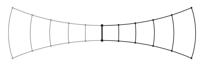
Figure 1: A simple lattice for a Schwarzschild spacetime. This consists of two identical halves joined at the throat (denoted by the thick line). In our computer code we only store the right hand half (plus a few nodes from the left half to ensure reflection symmetry at the throat).

The symmetries in the Schwarzschild spacetime allows us to use a very simple ladder-like structure for the lattice, as indicated in figure (1). One way to imagine the construction of the lattice is to consider the coordinate mesh generated by setting $t={}$constant and $\theta=\pi/2$ in the coordinate form of the metric in (2.1). Then the rungs of the ladder are generated by small increments in $\phi$ leading to $L_{xx}\approx B\Delta\phi$ while the side rails would coincide with two radial curves (i.e., $\phi={}$constant) with $L_{zz}\approx A\Delta r$. Clearly, specifying all of the $L_{xx}$ and $L_{zz}$ is equivalent to specifying the metric components $A(r,t)$ and $B(r,t)$. Note that throughout this paper we treat the $L_{xx}$ and $L_{zz}$ as continuous functions of time.

We will label the nodes from $0$ to $n$ and on the few occasions where we need to discuss more than one leg at a time we will write $(L_{xx})_{i}$ to denote an $L_{xx}$ leg at node $i$. In the same way $(L_{zz})_{i}$ will denote the $L_{zz}$ that joins the nodes $i$ and $i+1$. Similar notation will be used for other data on the lattice.

The initial data (as described in section (5)) are constructed in a way that guarantees reflection symmetry at the throat (which is always tied to node 0).

In our computer code we extend our lattice a small way over the throat, by including the nodes -3 to -1, so that we can readily impose the reflection symmetries (by simply copying data across the throat, at no point do we independently evolve any of the data to the left of the throat).

4 The evolution equations

Our present task is to develop evolution equations for the leg-lengths, the extrinsic curvatures and, the principle innovation in this paper, evolution equations for the Riemann curvatures.

A simple derivation of the evolution equations for our lattice can be obtained from a general pair of equations developed in Paper 2. There it was shown that the first and second variations of arc lengths can be written in a form remarkably similar to the ADM equations, namely

$$\frac{dL_{ij}^{2}}{dt} =-2NK_{\mu\nu}\Delta x^{\mu}_{ij}\Delta x^{\nu}_{ij}+\mathcal{O}\left(L^{3}\right)$$ (4.1)

$$\frac{d\ }{dt}\left(\frac{1}{N}\frac{dL_{ij}^{2}}{dt}\right) =2N_{|\alpha\beta}\Delta x_{ij}^{\alpha}\Delta x_{ij}^{\beta}$$ (4.2)

$$\quad+2N\left(K_{\mu\alpha}K^{\mu}{}_{\beta}-R_{\mu\alpha\nu\beta}t^{\mu}t^{\nu}\right)\Delta x_{ij}^{\alpha}\Delta x_{ij}^{\beta}+\mathcal{O}\left(L^{3}\right)$$

Note that in the following we will ignore the leading error terms $\mathcal{O}\left(L^{3}\right)$. Applying these equations to the two legs $L_{xx}$ and $L_{zz}$ of our spherically symmetric lattice leads immediately to

$$\frac{dL_{xx}}{dt} =-N{{\cal K}}_{xx}L_{xx}$$ (4.3)

$$\frac{dL_{zz}}{dt} =-N{{\cal K}}_{zz}L_{zz}$$ (4.4)

$$\frac{d{{\cal K}}_{xx}}{dt} =-{N_{,xx}}+N\left({\cal R}_{txtx}+{{\cal K}}_{xx}^{2}\right)$$ (4.5)

$$\frac{d{{\cal K}}_{zz}}{dt} =-{N_{,zz}}+N\left({\cal R}_{tztz}+{{\cal K}}_{zz}^{2}\right)$$ (4.6)

The last part of the picture is to provide evolution equations for the Riemann curvatures, ${\cal R}_{xyxy}$ and ${\cal R}_{xzxz}$. The basic idea is to rearrange the terms in the Bianchi identities to isolate the time derivatives while estimating the spatial derivatives from data imported from neighbouring cells. The calculations are straight-forward but a bit tedious to present here so we defer the full details to the Appendix. This leads to the following evolution equations

$$\frac{d{\cal R}_{xyxy}}{dt} =2N{{\cal K}}_{xx}\left(2{\cal R}_{xyxy}+{\cal R}_{xzxz}\right)$$ (4.7)

$$\frac{d{\cal R}_{xzxz}}{dt} =3N{{\cal K}}_{xx}{\cal R}_{xzxz}+N{{\cal K}}_{zz}\left({\cal R}_{xyxy}+2{\cal R}_{xzxz}\right)$$ (4.8)

The Riemann curvatures ${\cal R}_{xyxy}$ and ${\cal R}_{xzxz}$ would normally not be evolved but rather derived from the lattice data such as the leg lengths $L_{xx}$ and $L_{zz}$. In Paper 1 we used (discrete versions of) the geodesic deviation equation and the spatial Bianchi identity

$$0 =\frac{d^{2}L_{xx}}{dz^{2}}+{}^{3}{\cal R}_{xzxz}L_{xx}$$ (4.9)

$$0 =\frac{d\left(L^{2}_{xx}{}^{3}{\cal R}_{xyxy}\right)}{dz}-{}^{3}{\cal R}_{xzxz}\frac{dL^{2}_{xx}}{dz}$$ (4.10)

to compute the 3-dimensional Riemann curvatures ${}^{3}{\cal R}_{xyxy}$ and ${}^{3}{\cal R}_{xzxz}$ on the lattice. In raising the ${\cal R}_{xyxy}$ and ${\cal R}_{xzxz}$ to dynamical variables on the lattice we are forced to view equations (4.9,4.10) as constraints on the lattice data. In section (6.2) we shall present discretised versions of these constraints which we will later use to check the quality of our numerical results.

The one remaining constraint is the standard momentum constraint (see Paper 1 for details)

$$0=\frac{d(L_{xx}{{\cal K}}_{xx})}{dz}-{{\cal K}}_{zz}{\frac{dL_{xx}}{dz}}$$ (4.11)

4.1 Artificial viscosity

Our numerical experiments (which we will present shortly) showed that the future evolutions can be subject to high-frequency instabilities. This was seen to occur only in the cases where the lapse function was controlled by its own evolution equation (e.g., as in Harmonic slicing). For such cases we found that stability could be recovered with the addition of an artificial viscosity term to the evolution equations.

Let $W$ be any one of the dynamical variables, $L_{xx}$, $L_{zz}$, ${{\cal K}}_{xx}$, ${{\cal K}}_{zz}$. Then the artificial viscosity is introduced by the addition of a simple dissipation term to the evolution equation for $W$. After some experimentation we settled on the following form

$$\frac{dW_{i}}{dt}=\frac{d{\bar{W}}_{i}}{dt}+\mu N_{i}\left(\frac{W_{i+1}-W_{i}}{(L_{zz})_{i}}-\frac{W_{i}-W_{i-1}}{(L_{zz})_{i-1}}\right)$$ (4.12)

where $d{\bar{W}}_{i}/dt$ is the right hand side of the original evolution equation (4.3–4.6) and $\mu$ is a (small) constant. Other choices were tried but this form seemed to produce stable evolutions for the longest periods of time. Note that we do not add the dissipation terms to the evolution equations for the curvatures (doing so seemed to make no difference to the evolutions and had no effect in controlling the instabilities).

How should $\mu$ be chosen? We need to choose it large enough to ensure that the evolution is stable over a given time interval while also keeping it sufficiently small so as to not effect the large scale features of the numerical solution. By trial and error we found that setting $\mu=0.08$ worked well for evolutions to $t=100.0$ using $n=2048$ nodes. We also found that as the number of nodes was increased we had to make a proportionate increase in $\mu$ to maintain the same quality of the evolution over the same time interval. That is $\mu=\mathcal{O}\left(n\right)$.

The dissipation term is easily seen to be a finite difference approximation to $\mu L_{zz}d^{2}W/dz^{2}$ and thus it may appear to be like a Kreiss-Oliger term that vanishes in the continuum limit. However, since we are forced to set $\mu=\mathcal{O}\left(n\right)$ and as $L_{zz}=\mathcal{O}\left(1/n\right)$ we see that the term $\mu L_{zz}$ is approximately constant, say $\mu^{\prime}$, and thus the dissipation term is actually of the form $\mu^{\prime}d^{2}W/dz^{2}$. This is a standard dissipation term commonly used in hydrodynamic simulations and it does not vanish in the continuum limit.

5 Initial data

The initial data on the lattice are the $L_{xx}$, $L_{zz}$, ${{\cal K}}_{xx}$, ${{\cal K}}_{zz}$, ${\cal R}_{xyxy}$ and ${\cal R}_{xzxz}$ at each node of the lattice. Their time symmetric initial values were set by a combination of the Hamiltonian constraint, the geodesic deviation equation and the Bianchi identities. A full account of the choices made in coming to the equations described below can be found Paper 1. Here we will just quote the relevant equations simply to provide explicit details of how we constructed our initial data.

To ensure that the initial data is time symmetric we set ${{\cal K}}_{xx}=0$ and ${{\cal K}}_{zz}=0$.

The $L_{zz}$ were set according to the method of Bernstein, Hobill and Smarr [16] using $n=2048$ on a grid of length $800.0{}m$. The ADM mass, $m$, was set to be $1.0$ and the $L_{xx}$, ${\cal R}_{xyxy}$ and ${\cal R}_{xzxz}$, for $i=1,2,3\dots n$, were set according to

$$(L_{xx})_{i} =(L_{xx})_{i-1}+\frac{(L_{zz})_{i-1}}{(L_{zz})_{i-2}}\left((L_{xx})_{i-1}-(L_{xx})_{i-2}\right)$$

$$\quad-\frac{1}{2}(L_{zz})_{i-1}\left((L_{zz})_{i-1}+(L_{zz})_{i-2}\right)\left(L_{xx}{\cal R}_{xzxz}\right)_{i-1}$$ (5.1)

$$({\cal R}_{xzxz})_{i} =({\cal R}_{xzxz})_{i-1}\left(\frac{5\left(L^{2}_{xx}\right)_{i-1}-\left(L^{2}_{xx}\right)_{i}}{5\left(L^{2}_{xx}\right)_{i}-\left(L^{2}_{xx}\right)_{i-1}}\right)$$ (5.2)

$$({\cal R}_{xyxy})_{i} =-2({\cal R}_{xzxz})_{i}$$ (5.3)

At the reflection symmetric throat (i.e., at node 0) we set $(L_{xx})_{0}=0.01$ and $({\cal R}_{xyxy})_{0}=-2({\cal R}_{xzxz})_{0}=0.25$.

6 Results

In all of our results we used a 4-th order Runge-Kutta integrator with the time step set equal to $1/2$ the smallest $L_{zz}$ on the lattice (which happens to be $(L_{zz})_{0}$).

6.1 Slicing conditions

We ran our code for eight distinct slicing conditions, some were set by simple algebraic expressions while others involved differential operators.

We made four choices for the algebraic slicings,

$$N =\exp(-2{{\cal K}}_{xx})$$ (6.1)

$$N =\frac{20L_{xx}}{1+20L_{xx}}$$ (6.2)

$$N =\exp(-{\cal R}_{xyxy})$$ (6.3)

$$N =\frac{1}{1+{\cal R}_{xyxy}}$$ (6.4)

and three choice for the differential slicings,

$$1+\log \frac{dN}{dt}=-2NK$$ slicing (6.5)

Harmonic slicing $$\frac{dN}{dt}=-N^{2}K$$ (6.6)

Maximal slicing $$\nabla^{2}N={}^{3}RN$$ (6.7)

The eighth slicing condition was the simple case of geodesic slicing $N=1$.

The algebraic slicings were introduced after our early explorations with the differential lapses, all of which developed high-frequency instabilities after a short time (well before $t=100$). The algebraic slicings did not require any artificial viscosity and performed remarkably well, showing no signs of instabilities to at least $t=1000$ (excluding the lapse (6.2) which hits the singularity at $t\approx 32$). We have not run our codes beyond $t=1000$ so we can not comment its stability for $t>1000$.

6.2 Code tests and results

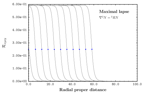
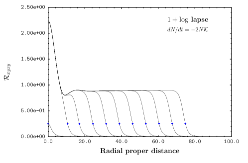
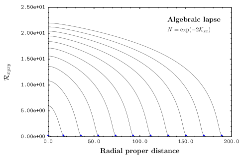
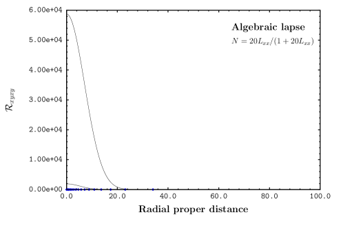
Figure 5: The curvature profiles for four choices of lapse function. Each figure shows the lapse function for $t=0$ to $t=100$ in steps of 10. The small diamond on each curve represents the location of the apparent horizon. There are only two curves visible in the algebraic slicing $N=20L_{xx}/(1+20L_{xx})$ due to the rapid rise in the curvatures as the slicing approaches the singularity.

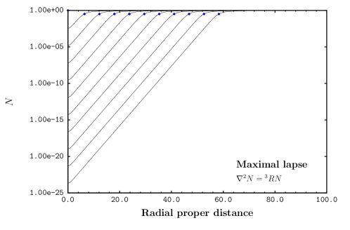
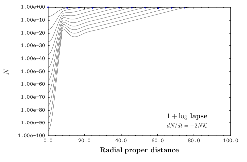
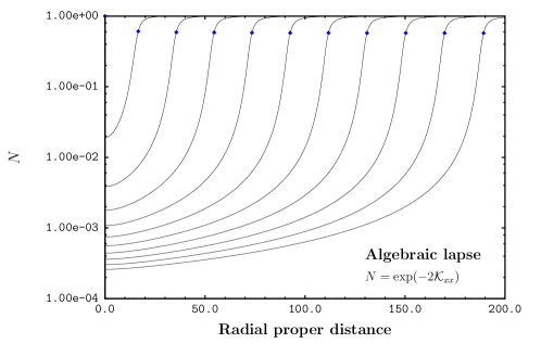
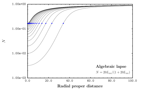
Figure 6: As per figure (5) but this time we display the lapse profiles. Note how quickly the lapse collapse at the throat in the $1+\log{}$ slicing. This would likely cause serious underflow problems for $t\gtrsim 300$. Notice also the uniform spacing of the curves along the logarithmic axis for the maximal lapse. This show that the lapse collapses exponentially at the throat (a well known result for maximal slicing).

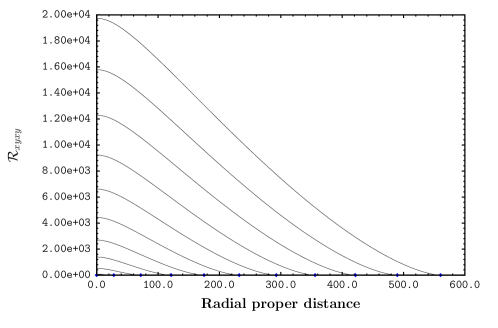
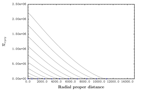
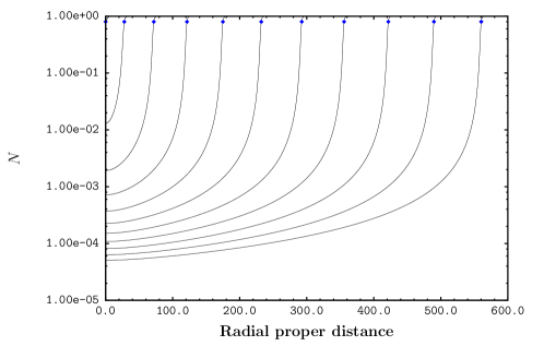
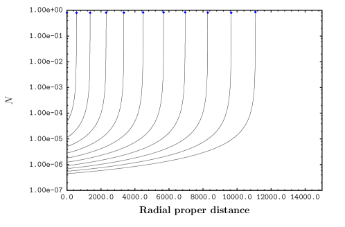
Figure 7: The Riemann curvature ${\cal R}_{xyxy}$ and the lapse function $N$ for the algebraic slicing with $N=1/(1+{\cal R}_{xyxy})$. The left pair of figures shows the evolution over the range $t=0$ to 100 in steps of 10, while the right pair cover the range $t=0$ to $1000$ in steps of 100. This lapse does not appear (on this time scale) to exhibit an exponential collapse at the throat. The profiles for the algebraic slicings appear to propagate into the asymptotically flat regions far more rapidly than any of the differential slicings. This may be explain why an artificial viscosity was not needed for the algebraic slicings – they carry away any small numerical errors before they have chance to grow.

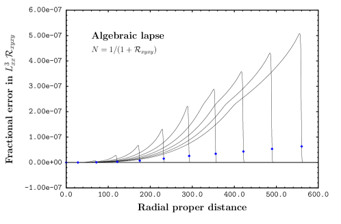
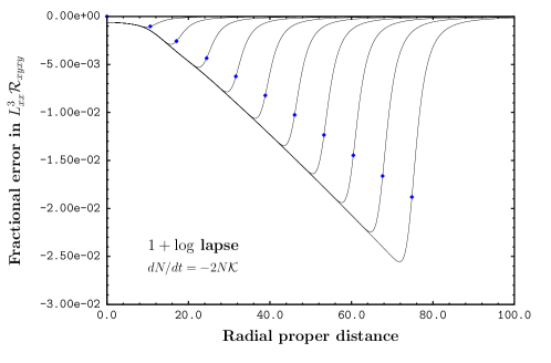
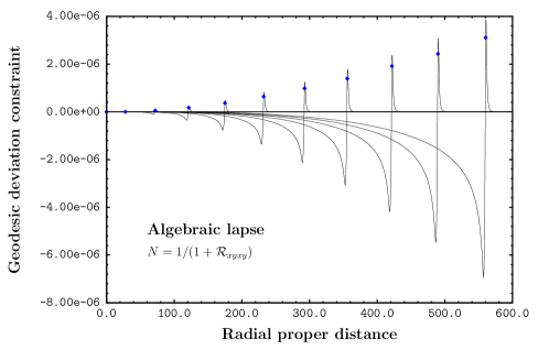
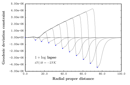
Figure 9: According to equation (6.9) the quantity $L_{xx}^{3}{\cal R}_{xyxy}$ should be conserved. In the top row we display the relative error, defined by $1-C(t)/C(0)$ with $C(t)=L_{xx}^{3}(t){\cal R}_{xyxy}(t)$, for two choices of lapse. The errors for the $1+\log$ slicing are much larger than those for the algebraic slicing which we attribute to the action of the artificial viscosity terms. In the bottom row we display the momentum constraint for the same pair of slicings. This shows a slow growth in the momentum constraint over time (judging by the peaks in the plots, the growth appears to be linear in time).

We subjected our code to many of the tests used in Paper 1, such as the time at which geodesic slicing hits the singularity, the rate at which the lapse at the throat collapses in maximal slicing and the constancy of $L_{xx}$ on the horizon. The results for these various slicings are shown in figures (4–9). All of the results are as expected. For the geodesic slicing the code crashes at approximately one time step short of the singularity. The familiar exponential collapse of the lapse for maximal slicing is evident in figure (6). In this case it is known that the lapse at the throat should behave as $N\sim\beta\exp(\alpha t)$ for $t\rightarrow\infty$ with $\alpha=-(2/3)^{(3/2)}\approx-0.54433$, see [17]. We estimated the slope of $\ln N$ vs $t$ from our numerical data to be $-0.54215$ which agrees with the exact value to within $0.4$ percent.

We also have a new test obtained by a simple combination of the evolution equations. From equations (4.7,4.8) we find that

$$\frac{d\left({\cal R}_{xyxy}+2{\cal R}_{xzxz}\right)}{dt}=2N\left(2{{\cal K}}_{xx}+{{\cal K}}_{zz}\right)\left({\cal R}_{xyxy}+2{\cal R}_{xzxz}\right)$$ (6.8)

and as $0={\cal R}_{xyxy}+2{\cal R}_{xzxz}$ on the initial slice (by construction, see (5.3)) we conclude that $0={\cal R}_{xyxy}+2{\cal R}_{xzxz}$ for all time. This is not surprising, our evolution equations for the curvatures are based on the Bianchi identities and these are guaranteed to preserve the constraints. If we now set $0={\cal R}_{xyxy}+2{\cal R}_{xzxz}$ in (4.8) and combine the result with (4.3) we find

$$0=\frac{dL_{xx}^{3}{\cal R}_{xyxy}}{dt}$$ (6.9)

This gives us a new test of our code, that the quantity $L_{xx}^{3}{\cal R}_{xyxy}$ should be constant throughout the evolution. Importantly this applies to all slicing conditions. In figure (9) we have plotted the fractional variations in $L_{xx}^{3}{\cal R}_{xyxy}$ for two choices of slicings. We see that the errors for the $1+\log$ slicing are much larger than those for the algebraic slicing which we attribute to the use of an artificial viscosity. This last claim is easily checked by varying the artificial viscosity parameter $\mu$. We find that the errors in $L_{xx}^{3}{\cal R}_{xyxy}$ varies linearly with $\mu$. Note that in obtaining equation (6.9) we have ignored the higher order error terms that would arise if we had carried through the $\mathcal{O}\left(L^{3}\right)$ truncation error from (4.1). Thus even if we set $\mu=0$ we can expect some variation of $L_{xx}^{3}{\cal R}_{xyxy}$ over time (though this variation should vanish more rapidly than $\mathcal{O}\left(L^{3}\right)$).

We also have three constraint equations, namely the geodesic deviation equation (4.9), the 3-dimensional Bianchi identity (4.10) and the momentum constraint (4.11). The discrete form of these equations are

$$P =\frac{D^{2}L_{xx}}{Dz^{2}}+{}^{3}{\cal R}_{xzxz}L_{xx}$$ (6.10)

$$Q =\frac{{\tilde{D}}\left(L^{2}_{xx}{}^{3}{\cal R}_{xyxy}\right)}{Dz}-{}^{3}{\tilde{\cal R}_{xzxz}}\frac{{\tilde{D}}L_{xx}^{2}}{Dz}$$ (6.11)

$$M =\frac{D\left(L_{xx}{{\cal K}}_{xx}\right)}{Dz}-{{\cal K}}_{zz}\frac{DL_{xx}}{Dz}$$ (6.12)

where ${\tilde{\cal R}_{xzxz}}$ is the average of ${\cal R}_{xzxz}$ across $L_{zz}$ while $D/Dz$ and ${\tilde{D}}/Dz$ are discrete derivative operators defined as follows. For a typical smooth function $f(z)$ sampled at the grid points $z_{i}$ we define

$$\left(\frac{{\tilde{D}}f}{Dz}\right)_{i} :=\frac{f^{\hbox{\small\tt+}}-f^{\hbox{\small\tt o}}}{L_{zz}^{\hbox{\small\tt o}}}$$ (6.13)

$$\left(\frac{Df}{Dz}\right)_{i} :=\frac{1}{L_{zz}^{\hbox{\small\tt o}}+L_{zz}^{\hbox{\small\tt-}}}\left(L_{zz}^{\hbox{\small\tt-}}\left(\frac{f^{\hbox{\small\tt+}}-f^{\hbox{\small\tt o}}}{L_{zz}^{\hbox{\small\tt o}}}\right)+L_{zz}^{\hbox{\small\tt o}}\left(\frac{f^{\hbox{\small\tt o}}-f^{\hbox{\small\tt-}}}{L_{zz}^{\hbox{\small\tt-}}}\right)\right)$$ (6.14)

$$\left(\frac{D^{2}f}{Dz^{2}}\right)_{i} :=\frac{2}{L_{zz}^{\hbox{\small\tt o}}+L_{zz}^{\hbox{\small\tt-}}}\left(\frac{f^{\hbox{\small\tt+}}-f^{\hbox{\small\tt o}}}{L_{zz}^{\hbox{\small\tt o}}}-\frac{f^{\hbox{\small\tt o}}-f^{\hbox{\small\tt-}}}{L_{zz}^{\hbox{\small\tt-}}}\right)$$ (6.15)

where we have introduced the superscripts +, o and - to denote quantities at the grid points $z_{i+1}$, $z_{i}$ and $z_{i-1}$ respectively. Note that the sample points $z_{i}$ are constructed from the lattice $L_{zz}$ by the recurrence relation $z_{i+1}=z_{i}+(L_{zz})_{i}$ with $z_{0}=0$. In this notation we have ${\tilde{\cal R}}_{xyxy}:=({\cal R}_{xyxy}^{{\hbox{\small\tt+}}}+{\cal R}_{xyxy}^{{\hbox{\small\tt o}}})/2$. Finally we note that the 3-curvatures can be computed from the 4-curvatures by way of the Gauss equation,

$${}^{3}{\cal R}_{xyxy} ={\cal R}_{xyxy}-{{\cal K}}_{xx}^{2}$$ (6.16)

$${}^{3}{\cal R}_{xzxz} ={\cal R}_{xzxz}-{{\cal K}}_{xx}{{\cal K}}_{zz}$$ (6.17)

Ideally we would like to see $P=Q=M=0$ but in reality we expect $P_{i}$, $Q_{i}$ and $M_{i}$ to be non-zero but small. This is indeed what we observe, see figure (9). We also computed a crude estimate of the rate of convergence (of $Q$, $P$ and $M$ to zero at a fixed time) by running our code twice, once with $n=2048$ and once with $n=1024$ and then forming suitable ratios of the constraints at the horizon. In this manner we estimated, in the absence of artificial viscosity, that $P=\mathcal{O}\left(n^{-4}\right)$, $Q=\mathcal{O}\left(n^{-2}\right)$ and $M=\mathcal{O}\left(n^{-3}\right)$ while the addition of artificial viscosity degraded the convergence to $P=\mathcal{O}\left(n^{-1}\right)$, $Q=\mathcal{O}\left(n^{-1}\right)$ and $M=\mathcal{O}\left(n^{-2}\right)$.

We also tried setting ${\tilde{D}}/Dz:=D/Dz$ and ${\tilde{\cal R}}_{xyxy}:={\cal R}_{xyxy}^{{\hbox{\small\tt o}}}$ in the discrete Bianchi constraint but this lead to a reduction in the rate of convergence. The form of the discrete Bianchi constraint as given above (6.11) is readily seen [14] to be a second-order accurate estimate to the continuum Bianchi identity at the centre of the leg $L_{zz}$.

One might ask why we have not included the Hamiltonian constraint in our code tests. The simple answer is that it is trivially satisfied by our discrete equations. This follows from the discussion surrounding equation (6.8) where we showed that $0={\cal R}_{xyxy}+2{\cal R}_{xzxz}$ for all time. It follows that the Hamiltonian $H:=G_{\mu\nu}t^{\mu}t^{\mu}$ will also vanish for all time. Note that this analysis was based on our discrete equations, not on the continuum equations. We did indeed check that our code maintained $0={\cal R}_{xyxy}+2{\cal R}_{xzxz}$ throughout the evolution.

Appendix A Bianchi identities

Here we will use the Bianchi identities to obtain evolution equations for the two curvatures ${\cal R}_{xyxy}$ and ${\cal R}_{xzxz}$. We will follow the method given in our earlier paper [14] in which we used data imported from the neighbouring computational cells to estimate (by a finite difference approximation) the various derivatives required in the Bianchi identities. We will employ Riemann normal coordinates, one for each computational cell, with the origin centred on the central vertex and the coordinate axes aligned with those described in section (2), see also figure (2). In these coordinates, the metric in a typical computational cell is given by

$$g_{\mu\nu}(x)=g_{\mu\nu}-\frac{1}{3}R_{\mu\alpha\nu\beta}x^{\alpha}x^{\beta}-\frac{1}{6}R_{\mu\alpha\nu\beta,\gamma}x^{\alpha}x^{\beta}x^{\gamma}+\mathcal{O}\left(L^{4}\right)\\$$

where $L$ is a typical length scale for the computational cell and $g_{\mu\nu}$ and $R_{\mu\alpha\nu\beta}$ are constant throughout the computational cell. A convenient choice for $g_{\mu\nu}$ is ${\rm diag}(-1,1,1,1)$ (such a choice can always be made by suitable gauge transformations within the class of Riemann normal frames). In this case the frame components ${\cal R}_{xyxy}$ and ${\cal R}_{xzxz}$ reduce to the coordinate components $R_{xyxy}$ and $R_{xzxz}$ respectively. A further advantage of using Riemann normal coordinates is that at the origin, where the connection vanishes, covariant derivatives reduce to partial derivatives.

The two Bianchi identities that we need are

$$0 =R_{xyxy,t}-R_{tyxy,x}+R_{txxy,y}$$ (A.1)

$$0 =R_{xzxz,t}-R_{tzxz,x}+R_{txxz,z}$$ (A.2)

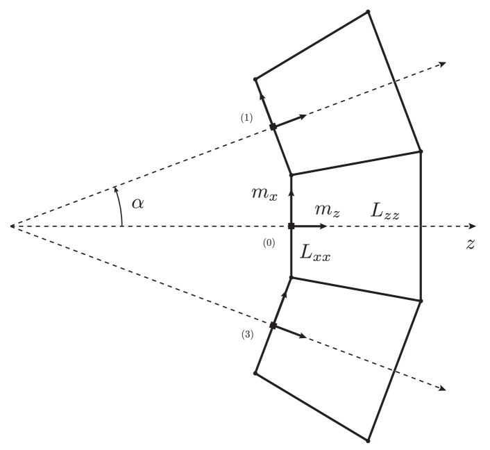
Figure 3: This shows an $xz$ section of the lattice obtained by cloning the original 2-dimensional lattice. The data in the upper and lower cells are identical to that in the middle cell, this follows from spherical symmetry. The small squares denote the central vertices of each computational cell. The angle $\alpha$ can be computed using standard Euclidean trigonometry as described in the text.

This pair of equations contains 4 spatial derivatives each of which we will estimate by a finite difference approximation. But in order to do so we must first have a sampling of the 4 curvatures at a cluster of points near and around the central vertex. Our simple ladder-like lattice, with its collection of computational cells along one radial axis, would allow us to compute only the $z$ partial derivatives. For the $x$ and $y$ derivatives we will need to extend the lattice along the $x$ and $y$ axes. In short we need a truly 3 dimensional lattice. Fortunately this is rather easy to do for this spacetime. We can use the spherical symmetry of the Schwarzschild spacetime to clone copies of the ladder (by spherical rotations) so that a typical central vertex of the parent ladder-lattice becomes surrounded by 4 copies of itself. It has two further nearby vertices, fore and aft along the radial axis, that are themselves central vertices of neighbouring cells in the original ladder-like lattice. In figure (3) we display an $xz$ slice of the cloned lattice.

We now need the coordinates of all six of the neighbouring vertices. This would require a solution of

$$L^{2}_{ij}=g_{\mu\nu}\left(x_{j}^{\mu}-x_{i}^{\mu}\right)\left(x_{j}^{\nu}-x_{i}^{\nu}\right)-\frac{1}{3}R_{\mu\alpha\nu\beta}x^{\mu}_{i}x^{\nu}_{i}x^{\alpha}_{j}x^{\beta}_{j}+\mathcal{O}\left(L^{5}\right)$$ (A.3)

for the $x^{\mu}_{i}$ for given values for the $L_{ij}$ and $R_{\mu\alpha\nu\beta}$. However, as we are only going to use these coordinates to construct transformation matrices which will in turn multiply the Riemann curvatures, it is sufficient to solve (A.3) using a flat metric. Note that the above equations can only be used to compute (in fact estimate) the spatial coordinates of the vertices. For the time coordinates we can appeal to the smoothness of the underlying metric to argue that for each vertex $t=\mathcal{O}\left(L^{2}\right)$. The result is that the typical central vertex, with coordinates $(0,0,0,0)$, will have 6 neighbouring central vertices with coordinates as per Table (1).

	Vertex		$t$	$x$	$y$	$z$
	0		( $0$ ,	$0$ ,	$0$ ,	$0$ )
	1		( $0$ ,	$L_{xx}$ ,	$0$ ,	$0$ )
	2		( $0$ ,	$0$ ,	$L_{yy}$ ,	$0$ )
	3		( $0$ ,	$-L_{xx}$ ,	$0$ ,	$0$ )
	4		( $0$ ,	$0$ ,	$-L_{yy}$ ,	$0$ )
	5		( $0$ ,	$0$ ,	$0$ ,	$L_{zz}$ )
	6		( $0$ ,	$0$ ,	$0$ ,	$-L_{zz}$ )

Table 1: Riemann normal coordinates, to $\mathcal{O}\left(L^{2}\right)$, of the central vertex and its 6 immediate neighbours. These coordinates were computed using a flat space approximation.

This accounts for the structure of our lattice but what values should we assign to the curvatures at the newly created vertices? Let $(A)_{PQ}$ denote the value of a quantity $A$ at the vertex $P$ in the local Riemann normal frame for vertex $Q$. Since our spacetime is spherically symmetric we can assert that

$$(A)_{00}=(A)_{11}=(A)_{22}=(A)_{33}=(A)_{44}$$

Then the idea that we will import data from neighbouring cells can be expressed as

$$(A)_{PQ}=(U)_{PQ}(A_{PP})$$

where $(U)_{PQ}$ is the transformation matrix, evaluated at $P$, from the Riemann normal frame of $P$ to that of $Q$. This matrix will be composed of spatial rotations and boosts.

To get the correct estimates for the first partial derivatives we need only compute $U$ to terms linear in the leg-lengths.

As an example, let us suppose we wished to compute $v^{\mu}{}_{,x}$ for a spherically symmetric vector field $v$ on the lattice. We start with $(v)_{10}=(U)_{10}(v)_{11}$ and

$$(U)_{10}=(B)_{10}(R)_{10}$$

where $(R)_{10}$ represents a rotation in the $x-y$ plane and $(B)_{10}$ a boost in the $t-x$ plane. Note that as we are working only to linear terms in the lattice scale the order in which we perform the rotation and boost does not matter. Thus we have

$$(R)_{10} =\begin{bmatrix}1&0&0&0\\ 0&\phantom{-}\cos\alpha&\sin\alpha&0\\ 0&-\sin\alpha&\cos\alpha&0\\ 0&0&0&1\end{bmatrix}$$

$$(B)_{10} =\begin{bmatrix}\cosh\beta&\sinh\beta&0&0\\ \sinh\beta&\cosh\beta&0&0\\ 0&0&1&0\\ 0&0&0&1\end{bmatrix}$$

The columns in the above matrices are labelled $(t,x,y,z)$ from left to right and likewise for the rows. As we will latter be forming products of these matrices with the curvatures it is sufficient to compute these matrices as if we were working in flat spacetime. Thus to leading order in the lattice spacing we find

$$\cos\alpha=1+\mathcal{O}\left(L^{3}\right)\>,\quad\sin\alpha=\frac{dL_{xx}}{dz}+\mathcal{O}\left(L^{2}\right)$$

$$\cosh\beta=1+\mathcal{O}\left(L^{3}\right)\>,\quad\sinh\beta=-K_{xx}L_{xx}+\mathcal{O}\left(L^{2}\right)$$

and thus

$$(U)_{10}=(B)_{10}(R)_{10}=\begin{bmatrix}1&-\displaystyle K_{xx}L_{xx}&0&0\\[5.0pt] -\displaystyle K_{xx}L_{xx}&1&0&\displaystyle\frac{dL_{xx}}{dz}\\[10.0pt] 0&0&1&0\\[5.0pt] 0&-\displaystyle\frac{dL_{xx}}{dz}&0&1\end{bmatrix}+\mathcal{O}\left(L^{2}\right)$$

In a similar manner we find

$$(U)_{20}=(B)_{20}(R)_{20}=\begin{bmatrix}1&0&-\displaystyle K_{yy}L_{yy}&0\\[5.0pt] 0&1&0&0\\[10.0pt] -\displaystyle K_{yy}L_{yy}&0&1&\displaystyle\frac{dL_{yy}}{dz}\\[5.0pt] 0&0&-\displaystyle\frac{dL_{yy}}{dz}&1\end{bmatrix}+\mathcal{O}\left(L^{2}\right)$$

$$(U)_{30}=(B)_{30}(R)_{30}=\begin{bmatrix}1&\displaystyle K_{xx}L_{xx}&0&0\\[5.0pt] \displaystyle K_{xx}L_{xx}&1&0&-\displaystyle\frac{dL_{xx}}{dz}\\[10.0pt] 0&0&1&0\\[5.0pt] 0&\displaystyle\frac{dL_{xx}}{dz}&0&1\end{bmatrix}+\mathcal{O}\left(L^{2}\right)$$

$$(U)_{40}=(B)_{40}(R)_{40}=\begin{bmatrix}1&0&\displaystyle K_{yy}L_{yy}&0\\[5.0pt] 0&1&0&0\\[10.0pt] \displaystyle K_{yy}L_{yy}&0&1&-\displaystyle\frac{dL_{yy}}{dz}\\[5.0pt] 0&0&\displaystyle\frac{dL_{yy}}{dz}&1\end{bmatrix}+\mathcal{O}\left(L^{2}\right)$$

For the remaining two matrices, $(U)_{50}$ and $(U)_{60}$, the job is quite simple, these matrices are built solely on boosts. This leads to

$$(U)_{50}=(B)_{50}(R)_{50}=\begin{bmatrix}1&0&0&-\displaystyle K_{zz}L_{zz}\\[5.0pt] 0&1&0&0\\[10.0pt] 0&0&1&0\\[5.0pt] -\displaystyle K_{zz}L_{zz}&0&0&1\end{bmatrix}+\mathcal{O}\left(L^{2}\right)$$

$$(U)_{60}=(B)_{60}(R)_{60}=\begin{bmatrix}1&0&0&\displaystyle K_{zz}L_{zz}\\[5.0pt] 0&1&0&0\\[10.0pt] 0&0&1&0\\[5.0pt] \displaystyle K_{zz}L_{zz}&0&0&1\end{bmatrix}+\mathcal{O}\left(L^{2}\right)$$

Returning now to the construction of $(v)_{10}$, we have

$$(v^{\mu})_{10} =(U^{\mu}{}_{\nu})_{10}(v^{\nu})_{11}$$

$$=(v^{\mu})_{11}+\left[-\displaystyle K_{xx}L_{xx}v^{x},-\displaystyle K_{xx}L_{xx}v^{t}+\displaystyle\frac{dL_{xx}}{dz}v^{z},0,-\displaystyle\frac{dL_{xx}}{dz}v^{x}\right]^{\mu}_{11}$$

and

$$(v^{\mu})_{30} =(U^{\mu}{}_{\nu})_{30}(v^{\nu})_{33}$$

$$=(v^{\mu})_{33}+\left[\displaystyle K_{xx}L_{xx}v^{x},\displaystyle K_{xx}L_{xx}v^{t}-\displaystyle\frac{dL_{xx}}{dz}v^{z},0,\displaystyle\frac{dL_{xx}}{dz}v^{x}\right]^{\mu}_{33}$$

We are now in a position to finally compute $(v^{t}_{,x})_{00}$, to wit

$$(v^{t}_{,x})_{00} =\frac{(v^{t})_{10}-(v^{t})_{30}}{2L_{xx}}+\mathcal{O}\left(L^{a}\right)$$

$$=\frac{(v^{t})_{11}-(v^{t})_{33}}{2L_{xx}}-K_{xx}\frac{(v^{x})_{11}+(v^{x})_{33}}{2}+\mathcal{O}\left(L^{a}\right)$$

Here we have written the truncation errors as $\mathcal{O}\left(L^{a}\right)$ with $a>0$ for it is not clear, at this level of analysis, what the exact nature of this term is (save that it vanishes as $L\rightarrow 0$). Since our spacetime is spherically symmetric we have

$$(v)_{00}=(v)_{11}=(v)_{22}=(v)_{33}=(v)_{44}$$

and thus

$$(v^{t}_{,x})_{00}=-K_{xx}(v^{x})_{00}+\mathcal{O}\left(L^{a}\right)$$

Similar calculations can be used to compute all of the spatial derivatives of $v^{\mu}$ at the central vertex.

We can now return to the principle objective of this section – to compute the various partial derivatives of the curvatures. We proceed exactly as above but with a minor change in that we will no longer carry the truncation errors within the calculations. Thus we have

$$(R_{\mu\alpha\nu\beta})_{i0}=(U_{\mu}{}^{\tau})_{i0}(U_{\alpha}{}^{\rho})_{i0}(U_{\nu}{}^{\delta})_{i0}(U_{\beta}{}^{\lambda})_{i0}(R_{\tau\rho\delta\lambda})_{ii}$$

for $i=1,2,3,4,5,6$ and $(U_{\mu}{}^{\nu})_{i0}=g_{\mu\rho}g^{\nu\tau}(U^{\rho}{}_{\tau})_{i0}$ with $g_{\mu\nu}={\rm diag}(-1,1,1,1)$. And, as before,

$$(R_{\mu\alpha\nu\beta})_{00}=(R_{\mu\alpha\nu\beta})_{11}=(R_{\mu\alpha\nu\beta})_{22}=(R_{\mu\alpha\nu\beta})_{33}=(R_{\mu\alpha\nu\beta})_{44}$$

due to spherical symmetry.

Using the above expressions for the $(U)_{i0}$ and the following finite difference approximations

$$(R_{tyxy,x})_{00} =\frac{(R_{tyxy})_{10}-(R_{tyxy})_{30}}{2L_{xx}}$$

$$(R_{txxy,y})_{00} =\frac{(R_{txxy})_{20}-(R_{txxy})_{40}}{2L_{yy}}$$

$$(R_{tzxz,x})_{00} =\frac{(R_{tzxz})_{10}-(R_{tzxz})_{30}}{2L_{xx}}$$

$$(R_{txxz,z})_{00} =\frac{(R_{txxz})_{50}-(R_{txxz})_{60}}{2L_{zz}}$$

we find that

$$R_{tyxy,x} =\phantom{-}K_{xx}\left(R_{xyxy}+R_{tyty}\right)+\frac{1}{L_{xx}}\frac{dL_{xx}}{dz}R_{tyyz}$$ (A.4)

$$R_{txxy,y} =-K_{yy}\left(R_{xyxy}+R_{txtx}\right)-\frac{1}{L_{yy}}\frac{dL_{yy}}{dz}R_{txxz}$$ (A.5)

$$R_{tzxz,x} =\phantom{-}K_{xx}\left(R_{xzxz}+R_{tztz}\right)+\frac{1}{L_{xx}}\frac{dL_{xx}}{dz}R_{txxz}$$ (A.6)

$$R_{txxz,z} =-K_{zz}\left(R_{xzxz}+R_{txtx}\right)$$ (A.7)

We have dropped the $00$ subscript as we no longer need to distinguish between the neighbouring frames. By spherical symmetry we have

$$L_{xx}=L_{yy}\>,\quad K_{xx}=K_{yy}\>,\quad R_{txxz}=R_{tyyz}\>,\quad R_{xzxz}=R_{yzyz}$$

while from the vacuum Einstein equations we have

$$0 =R_{tz}=-R_{txxz}-R_{tyyz}$$

$$0 =R_{xx}=R_{xyxy}+R_{xzxz}-R_{txtx}$$

$$0 =R_{yy}=R_{xyxy}+R_{yzyz}-R_{tyty}$$

$$0 =R_{zz}=R_{xzxz}+R_{yzyz}-R_{tztz}$$

Combining the last few equations leads to

$$R_{txtx}=R_{tyty}=R_{xyxy}+R_{xzxz}$$

$$R_{txxz}=R_{tyyz}=0\>,\quad R_{tztz}=2R_{xzxz}$$

Substituting these into the above equations (A.4–A.7) and subsequently into the previous expressions for the Bianchi identities (A.1,A.2) leads to the following pair of equations

$$\frac{dR_{xyxy}}{dt} =2K_{xx}\left(2R_{xyxy}+R_{xzxz}\right)$$

$$\frac{dR_{xzxz}}{dt} =3K_{xx}R_{xzxz}+K_{zz}\left(R_{xyxy}+2R_{xzxz}\right)$$

Our job is almost complete, but we still have two tasks ahead of us i) to introduce a lapse function and ii) to account for the limited time interval over which a single Riemann normal frame can be used. The first task is rather easy, we simply make the coordinate substitution $t\rightarrow Nt$ leading to

$$\frac{dR_{xyxy}}{dt} =2NK_{xx}\left(2R_{xyxy}+R_{xzxz}\right)$$ (A.8)

$$\frac{dR_{xzxz}}{dt} =3NK_{xx}R_{xzxz}+NK_{zz}\left(R_{xyxy}+2R_{xzxz}\right)$$ (A.9)

and where we now have $(g_{\mu\nu})_{o}={\rm diag}(-N^{2},1,1,1)$. The lapse $N$ can be freely chosen at each vertex of the lattice (but subject to the obvious constraint that $N>0$). The second task is a bit more involved. We know that each Riemann normal frame is limited in both space and time. Thus no single Riemann normal frame can be used to track the evolution for an extended period of time. We will have no choice but to jump periodically to a new frame. This can be elegantly handled in the moving frame formalism. Thus our task reduces to finding a new set of evolution equations for the frame components ${\cal R}_{xyxy}$ and ${\cal R}_{xzxz}$ based on the equations given above for $R_{xyxy}$ and $R_{xzxz}$.

Let $e^{\mu}{}_{a}$, $a=t,x,y,z$ be an orthonormal tetrad, tied to the worldline of the central vertex and aligned to the coordinate axes. Thus we have $e^{\mu}{}_{t}$ as the future pointing tangent vector to the worldline while $e^{\mu}{}_{z}$ points along the $z$-axis. Then

$$\frac{d{\cal R}_{xyxy}}{dt}= \frac{d}{dt}\left(R_{\mu\alpha\nu\beta}e^{\mu}{}_{x}e^{\alpha}{}_{y}e^{\nu}{}_{x}e^{\beta}{}_{y}\right)$$

$$\frac{d{\cal R}_{xzxz}}{dt}= \frac{d}{dt}\left(R_{\mu\alpha\nu\beta}e^{\mu}{}_{x}e^{\alpha}{}_{z}e^{\nu}{}_{x}e^{\beta}{}_{z}\right)$$

Since our spacetime is spherically symmetric it is not hard to see that the tetrads of two consecutive cells (on the vertex worldline) are related by a boost in the $t-z$ plane (arising from gradients in the lapse function). A simple calculation shows that

$$\frac{de^{\mu}{}_{x}}{dt}=0\>,\quad\frac{de^{\mu}{}_{y}}{dt}=0\>,\quad\frac{de^{\mu}{}_{t}}{dt}=N_{,z}e^{\mu}{}_{z}\>,\quad\frac{de^{\mu}{}_{z}}{dt}=N_{,z}e^{\mu}{}_{t}$$

which when combined with the above leads to

$$\frac{d{\cal R}_{xyxy}}{dt}= \left(\frac{dR_{\mu\alpha\nu\beta}}{dt}\right)e^{\mu}{}_{x}e^{\alpha}{}_{y}e^{\nu}{}_{x}e^{\beta}{}_{y}$$ (A.10)

$$\frac{d{\cal R}_{xzxz}}{dt}= \left(\frac{dR_{\mu\alpha\nu\beta}}{dt}\right)e^{\mu}{}_{x}e^{\alpha}{}_{z}e^{\nu}{}_{x}e^{\beta}{}_{z}-2\frac{N_{,z}}{N}R_{\mu\alpha\nu\beta}e^{\mu}{}_{t}e^{\alpha}{}_{x}e^{\nu}{}_{x}e^{\beta}{}_{z}$$ (A.11)

In our frame we have chosen $\left(g_{\mu\nu}\right)_{o}={\rm diag}(-N^{2},1,1,1)$, $e^{\mu}{}_{a}=\delta^{\mu}_{a}$ for $a=x,y,z$ and $e^{\mu}{}_{t}=1/N$, thus we see that the last term in the previous equation is proportional to ${\cal R}_{txxz}$. But for the Schwarzschild spacetime we know that ${\cal R}_{txxz}=0$ and thus we have

$$\frac{d{\cal R}_{xyxy}}{dt}= \left(\frac{dR_{\mu\alpha\nu\beta}}{dt}\right)e^{\mu}{}_{x}e^{\alpha}{}_{y}e^{\nu}{}_{x}e^{\beta}{}_{y}$$ (A.12)

$$\frac{d{\cal R}_{xzxz}}{dt}= \left(\frac{dR_{\mu\alpha\nu\beta}}{dt}\right)e^{\mu}{}_{x}e^{\alpha}{}_{z}e^{\nu}{}_{x}e^{\beta}{}_{z}$$ (A.13)

which, when combined with (A.8,A.9), leads immediately to the evolution equations (4.7,4.8) quoted in section (4).

Figure 4: The Schwarzschild areal coordinate $r$ and the lattice $L_{xx}$ at the throat are related by $r(t)=2mL_{xx}(t)/L_{xx}(0)$. In geodesic slicing $r(t)$ at the throat is described by the parametric equations $r(t)=m(1+\cos\eta(t))$, $t(\eta)=m(\eta+\sin\eta)$. These equations allow us to plot the exact evolution of $r(t)$ (the smooth curve) against estimates from the lattice (solid points). The relative errors are seen to be very small and are dominated by the truncation errors in the Runge-Kutta scheme.

Figure 8: In the absence of gravitational radiation the area of the horizon should remain constant. It follows that the $L_{xx}$ should be constant on the horizon. Here we plot the fractional variation of $L_{xx}$ on the horizon. The irregular behaviour of the plots for later times is due, in part, to the difficulty in accurately locating the horizon.

References

- [1] F. Pretorius, Evolution of binary black hole spacetimes, Phys. Rev. Lett. 95 (2005) 121101, gr-qc/0507014.
- [2] M. Campanelli, C. O. Lousto, P. Marronetti, and Y. Zlochower, Accurate Evolutions of Orbiting Black-Hole Binaries without Excision, Phys.Rev.Lett. 96 (2006) no. 111101, .
- [3] J. G. Baker, J. Centrella, D.-I. Choi, M. Koppitz, and J. van Meter, Gravitational-Wave Extraction from an Inspiraling Configuration of Merging Black Holes, Phys.Rev.Lett. 96 (2006) no. 111102, .
- [4] O. A. Reula. Hyperbolic Methods for Einstein’s Equations. http://www.livingreviews.org/lrr-1998-3.
- [5] H. Friedrich, Hyperbolic reductions for Einstein’s equations, Class. Quantum Grav. 13 (1996) 1451–1469.
- [6] A. Anderson and J. W. York, Jr., Fixing Einstein’s Equations, Phys. Rev. Lett. 82 (1999) 4384–4387.
- [7] F. B. Estabrook, R. S. Robinson, and H. D. Wahlquist, Hyperbolic equations for vacuum gravity using special orthonormal frames, Class. Quantum Grav. 14 (1997) 1237–1247.
- [8] H. van Elst and C. Uggla, General relativistic 1 + 3 orthonormal frame approach, Class. Quantum Grav. 14 (1997) 2673–2695.
- [9] R. T. Jantzen, P. Carini, and D. Bini. GEM: the User Manual, Understanding Spacetime Splittings and Their Relationships. http://www34.homepage.villanova.edu/robert.jantzen/gem/.
- [10] M. H. P. M. van Putten and D. M. Eardley, Nonlinear wave equations for relativity, Phys. Rev. D 53 (1996) 3056–3063.
- [11] M. H. P. M. van Putten, Numerical integration of nonlinear wave equations for general relativity, Phys. Rev. D 55 (1997) 4705–4711.
- [12] L. Brewin and J. Kajtar, (Paper 1) A Smooth Lattice construction of the Oppenheimer-Snyder spacetime, Phys. Rev. D 80 (2009) 104004, arXiv:0903.5367. http://users.monash.edu.au/~leo/research/papers/files/lcb09-05.html.
- [13] L. Brewin, (Paper 2) Deriving the ADM 3+1 evolution equations from the second variation of arc length, Phys. Rev. D 80 (2009) 084030, arXiv:0903.5365. http://users.monash.edu.au/~leo/research/papers/files/lcb09-04.html.
- [14] L. Brewin, Long term stable integration of a maximally sliced Schwarzschild black hole using a smooth lattice method, Class. Quantum Grav. 19 (2002) 429–455.
- [15] L. Brewin, An ADM 3+1 formulation for smooth lattice general relativity, Class. Quantum Grav. 15 (1998) 2427–2449.
- [16] D. Bernstein, D. Hobill, and L. Smarr, Black hole spacetimes: testing numerical relativity, in Frontiers in numerical relativity, C. R. Evans, L. S. Finn, and D. W. Hobill, eds., pp. 57–73. Cambridge University Press, Cambridge., 1989.
- [17] R. Beig and N. Ó. Murchadha, Late time behavior of the maximal slicing of the Schwarzschild black hole, Phys. Rev. D 57 (1998) no. 8, 4728–4737.
- [18] L. Brewin, Riemann Normal Coordinate expansions using Cadabra, Class. Quantum Grav. 26 (2009) 175017, arXiv:0903.2087. http://users.monash.edu.au/~leo/research/papers/files/lcb09-03.html.