Gravitational sources induced by exotic smoothness

Abstract

In this paper we construct a coordinate atlas in an exotic $\mathbb{R}^{4}$ using Bizaca’s construction. The main source for such an atlas is the handle body decomposition of a Casson handle, which of course is an infinite, but periodic, process. The immersion of the end-periodic manifold into $\mathbb{R}^{4}$ is directly related to the exoticness of the $\mathbb{R}^{4}$ and also gives rise naturally to a spinor field. Thus we obtain the interesting result that the simplest exotic $\mathbb{R}^{4}$ generates an extra spinor field by exoticness.

1 Introduction

The existence of exotic (non-standard) smoothness on topologically simple 4-manifolds such as exotic $\mathbb{R}^{4}$ or $S^{3}\times\mathbb{R},$ has been known since the early eighties but the use of them in physical theories has been seriously hampered by the absence of finite coordinate presentations. However, the work of Bizaca and Gompf BizGom:96 provides a handle body representation of an exotic $\mathbb{R}^{4}$ which can serve as an infinite, but periodic, coordinate representation.

Thus we are looking for the decomposition of manifolds into small non-trivial, easily controlled objects (like handles). As an example consider the 2-torus $T^{2}=S^{1}\times S^{1}$ usually covered by at least 4 charts. However, it can be also decomposed using two 1-handles $D^{1}\times D^{1}$ attached to the $0-$handle $D^{0}\times D^{2}=D^{2}$ along their boundary $\partial D^{2}=S^{1}$ via the boundary component of the 1-handle $\partial D^{1}\times D^{1}=S^{0}\times D^{1}$, the disjoint uinon of two lines $S^{0}\times D^{1}=D^{1}\sqcup D^{1}$. Finally one has to add a 2-handle $D^{2}\times D^{0}$ to get the closed manifold $T^{2}$. Every 1-handle can be covered by (at least) two charts and finally we recover the covering by 4 charts. Both pictures are equivalent but the handle picture has one simple advantage: it reduces the number of fundamental pieces of a manifold and of the transition maps. The gluing maps of the handles can be seen as a generalization of transition maps. Then the handle picture presents only the most important of these gluing or transition maps, omitting the trivial transition maps.

In this paper we will present such a coordinate representation, albeit infinite, of an exotic $\mathbb{R}^{4}$ based on the handle body decomposition of Bizaca and Gompf. We suggest that one of the consequences of this approach would be to suggest a positive answer for the Brans conjecture, that exotic smoothness serves as an additional gravitational source as a spinor field naturally arising from the handlebody construction. The compact case was worked out in AsselmeyerRose2010 .

2 Construction of exotic $\mathbb{R}^{4}$

Our model of space-time is the non-compact space topological $\mathbb{R}^{4}$. The results can be easily generalized for other cases such as $S^{3}\times\mathbb{R}$.

2.1 Handle decomposition and Casson handle

Every 4-manifold can be decomposed using standard pieces such as $D^{k}\times D^{4-k}$, the so-called $k$-handle attached along $\partial D^{k}\times D^{4-k}$ to the $0-$handle $D^{0}\times D^{4}=D^{4}$. In the following we need two possible cases: the 1-handle $D^{1}\times D^{3}$ and the 2-handle $D^{2}\times D^{2}$. These handles are attached along their boundary components $S^{0}\times D^{3}$ or $S^{1}\times D^{2}$ to the boundary $S^{3}$ of the $0-$handle $D^{4}$ (see GomSti:1999 ). The attachment of a 2-handle is defined by a map $S^{1}\times D^{2}\to S^{3}$, the embedding of a circle $S^{1}$ into the 3-sphere $S^{3}$, i.e. a knot. This knot into $S^{3}$ can be thickened (or a knotted solid torus). The important fact for our purposes is the freedom to twist this knotted solid torus via Dehn twist. The (integer) number of these twists (with respect to the orientation) is called the framing number or the framing. Thus the gluing of the 2-handle on $D^{4}$ can be represented by a knot or link together with an integer framing. The simplest example is the unknot with framing $\pm 1$ is the complex projective space $\mathbb{C}P^{2}$ or with reversed orientation $\overline{\mathbb{C}P}^{2}$, respectively.

The 1-handle will be glued by the map of $S^{0}\times D^{3}\to S^{3}$ represented by two disjoint solid 2-spheres $D^{3}$. Akbulut AkbKir:79 introduced another description. He observed that a 1-handle is something like a surgered 2-handle with a fixed framing. The notation in this figure represents erasing the framing coefficient of the unknot by putting a dot on it (see figure 1). We remark that some of the figures are a redrawing of pictures in GomSti:1999 .

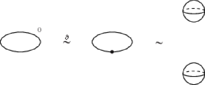
Figure 1: Surgering a 2-handle to a 1-handle (The symbol $\partial$ indicates the diffeomorphism between the boundaries of the corresponding 4-manifolds)

In detail, the procedure can be described as follows. The main observation is that the union of one 0-handle and $m$ 1-handles ($\approx\natural_{m}S^{1}\times D^{3}$ with $\natural_{m}$ as $m$-times boundary connected sum, see appendix A) has the same boundary as $m$ 2-handles (0-framed) ($\approx\natural_{m}S^{2}\times D^{2}$) to an $m$-component unlink (i.e., the boundary of an embedding in $S^{3}$ of $m$ disjoint disks). In fact, the latter 4-manifold contains a canonical collection of $m$ (uniquely) framed 2-spheres $S^{2}\times\{*\}\subset S^{2}\times D^{2}$, and surgery on these framed spheres gives back $\natural_{m}S^{1}\times D^{3}$. Thus, an $m$-component unlink with a dot on each component is the same as $m$ 1-handles.

Now we are ready to present the handle body decomposition of an exotic $\mathbb{R}^{4}$ by Bizaca in Fig. 2.

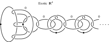
Figure 2: Handle decomposition of Bizacas exotic $\mathbb{R}^{4}$

It is very important to notice that the exotic $\mathbb{R}^{4}$ is the interior of the given handle body (since the handle body has a non-null boundary). The construction can be divided into two parts represented in the figure 3.

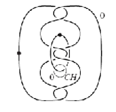
Figure 3: Principal picture of an exotic $\mathbb{R}^{4}$

The first part is known as the Akbulut cork represented by figure 4.

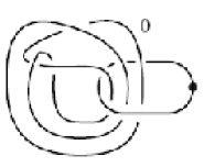
Figure 4: Akbulut cork

In the appendix B we will give a short description of the Akbulut cork and its meaning for the smoothness of 4-manifolds. The second part is the Casson handle $CH$ where we use the simplest example (see figure 5).

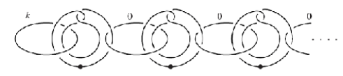
Figure 5: Simplest Casson handle

Start with the construction of the Akbulut cork $A$ as a contractible 4-manifold with boundary the homology 3-sphere $\Sigma(2,5,7)$. This homology 3-sphere is given by the set

$$\Sigma(2,5,7)=\left\{x,y,z\in\mathbb{C}\,|\,x^{2}+y^{5}+z^{7}=0\,,\,|x|^{2}+|y|^{2}+|z|^{2}=1\right\}$$

Now it is easy to define the interior $int(A)$ of the cork as the set

$$int(A)=\left\{x,y,z\in\mathbb{C}\,|\,x^{2}+y^{5}+z^{7}=0\,,\,|x|^{2}+|y|^{2}+|z|^{2}<1\right\}$$

This set is a smooth manifold which can be covered by a finite number of charts. But the smoothness structure of the exotic $\mathbb{R}^{4}$ depends mostly on the Casson handle. If we take (instead of the simplest handle in Fig.5) the more complex Casson handle in Fig. 6 then we obtain another exotic $\mathbb{R}^{4}$ non-diffeomorphic to the previous one.

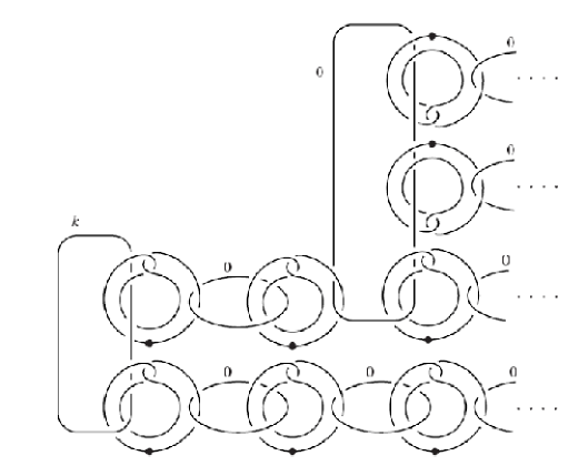
Figure 6: More complex Casson handle

Now consider the Casson handle and its construction in more detail. Briefly, a Casson handle $CH$ is the result of attempts to embed a disk $D^{2}$ into a 4-manifold. In most cases this attempt fails and Casson Cas:73 looked for a substitute, which is now called a Casson handle. Freedman Fre:82 showed that every Casson handle $CH$ is homeomorphic to the open 2-handle $D^{2}\times\mathbb{R}^{2}$ but in nearly all cases it is not diffeomorphic to the standard handle Gom:84 ; Gom:89 . The Casson handle is built by iteration, starting from an immersed disk in some 4-manifold $M$, i.e. a map $D^{2}\to M$ with injective differential. Every immersion $D^{2}\to M$ is an embedding except on a countable set of points, the double points. One can kill one double point by immersing another disk into that point. These disks form the first stage of the Casson handle. By iteration one can produce the other stages. Finally consider not the immersed disk but rather a tubular neighborhood $D^{2}\times D^{2}$ of the immersed disk including each stage. The union of all neighborhoods of all stages is the Casson handle $CH$. So, there are two input data involved with the construction of a $CH$: the number of double points in each stage and their orientation $\pm$. Thus we can visualize the Casson handle $CH$ by a tree: the root is the immersion $D^{2}\to M$ with $k$ double points, the first stage forms the next level of the tree with $k$ vertices connected with the root by edges etc. The edges are evaluated using the orientation $\pm$. Every Casson handle can be represented by such an infinite tree. The Casson handle $CH(R_{+})$ in Fig.5 is the simplest Casson handle represented by the simplest tree $R_{+}$ having one vertex in each level connected by one edge with evaluation $+$. We will now go into more detail. The reader not interested in very technical terms can go directly to the next subsection.

Each building block of a Casson handle, sometimes called a “kinky” handle, is diffeomorphic to $\natural(S^{1}D^{3})$ with two attaching regions. Technically speaking, one region is a tubular neighborhood of band sums of Whitehead links (see Fig. 7) connected with the previous block.

Figure 7: Whitehead link

The other region is a disjoint union of the standard open subsets $S^{1}\times D^{2}$ in $\#S^{1}\times S^{2}=\partial(\natural S^{1}D^{3})$ (this is connected with the next block). The number of end-connected sums is exactly the number of self intersections of the immersed two handle. The simplest Casson handles have $S^{1}\times D^{3}$ as their building blocks represented by the Fig. 7.

We attach a Casson handle to the zero–handle along the attaching circle and denote it by $S=D^{4}\cup CH$. Consider a simple Casson handle, say $CH(R_{+})$, a periodic Casson handle with positive orientation kinks (see Fig. 5). As shown in Kato2004 , the Casson handle is a so-called end-periodic manifold, i.e. a manifold with a periodic structure of building blocks, discussed in the next subsection. The periodicity of the topological construction can be naturally translated into the periodicity of the metric to be imposed on the resulting manifold. The building block as an open manifold becomes an ‘open cylindrical’ manifold. Then one connects two attaching regions in a block. The result becomes a cylindrical manifold on which analysis is already well known. By equipping it with a suitable weight function, one will apply the generalized Fourier–Laplace transform between complex functions on the cylindrical manifold and its periodic cover. Thus one is able to construct operators or functions over $S=D^{4}\cup CH(R(2))$. This method shows that once one obtains some suitable function spaces on any open manifolds, then the generalized Fourier–Laplace transform (described below) works on their periodic covers. We will use this observation iteratively. As described above a Casson handle can be expressed by an infinite tree with one end point and with a sign $\pm$ on each edge. The next simplest Casson handle (see Fig. 6) will be represented as follows (here we will follow Kato2004 very closely). Let $R_{+}$ be the half-line with the vertices $\left\{0,1,2,\ldots\right\}$. We prepare another family of half-lines $\left\{R_{+}^{i}\right\}_{i=1,2,...}$ assigned with indices. Then we obtain another infinite tree:

$$R(2)=R_{+}\bigcup_{i=1,2,\ldots}R_{+}^{i}$$

where we connect $i$ in $R_{+}$ with $0$ in $R_{+}^{i}$. For example one may assign $-$ on $R_{+}$ and $+$ on all $\left\{R_{+}^{i}\right\}_{i}$. Then one obtains the corresponding Casson handle $CH(R(2))$. In this case the building blocks are diffeomorphic to $\hat{\Sigma}_{2}=(S^{1}\times D^{3})\natural(S^{1}\times D^{3})$ along $R_{+}$. $\hat{\Sigma}_{2}$ has three attaching components. One is $\mu$, the tubular neighborhood of the band sum of two Whitehead links as before. We will denote the others by $\mu^{\prime}$ and $\gamma$ , where these represent a generator of $\pi_{1}\left(\hat{\Sigma}_{2}\right)$. In order to apply Fourier–Laplace transform (described below), one takes end-connected sums twice. Firstly one takes the end-connected sum between $\mu$ and $\mu^{\prime}$ as before. The result is an ‘open cylindrical’ manifold, since there still remains one attaching region, $\gamma$ . One takes the end-connected sum of this with $CH(R_{+})$ along $\gamma$ . In this manner, one obtains another open manifold, $\left(\hat{\Sigma}_{2}/\left(\mu\sim\mu^{\prime}\right)\right)\natural_{\gamma}CH(R_{+})$. Thus one is again able to construct operators or functions over $S=D^{4}\cup CH(R(2))$.

2.2 The periodic coordinate patch

By using the interpretation of the previous subsection Kato2004 , the Casson handle can be interpreted as an end-periodic manifold. An end-periodic manifold starts with a compact submanifold, $K,$ with boundary or end $N$ and building blocks $W$ with two ends. Now we glue the building blocks along a chain to obtain an end-periodic manifold. In the case of the Casson handle, the compact $K$ is the Akbulut cork described above and the building block is the tubular neighborhood of the self-intersecting disk. In the following subsection we will describe the general approach to end-periodic manifolds and their analytical properties using extensively Taubes paper Tau:87 . Then we will discuss the special end-periodic manifold, the Casson handle. Finally the coordinate patch is given by the handle decomposition of the Casson handle.

2.2.1 Analytical properties of end-periodic manifolds

The following definition is very formal and we refer to the Fig. 8.

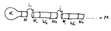
Figure 8: end-periodic manifold (fig. redraw from Tau:87 )

A smooth, oriented manifold $M$ is end-periodic if the following data exists (here we will follow Taubes paper Tau:87 very closely):

1. A smooth, connected, oriented and open manifold $W$ with two ends, $N_{+}$ and $N_{-}$. $W$ is called the fundamental segment or building block. Thus, there exists a compact set $C\subset W$ such that $W\setminus C$ is the disjoint union of two nonempty, connected, open sets, $N_{+}$ and $N_{-}$.

2. Suppose that there is a compact set $C_{+}\subset N_{+}$ such that $N_{+}\setminus C_{+}$ has two connected components, $N_{++}$ and $N_{+-}$. Assume that $C_{+}$ is such that $W\setminus C_{+}$ is the disjoint union of $N_{-}\cup C\cup N_{+-}$ and $N_{++}$. Similarly, assume that a compact set $C_{-}\subset N_{-}$exists such that $N_{-}\setminus C$ is the disjoint union of two connected components $N_{--}$and $N_{-+}$, and that $W\setminus C_{-}$ is the disjoint union of $N_{--}$ and $N_{-+}\cup C\cup N_{+}$. Assume that there is a diffeomorphism $i:N_{+}\to N_{-}$ which is orientation preserving and which takes $N_{++}$to $N_{-+}$ and $N_{+-}$ to $N_{--}$.

3. An open set $K\subset M$, with one end, $N$. Suppose that a compact set $C_{0}\subset N$ exists such that $N\setminus C_{0}$ is the disjoint union of two open sets $N_{0-}$and $N_{0+}$. Assume that $K\setminus C$ has two components, $\left(K\setminus N\right)\cup N_{0-}$ and $N_{0+}$. Require that there exists a diffeomorphism $i_{-}:N\to N_{-}$ which takes $N_{0-}$to $N_{--}$ and $N_{0+}$ to $N_{-+}$. Require that $i_{-}$ preserve orientation.

4. An orientation preserving diffeomorphism $\phi:M\to K\cup_{N}W\cup_{N}W\cup_{N}\cdots$ . Here $K\cup_{N}W$ is obtained from the disjoint union of $K$ and $W$ by identifying $N\subset K$ with $N_{-}\subset W$ via $i_{-}$. Also, $W\cup_{N}W$ is obtained from the disjoint union of two copies of $W$, $W_{1}\cup W_{2}$, by identifying $N_{+}\subset W$, with $N_{-}\subset W$, via $i_{-}$. (see Fig. 8)

In particular, there is an identifying map $T:W_{i}\to W_{i+1}$ of the copies of $W$. With the help of the map $T$ it is possible to investigate analytical properties of functions. We will follow very closely the article of Taubes Tau:87 for the analytical description of end-periodic manifolds.

First note that the map $i:N_{+}\to N_{-}$ can be used to identify the two ends of the building block $W$. One obtains $Y=W/i$ having the $\mathbb{Z}$-fold cover

$$\tilde{Y}=\cdots\cup_{N}W_{-1}\cup_{N}W_{0}\cup_{N}W_{1}\cup_{N}\cdots$$

as an end-periodic manifold with projection $\pi:\tilde{Y}\to Y$. Then the end

$$End(M)=W_{0}\cup_{N}W_{1}\cup_{N}W_{2}\cup_{N}\cdots$$ (1)

is a subset of $Y$ and can be identified with $M\setminus(K\setminus N)$. A vector bundle $E\to M$ is end-periodic if the the map $T$ lifts to a bundle map $\tilde{T}:E|_{W_{i}}\to E|_{W_{i+1}}$ or if $E|_{End(M)}=\pi^{*}E_{Y}$ where $E_{Y}\to Y$ is a vector bundle and $\pi:End(M)\to Y$ the projection. Then we obtain the main idea for the analytical description: Transform a function over $M$ to a function over $\tilde{Y}$ considered as periodic function. Thus, it is enough to consider a function as a smooth, compactly supported section $\psi\in\Gamma_{0}(\tilde{E})$ of a periodic vector bundle $\tilde{E}\to\tilde{Y}$. We define the generalized Fourier-Laplace transform (or Fourier-Laplace transform for short) of $\psi$ by

$$\hat{\psi}_{z}(.)=\sum_{n=-\infty}^{\infty}z^{n}(\tilde{T}^{n}\psi)(.)$$ (2)

with $z=\exp(i\delta)\in S^{1}=\mathbb{C}/\mathbb{Z}=\mathbb{C}^{*}$. $\hat{\psi}$ defines a smooth section of the vector bundle

$$E_{Y}(z)=\left[\tilde{E}\otimes\mathbb{C}/\mathbb{Z}\right]$$

over $Y=\tilde{Y}/\mathbb{Z}$, where $\mathbb{Z}$ acts on $\tilde{E}\otimes\mathbb{C}$ via the action sending $1\in\mathbb{Z}$ and $(p,\lambda)\in E\otimes\mathbb{C}$ to $(\tilde{T}p,\,z\lambda)$. The collection

$$E_{Y}=\left\{E_{Y}(z):z\in\mathbb{C}/\mathbb{Z}\right\}$$

can be seen as a smooth vector bundle over $Y\times\mathbb{C}/\mathbb{Z}$. The Fourier-Laplace transform can be inverted as follows: Let $\hat{\eta}$ be any section of $E_{Y}$ over $Y\times\mathbb{C}^{*}$ holomorphic in $\mathbb{C}^{*}=\mathbb{C}/\mathbb{Z}=S^{1}$. Then, if $s\in(0,\infty)$, the formula

$$(\tilde{T}^{n}\eta)(x)=\frac{1}{2\pi i}\intop_{|z|=s}z^{-n}\hat{\eta}_{z}(\pi(x))\frac{dz}{z}$$ (3)

for $x\in W_{0}$ and $\pi(x)\in Y$ defines a section of $\tilde{E}$ over $\tilde{Y}$.

2.2.2 The metric and the periodic coordinate patch

We are interested in a smooth metric $g$ over $M$ which can be seen as a section in the tensor bundle $TM\otimes TM$. One way to introduce a metric was described in Kato2004 by using an embedding of $M$ in some Euclidean space. Here we will use another method to construct $g$ by a periodic metric $\hat{g}$ on $Y$ giving a metric on the building block $W$. To reflect the number of the building block, we have to extend $\hat{g}$ to $Y\times\mathbb{C}^{*}$by using a metric $\hat{g}_{z}$holomorphic in $z\in\mathbb{C}^{*}=S^{1}$. From the formal point of view we have

$$\hat{g}_{z}(.)=\sum_{n=0}^{\infty}a_{n}z^{n}\cdot\hat{g}(.)$$ (4)

where the coefficient $a_{n}$ represents the building block $W_{n}$ in $End(M)$ (see (1)). Without loss of generality we can choose the coordinates $x$ in $M$ so that the $0$th component $x_{0}$ is related to the integer $n=[x_{0}]$ via its integer part $[\>]$. Using the inverse transformation (3) we can construct a smoth metric $g$ in $End(M)$ at the $n$th building block via

$$(\tilde{T}^{n}g)(x)=\frac{1}{2\pi i}\intop_{|z|=s}z^{-n}\hat{g}_{z}(\pi(x))\frac{dz}{z}$$

for $x\in End(M)\subset\tilde{Y}$, $s\in(0,\infty)$, $n=[x_{0}]$ and $\pi:\tilde{Y}\to Y$.

Let $g_{A}$ be the metric in the interior of the cork $A$. As discussed above the Casson handle can be interpreted as end-periodic manifold if the Casson handle is generated by a balanced tree. The two infinite trees $R_{\pm},R(2)$ in subsection 2.1 are examples of balanced trees. Using this information together with the handle body structure of the exotic $\mathbb{R}^{4}$ then we obtain for the metric $g$ on $M=\mathbb{R}_{\Theta}^{4}$:

$$g(x)=\begin{cases}g_{A}(x)&x\in int(A)\\ (\tilde{T}^{[x_{0}]}g)(x)&x\in End(M)\end{cases}$$

which is periodic at the end $End(M)$ of $M$. The end-periodic structure of the Casson handle induces the periodic coordinate patch of the exotic $\mathbb{R}^{4}$.

But can we make sense of the idea of localizing the exotic smoothness of the $\mathbb{R}_{\Theta}^{4}$? The work in Biz:95 ; BizGom:96 implies that the Casson handle relative to the attaching circle encoded in the periodic structure is the main incredient. Thus we have to analyze the structure of the Casson handle more carefully. The main ingredient of a Casson handle $CH$ is the immersed disk $D^{2}\hookrightarrow CH$, i.e. the image is a disk with self-intersections. In the appendix C we represent such a disk in appropriate coordinates. In the next section we will investigate this immersed disk representing the attaching circle of the Casson handle.

3 The Brans conjecture

For the following we assume a trivial Casson handle $CH_{0}=D^{2}\times\mathbb{R}^{2}$ in the standard $M=\mathbb{R}^{4}$ (i.e. having the standard differential structure) and a non-trivial Casson handle $CH$ in the exotic $N=\mathbb{R}_{\Theta}^{4}$ (i.e. admitting an exotic differential structure). We assume a metric $g_{M}$ on $M$ (constructed above) satisfying the source-free Einstein equation

$$R_{\mu\nu}=0\quad.$$ (5)

The corresponding action is

$$S=\intop_{M}R_{M}\sqrt{g_{M}}d^{4}x$$

with the scalar curvature $R_{M}$ of $M$. As stated above, the differential structure depends on the Casson handle $CH$ relative to the attaching region $\partial CH$. As Bizaca Biz:94 ; Biz:94a ; Biz:95 showed the Casson handle will be attached to the Akbulut cork $A$ defined above along a circle. Then the complements $M\setminus CH_{0}$ and $N\setminus CH$ are diffeomorphic. Thus, from the physical point of view we have the relative action

$$\intop_{M\setminus CH_{0}}R_{M}\sqrt{g_{M}}d^{4}x$$

but the manifold $M\setminus CH_{0}$ has a boundary $\partial CH_{0}$ and as we learned above the concrete embedding of this boundary (i.e. the attaching of the Casson handle) determines the differential structure. But then we need the action with a boundary term

$$S(M,CH_{0})=\intop_{M\setminus CH_{0}}R_{M}\sqrt{g_{M}}d^{4}x+\intop_{\partial(M\setminus CH_{0})}K_{CH_{0}}\sqrt{g_{\partial}}d^{3}x$$ (6)

where $K_{CH_{0}}$ is the trace of the second fundamental form of the boundary $\partial CH_{0}$ with metric $g_{\partial}$. Now we are looking for the motivation of the action at the boundary. As shown by York York1972 , the fixing of the conformal class of the spatial metric in the ADM formalism leads to a boundary term which can be also found in the work of Hawking and Gibbons GibHaw1977 . Also Ashtekar et.al. Ashtekar08 ; Ashtekar08a discussed the boundary term in the Palatini formalism. All these discussion suggest the choice of the following term for a boundary

$$\intop_{\partial(M\setminus CH_{0})}K_{CH_{0}}\sqrt{g_{\partial}}d^{3}x=\intop_{\partial(M\setminus CH_{0})}tr(\theta\wedge R)$$

by using a frame $\theta$ and the curvature 2-form $R$. The attaching region $\partial CH$ can be described as the immersion of $D^{2}\times(0,1)$ into $M=\mathbb{R}^{4}$. In appendix D we describe the spinor representation of an immersed surface $D^{2}$ in $\mathbb{R}^{3}$ which can be easily extended to an immersion of the attaching region $D^{2}\times(0,1)$ into $M=\mathbb{R}^{4}$. By using relation (15) in appendix D we obtain the contribution

$$\intop_{\partial(M\setminus CH_{0})}K_{CH_{0}}\sqrt{g_{\partial}}d^{3}x=\intop_{\partial(M\setminus CH_{0})}\psi\gamma^{\mu}D_{\mu}\overline{\psi}\sqrt{g_{\partial}}d^{3}x$$ (7)

to the action (6). But the spinor representation has one property: this action functional vanishes if the boundary is embedded, i.e. has no self-intersections. Thus we obtain only a contribution to the action

$$\intop_{\partial(N\setminus CH)}\psi\gamma^{\mu}D_{\mu}\overline{\psi}\,\sqrt{g_{\partial}}\,d^{3}x$$

for the exotic smoothness encoded into the boundary of $N\setminus CH$.

As described in Appendix E, one can extend the action along the boundary $\partial(N\setminus CH)$ to the whole 4-dimensional manifold $N\setminus CH$ to get the action

$$S(N,CH)=\intop_{N\setminus CH}(R_{M}+\psi\gamma^{\mu}D_{\mu}\overline{\psi})\sqrt{g_{M}}d^{4}x$$ (8)

relative to the attaching region. Thus we obtain the Einstein-Hilbert action with a source term.

Now summarize this result. By using Bizacas construction we obtain a coordinate patch of an exotic $\mathbb{R}^{4}$. The exoticness is directly related to the attaching region of a Casson handle. That region can be interpreted as an immersed surface for which we obatin a representation using a spinor. In AsselmeyerRose2010 we also discussed the influence of the other immersed disks in the Casson handle. The results of this paper can be extended to our case of a small exotic $\mathbb{R}^{4}$ as well.

Finally we obtain the result:
Thus in general we obtain the combined action of a spinor field coupled to the gravitational field. The spinor field is represented by the complement of an immersed disk in the Casson handle.

Appendix

Appendix A - Connected and boundary connected sum

Let $M,N$ be two $n$-manifolds with boundaries $\partial M,\partial N$.

The connected sum $M\#N$ is the procedure of cutting out a disk $D^{n}$ from the interior $int(M)\setminus D^{n}$ and $int(N)\setminus D^{n}$ with the boundaries $S^{n-1}\sqcup\partial M$ and $S^{n-1}\sqcup\partial N$, respectively, and glueing them together along the common boundary component $S^{n-1}$. The boundary $\partial(M\#N)=\partial M\sqcup\partial N$ is the disjoint sum of the boundaries $\partial M,\partial N$.

The boundary connected sum $M\natural N$ is the procedure of cutting out a disk $D^{n-1}$ from the boundary $\partial M\setminus D^{n-1}$ and $\partial N\setminus D^{n-1}$ and gluing them together along $S^{n-2}$ of the boundary. Then the boundary of this sum $M\natural N$ is the connected sum $\partial(M\natural N)=\partial M\#\partial N$ of the boundaries $\partial M,\partial N$.

Appendix B - Akbulut cork and smoothness of 4-manifolds

Consider the following situation: one has two topologically equivalent (i.e. homeomorphic), simple-connected, smooth 4-manifolds $M,M^{\prime}$, which are not diffeomorphic. There are two ways to compare them. First one calculates differential-topological invariants like Donaldson polynomials DonKro:90 or Seiberg-Witten nvariants Akb:96 . But there is another possibility: It is known that one can change a manifold $M$ to $M^{\prime}$ by using a series of operations called surgeries. This procedure can be visualized by a 5-manifold $W$, the cobordism. The cobordism $W$ is a 5-manifold having the boundary $\partial W=M\sqcup M^{\prime}$. If the embedding of both manifolds $M,M^{\prime}$ in to $W$ induces homotopy-equivalences then $W$ is called an h-cobordism. Furthermore we assume that both manifolds $M,M^{\prime}$ are compact, closed (no boundary) and simply-connected. As Freedman Fre:82 showed a h cobordism implies a homeomorphism, i.e. hcobordant and homeomorphic are equivalent relations in that case. Furthermore, for that case the mathematicians CuFrHsSt:97 are able to prove a structure theorem for such h-cobordisms:
Let $W$ be a h-cobordism between $M,M^{\prime}$. Then there are contractable submanifolds $A\subset M,A^{\prime}\subset M^{\prime}$ together with a sub-cobordism $V\subset W$ with $\partial V=A\sqcup A^{\prime}$, so that the h-cobordism $W\setminus V$ induces a diffeomorphism between $M\setminus A$ and $M^{\prime}\setminus A^{\prime}$.
Thus, the smoothness of $M$ is completely determined (see also Akbulut08 ; Akbulut09 ) by the contractible submanifold $A$ and its embedding $A\hookrightarrow M$. One calls $A$, the Akbulut cork. According to Freedman Fre:82 , the boundary of every contractible 4-manifold is a homology 3-sphere. This theorem was used to construct an exotic $\mathbb{R}^{4}$. Then one considers a tubular neighborhood of the sub-cobordism $V$ between $A$ und $A^{\prime}$. The interior $int(V)$ (as open manifold) of $V$ is homeomorphic to $\mathbb{R}^{4}$. If (and only if) $M$ and $M^{\prime}$ are homeomorphic, but non-diffeomorphic 4-manifolds then the interior $int(V)$ is an exotic $\mathbb{R}^{4}$.

Appendix C - Representation of the self-intersecting disk

Every immersed disk with one double point can be uniquely described via its boundary. The boundary is a curve with one double point parametrized by a singular elliptic curve

$$y^{2}=x^{3}-ax+b\qquad\mbox{with}\quad 4a^{3}=27b^{2}$$ (9)

with coordinates $(x,y)\in\mathbb{R}^{2}$ and parameters $a,b\in\mathbb{R}$. Without loss of generality, we specialize to the concrete case $a=3,b=2$ with the double point at $y=0,x=1$. The tubular neighborhood of this curve can be simply written as the complexification of the above curve, i.e. $(x,y)\in\mathbb{C}^{2}$ where the double point is now located along a disk centered at $y=0,x=1$. The double point defines a branch point of index $2$.

Appendix D - Spinor representation of immersed disks

In this appendix we will follow the paper Friedrich1998 very closely. Given a 2-disk $D^{2}$ and a 4-manifold $M$. The map $i:D^{2}\to M$ is called an immersion if the differential $di:TD^{2}\to TM$ is injective. It is known from singularity theory GuiPol:74 that every map of a 2-manifold into a 4-manifold can be deformed to an immersion, the immersion may not be an embedding i.e. the immersed disk may have self-intersections. For the following discussion we consider the immersion $D^{2}\to U\subset\mathbb{R}^{4}$ of the disk into one chart $U$ of $M$.

For aimplicity, start with a toy model of an immersion of a surface into the 3-dimensional Euclidean space. Let $f:M^{2}\to\mathbb{R}^{3}$ be a smooth map of a Riemannian surface with injective differential $df:TM^{2}\to T\mathbb{R}^{3}$, i.e. an immersion. In the Weierstrass representation one expresses a conformal minimal immersion $f$ in terms of a holomorphic function $g\in\Lambda^{0}$ and a holomorphic 1-form $\mu\in\Lambda^{1,0}$ as the integral

$$f=Re\left(\int(1-g^{2},i(1+g^{2}),2g)\mu\right)\ .$$

An immersion of $M^{2}$ is conformal if the induced metric $g$ on $M^{2}$ has components

$$g_{zz}=0=g_{\bar{z}\bar{z}}\,,\>g_{z\bar{z}}\not=0$$

and it is minimal if the surface has minimal volume. Now we consider a spinor bundle $S$ on $M^{2}$ (i.e. $TM^{2}=S\otimes S$ as complex line bundles) and with the splitting

$$S=S^{+}\oplus S^{-}=\Lambda^{0}\oplus\Lambda^{1,0}$$

Therefore the pair $(g,\mu)$ can be considered as spinor field $\varphi$ on $M^{2}$. Then the Cauchy-Riemann equation for $g$ and $\mu$ is equivalent to the Dirac equation $D\varphi=0$. The generalization from a conformal minimal immersion to a conformal immersion was done by many authors (see the references inFriedrich1998 ) to show that the spinor $\varphi$ now fulfills the Dirac equation

$$D\varphi=K\varphi$$ (10)

where $K$ is the mean curvature (i.e. the trace of the second fundamental form). The minimal case is equivalent to the vanishing mean curvature $H=0$ recovering the equation above. Friedrich Friedrich1998 uncovered the relation between a spinor $\Phi$ on $\mathbb{R}^{3}$ and the spinor $\varphi=\Phi|_{M^{2}}$: if the spinor $\Phi$ fulfills the Dirac equation $D\Phi=0$ then the restriction $\varphi=\Phi|_{M^{2}}$ fulfills equation (10) and $|\varphi|^{2}=const$. Therefore we obtain

$$H=\bar{\varphi}D\varphi$$ (11)

with $|\varphi|^{2}=1$.

Now we will discuss the more complicated case. For that purpose we consider the kinky handle which can be seen as the image of an immersion $I:D^{2}\times D^{2}\to\mathbb{R}^{4}$. This map determines a restriction of the immersion $I|_{\partial}:\partial D^{2}\times D^{2}\to\mathbb{R}^{4}$ with image a knotted solid torus $T(K)=I|_{\partial}(\partial D^{2}\times D^{2})$. But a knotted solid torus $T(K)=K\times D^{2}$ is uniquely determined by its boundary $\partial T(K)=K\times\partial D^{2}=K\times S^{1}$, a knotted torus given as image $\partial T(K)=I_{\partial\times\partial}(T^{2})$ of the immersion $I|_{\partial\times\partial}:T^{2}=S^{1}\times S^{1}\to\mathbb{R}^{3}$. But as discussed above, this immersion $I|_{\partial\times\partial}$ can be defined by a spinor $\varphi$ on $T^{2}$ fulfilling the Dirac equation

$$D\varphi=K\varphi$$ (12)

with $|\varphi|^{2}=1$ (or an arbitrary constant) (see Theorem 1 of Friedrich1998 ). The transition to the case of the immersion $I|_{\partial}$ can be done by constructing a spinor $\phi$ out of $\varphi$ which is constant along the normal of the immersed torus $T^{2}$. As discussed above a spinor bundle over a surface splits into two sub-bundles $S=S^{+}\oplus S^{-}$ with the corresponding splitting of the spinor $\varphi$ in components

$$\varphi=\left(\begin{array}[]{c}\varphi^{+}\\ \varphi^{-}\end{array}\right)$$

and we have the Dirac equation

$$D\varphi=\left(\begin{array}[]{cc}0&\partial_{z}\\ \partial_{\bar{z}}&0\end{array}\right)\left(\begin{array}[]{c}\varphi^{+}\\ \varphi^{-}\end{array}\right)=K\left(\begin{array}[]{c}\varphi^{+}\\ \varphi^{-}\end{array}\right)$$

with respect to the coordinates $(z,\bar{z})$ on $T^{2}$. In dimension 3 we have a spinor bundle of same fiber dimension then the spin bundle $S$ but without a splitting into two sub-bundles. Now we define the extended spinor $\phi$ over the solid torus $\partial D^{2}\times D^{2}$ via the restriction $\phi|_{T^{2}}=\varphi$. Then $\phi$ is constant along the normal vector $\partial_{N}\phi=0$ fulfilling the 3-dimensional Dirac equation

$$D^{3D}\phi=\left(\begin{array}[]{cc}\partial_{N}&\partial_{z}\\ \partial_{\bar{z}}&-\partial_{N}\end{array}\right)\phi=K\phi$$ (13)

induced from the Dirac equation (12) via restriction and where $|\phi|^{2}=const.$ Especially we obtain for the mean curvature

$$K=\bar{\phi}D^{3D}\phi$$ (14)

of the knotted solid torus $T(K)$ (up to a constant from $|\phi|^{2}$). Or in local coordinates

$$K=\overline{\phi}\sigma^{\mu}D_{\mu}^{3D}\phi$$ (15)

with the Pauli matrices $\sigma^{\mu}$.

Appendix E - Extension of the action from 3D to 4D

Now we will discuss the extension from the 3D to the 4D case. Let $\iota:D^{2}\times S^{1}\hookrightarrow M$ be an immersion of the solid torus $\Sigma=D^{2}\times S^{1}$ into the 4-manifold $M$ with the normal vector $\vec{N}$. The spin bundle $S_{M}$ of the 4-manifold splits into two sub-bundles $S_{M}^{\pm}$ where one subbundle, say $S_{M}^{+},$ can be related to the spin bundle $S_{\Sigma}$. Then the spin bundles are related by $S_{\Sigma}=\iota^{*}S_{M}^{+}$ with the same relation $\phi=\iota_{*}\Phi$ for the spinors ($\phi\in\Gamma(S_{\Sigma})$ and $\Phi\in\Gamma(S_{M}^{+})$). Let $\nabla_{X}^{M},\nabla_{X}^{\Sigma}$ be the covariant derivatives in the spin bundles along a vector field $X$ as section of the bundle $T\Sigma$. Then we have the formula

$$\nabla_{X}^{M}(\Phi)=\nabla_{X}^{\Sigma}\phi-\frac{1}{2}(\nabla_{X}\vec{N})\cdot\vec{N}\cdot\phi$$ (16)

with the obvious embedding $\phi\mapsto\left(\begin{array}[]{c}\phi\\ 0\end{array}\right)=\Phi$ of the spinor spaces. The expression $\nabla_{X}\vec{N}$ is the second fundamental form of the immersion with trace the mean curvature $2K$. Then from (16) one obtains a similar relation between the corresponding Dirac operators

$$D^{M}\Phi=D^{3D}\phi-K\phi$$ (17)

with the Dirac operator $D^{3D}$ defined via (13). Together with equation (13) we obtain

$$D^{M}\Phi=0$$ (18)

i.e. $\Phi$ is a parallel spinor.

Conclusion: There is a relation between a 3-dimensional spinor $\phi$ on a 3-manifold $\Sigma$ fulfilling a Dirac equation $D^{\Sigma}\phi=K\phi$ (determined by the immersion $\Sigma\to M$ into a 4-manifold $M$) and a 4-dimensional spinor $\Phi$ on a 4-manifold $M$ with fixed chirality ($\in\Gamma(S_{M}^{+})$ or $\in\Gamma(S_{M}^{-})$) fulfilling the Dirac equation $D^{M}\Phi=0$.

From the Dirac equation (18) we obtain the the action

$$\intop_{M}\bar{\Phi}D^{M}\Phi\sqrt{g}\>d^{4}x$$

as an extension of (7) to the whole 4-manifold $M$. By variation of the action (7) we obtain an immersion of minimal mean curvature, i.e. $K=0$. Then we can identify via relation (17) the 4-dimensional and the 3-dimensional action via

$$\intop_{M}\bar{\Phi}D^{M}\Phi\sqrt{g_{M}}\>d^{4}x=\intop_{T(K)}\bar{\phi}D^{3D}\phi\>\sqrt{g_{\partial}}\,d^{3}x=\intop_{T(K)}K\sqrt{g_{\partial}}\,d^{3}x$$

Therefore the 3-dimensional action (7) can be extended to the whole 4-manifold (but for a spinor $\Phi$ of fixed chirality). Finally we showed that the spinor can be extended to the whole 4-manifold $M$.

References

- (1) S. Akbulut. Lectures on Seiberg-Witten invariants. Turkish J. Math., 20:95–119, 1996.
- (2) S. Akbulut and R. Kirby. Mazur manifolds. Mich. Math. J., 26:259–284, 1979.
- (3) S. Akbulut and K. Yasui. Corks, plugs and exotic structures. Journal of Gokova Geometry Topology, 2:40–82, 2008. arXiv:0806.3010.
- (4) S. Akbulut and K. Yasui. Knotted corks. J Topology, 2:823–839, 2009. arXiv:0812.5098.
- (5) A. Ashtekar, J. Engle, and D. Sloan. Asymptotics and Hamiltonians in a first order formalism. Class. Quant. Grav., 25:095020, 2008. arXiv:0802.2527.
- (6) A. Ashtekar and D. Sloan. Action and Hamiltonians in higher dimensional general relativity: First order framework. Class.Quant.Grav., 25:225025, 2008. arXiv:0808.2069.
- (7) T. Asselmeyer-Maluga and H. Ros . On the geometrization of matter by exotic smoothness. arXiv:[gr-qc] 1006.2230, 2010.
- (8) Z. Bizaca. A handle decomposition of an exotic . J. Diff. Geom., 39:491 – 508, 1994.
- (9) Z. Bizaca. A reimbedding algorithm for Casson handles. Trans. Amer. Math. Soc., 345:435–510, 1994.
- (10) Z. Bizaca. An explicit family of exotic Casson handles. Proc. AMS, 123:1297 – 1302, 1995.
- (11) Z̆. Biz̆aca and R Gompf. Elliptic surfaces and some simple exotic ’s. J. Diff. Geom., 43:458–504, 1996.
- (12) A. Casson. Three lectures on new infinite constructions in 4-dimensional manifolds, volume 62. Birkh user, progress in mathematics edition, 1986. Notes by Lucian Guillou, first published 1973.
- (13) C. Curtis, M. Freedman, W.-C. Hsiang, and R. Stong. A decomposition theorem for h-cobordant smooth simply connected compact 4-manifolds. Inv. Math., 123:343–348, 1997.
- (14) S. Donaldson and P. Kronheimer. The Geometry of Four-Manifolds. Oxford Univ. Press, Oxford, 1990.
- (15) M.H. Freedman. The topology of four-dimensional manifolds. J. Diff. Geom., 17:357 – 454, 1982.
- (16) T. Friedrich. On the spinor representation of surfaces in euclidean 3-space. J. Geom. and Phys., 28:143–157, 1998. arXiv:dg-ga/9712021v1.
- (17) G.W. Gibbons and S.W. Hawking. Action integrals and partition functions in quantum gravity. Phys. Rev. D, 15:2752–2756, 1977.
- (18) R. Gompf. Infinite families of Casson handles and topological disks. Topology, 23:395–400, 1984.
- (19) R. Gompf. Periodic ends and knot concordance. Top. Appl., 32:141–148, 1989.
- (20) R.E. Gompf and A.I. Stipsicz. 4-manifolds and Kirby Calculus. American Mathematical Society, 1999.
- (21) V. Guillemin and A. Pollack. Differential topology. Prentice-Hall, 1974.
- (22) T. Kato. ASD moduli space over four-manifolds with tree-like ends. Geom. Top., 8:779 – 830, 2004. arXiv:math.GT/0405443.
- (23) C.H. Taubes. Gauge theory on asymptotically periodic 4-manifolds. J. Diff. Geom., 25:363–430, 1987.
- (24) J.W. York. Role of conformal three-geometry in the dynamics of gravitation. Phys. Rev. Lett., 28:1082–1085, 1972.