Testing inflationary consistency relations by the potential CMB observations
Abstract
Testing the so-called consistency relations plays an important role in distinguishing the different classes of inflation models. In this paper, we investigate the possible testing for various single-field inflation models based on the potential future observations of the cosmic microwave background (CMB) radiation, including the planned CMBPol mission and the ideal CMB experiment where only the reduced cosmic weak lensing contamination for the B-mode polarization is considered. We find that for the canonical single-field inflation, the phantom inflation and the potential-driven G-inflation, the consistency relations are quite hard to be tested: the testing is possible only if for CMBPol mission, and for the ideal experiment. However, the situation could become much more optimistic for the general Lorentz-invariant single-field inflation model with large non-local non-Gaussian signal. We find that testing the latter one class of inflation is possible if or even smaller for both CMBPol and ideal CMB experiments.
pacs:
98.70.Vc, 98.80.Cq, 04.30.-wI Introduction
Understanding the expansion history of the Universe is a fundamental task of modern cosmology. The standard hot big-bang cosmological model is the most successful model to explain various observations weinberg2008 . However, in this scenario, one has to face to the flatness, horizon and monopole puzzles. In order to solve these problems, various inflation-like scenarios for the expansion history of the Universe at the very early time have been proposed inflation . The necessity of this stage can also be understood by the following way: it seems logical to suggest that our Universe came into being as a configuration with a Planckian size and a Planckian energy density, and with a total energy, including gravity, equal to zero (see zeldovich1981 and references therein). The newly created classical configuration cannot reach the average energy density and size of the presently observed Universe, unless the configuration experienced a primordial kick, i.e. a inflation-like stage zeldovich1981 .
Nowadays there are various inflation models in the market inflation . The problem is how to distinguish these quite different models from observations. It is well known that the strong variable gravitational field of the inflationary universe inevitably generates primordial density perturbations (i.e. scalar perturbations) and relic gravitational waves (i.e. tensor perturbations) grishchuk1974 ; mukhanov1991 . The former provides the seed of the large-scale structure formation, and the latter faithfully encodes the information of the whole expansion history of the Universe grishchuk2001 . Searching for the evidence of these perturbations provides a way to study the physics in the inflationary stage, and opens an observational window to explore the physics around the very high energy scale.
The current observations on the cosmic microwave background (CMB) radiation and the large-scale structure support that the primordial density perturbations have the nearly scale-invariant power spectrum which are predicted by the inflation models. However, it is not sufficient to distinguish various inflation models, i.e. almost all the models can explain the present observations, so long as the proper model parameters are chosen. At present we even have not an obscure picture of this stage: Was the inflationary stage promoted by a single effective scalar field, multiple scalar fields or some effective fields with non-canonical kinetic terms?
Recently, a number of authors have discussed how to test the inflation models by the current and potential future CMB observations (see, for instance, knox1999 ; wmap_notation ; efstathiou2006 ; verde2006 ; cmbpol ; peiris2011 ; easson2010 ). In these works, the authors mainly focused on testing the canonical single-field slow-roll inflation models, by determining the scalar spectrum index , its running and the tensor-to-scalar ratio . Different from these works, in this paper, we shall investigate the possibilities to confirm or rule out the different single-field inflationary scenarios (including canonical single-field models, phantom models, general Lorentz-invariant models and so on) by the potential future CMB observations.
One of the most powerful tools to distinguish these different scenarios is to test the so-called consistency relations, which are independent on the inflaton potential and are quite different in different scenarios. The experimental determination of the parameters specifying the relic gravitational waves plays a crucial role in approaching this aim. The CMB has proved to be a valuable tool in this respect. Relic gravitational waves leave an observable imprint in the temperature and polarization anisotropies on the CMB polnarev1985 , which provides the unique way to detect the relic gravitational waves with the largest wavelength.
Although the recent effort, including the WMAP satellite komatsu2010 ; zbg2009 , QUaD quad , BICEP bicep and QUIET currentquiet , has not found the definite evidence of relic gravitational waves, their purpose remains one of the key tasks for the current, upcoming and future CMB observations on the ground quad ; bicep ; currentquiet ; clover ; polarbear ; quiet ; quijote ; sptpol ; actpol ; qubic , on balloons ebex ; pappa ; spider and in the space taskforce ; planck ; b-pol ; litebird ; cmbpol ; core .
The accurate measurement of the parameters specifying the relic gravitational waves, e.g. the spectral index , depends on the full-sky observations of the CMB B-mode polarization field with the sensitive experiments zhao2009a ; zhao2009b ; ma2010 ; zhao2011 . The proposed CMBPol project cmbpol , which is taken as a next-generation mission of Planck satellite planck , provides an excellent opportunity to realize this aim. In this paper, we will carefully discuss the possibility of testing the consistency relations in various single-field inflation models by CMBPol mission and an ideal CMB experiment where only the reduced cosmic weak lensing contamination for the B-mode polarization is considered. We find that although it is a very hard task which has been claimed by many other authors, it is still possible to test these consistency relations by the CMBPol mission and the ideal CMB experiment, so long as the amplitude of relic gravitational waves is not too small. If so, these observations will certainly provide a great chance for us to investigate the physics in the early Universe and figure out a natural inflationary scenario.
The outline of the paper is as follows. In Sec. II, we introduce how to measure the parameters: the tensor-to-scalar ratio and the spectral index , by the potential future CMB observations, including the planned CMBPol mission and the ideal CMB experiment. Based on these results, in Sec. III, we carefully discuss the possibility of testing the inflationary consistency relations in the canonical single-field slow-roll inflation, the general Lorentz-invariant single-field inflation, the phantom inflation and the potential-driven G-inflation. Sec. IV is contributed as a simple conclusion, which summarizes the main results in this paper.
II Detecting relic gravitational waves in the CMB
The main contribution to the observed temperature and polarization anisotropies of the CMB comes from two types of the cosmological perturbations, density perturbations and relic gravitational waves. These perturbations are generally characterized by their primordial power spectra. These power spectra are usually assumed to be power-law, which is a generic prediction of a wide range of scenarios of the early Universe, for example the inflation models 111In general there might be deviations from a power-law, which can be parameterized in terms of the running of the spectral index (see for example GrishchukSolokhin ; turner ), but we shall not consider this possibility in the current paper.. Thus, the power spectra of the perturbation fields take the form
| (1) |
for density perturbations and relic gravitational waves respectively. In the above expression is an arbitrarily chosen pivot wavenumber, is the primordial power spectral index for density perturbations, and is the spectral index for gravitational waves. and are the normalization coefficients determining the absolute values of the primordial power spectra at the pivot wavenumber .
We can also define the tensor-to-scalar ratio as follows
| (2) |
which describes the relative contribution of density perturbations and gravitational waves. The amplitude of gravitational waves provides us with direct information on the Hubble parameter in the very early Universe GrishchukSolokhin . More specifically, this amplitude is directly related to the value of the Hubble parameter at a time when perturbation mode with wavenumber crossed the horizon wmap_notation
| (3) |
where is the reduced Planck mass. If we adopt from the 7-year WMAP observations komatsu2010 , the Hubble parameter is GeV which only depends on the value of . In the standard single-field slow-roll inflation models, the Hubble parameter directly relates to the energy scale of inflation . The relation (3) follows that GeV, which has been emphasized by a number of authors.
Density perturbations and gravitational waves produce temperature and polarization anisotropies in the CMB, which are characterized by four angular power spectra , , and as functions of the multipole number . Here is the power spectrum of the temperature anisotropies, and are the power spectra of the so-called E-mode and B-mode of polarization (note that, density perturbations do not generate B-mode of polarization polnarev1985 ), and is the power spectrum of the temperature-polarization cross correlation.
In general, the power spectra (where or ) can be presented in the following form
| (4) |
where is the power spectrum due to the density perturbations, and is the spectrum due to gravitational waves.
Since we are primarily interested in the parameters of the gravitational-wave field, in the following discussion, we shall work with a fixed cosmological background model. More specifically, we shall work in the framework of CDM model, and keep the background cosmological parameters fixed at the values determined by a typical model komatsu2010 , , , , , . Furthermore, the spectral indices of density perturbations and gravitational waves are adopted as follows for the simplicity,
| (5) |
Note that, although the constraint of is quite tight based on the WMAP observations, its value strongly depends on the assumption of the primordial power spectrum, i.e. running or no running (see komatsu2010 for the details). In this section, in order to simplify the calculation and without loss of generality, we assume the scale-invariant power spectra for both density perturbations and gravitational waves in the fiducial model.
The CMB power spectra are theoretical constructions determined by ensemble averages over all possible realizations of the underlying random process. However, in real CMB observations, we only have access to a single sky, and hence to a single realization. In order to obtain information on the power spectra from a single realization, it is required to construct estimators of power spectra. In order to differentiate the estimators from the actual power spectra, we shall use the notation to denote the estimators while retaining the notation to denote the power spectrum. The probability distribution functions for the estimators predict the expectation values of the estimators
| (6) |
and the standard deviations
| (7) |
where is the sky-cut factor, and are the noise power spectra, which are all determined by the specific experiments.
In order to estimate the parameters and characterizing the gravitational-wave background, we shall use an analysis based on the likelihood function cosmomc . In previous work zhao2009a , we have analytically discussed how to constrain the parameters of the relic gravitational waves, and , by the CMB observations. We found that in general, the constraints on and correlate with each other. However, if we consider the tensor-to-scalar ratio at the best-pivot wavenumber , the constraints on and become independent on each other, and the uncertainties and have the minimum values. We have derived the analytical formulae to calculate the quantities: the best-pivot wavenumber , and the uncertainties of the parameters and , which provides a simple and quick method to investigate the detection abilities of the future CMB observations. In zhao2009a , we have also found that these analytically results are well consistent with the simulation results by using the Markov-Chain Monte-Carlo method. We shall briefly introduce these results in this section.
It is convenient to define the quantities as follows
| (8) |
where is the standard deviation of the estimator , which can be calculated by Eq.(7). We should notice that the quantity is dependent of random date . By considering the relations in (6) and (4), we can obtain that , which shows that is an unbiased estimator of . is the so-called best-pivot multipole, which is determined by solving the following equation zhao2009a :
| (9) |
So the value of depends on the cosmological model, the amplitude of gravitational waves, and noise power spectra by the quantity . The best-pivot wavenumber relates to by the approximation relation zhao2009a ,
| (10) |
Note that, in our previous work zhao2009a , the best-pivot wavenumber and multipole have been denoted as and , respectively. Once the value of is obtained, the uncertainties and can be calculated by the following simple formulae
| (11) |
As usual, we can define the signal-to-noise ratio . Using (11), we get
| (12) |
Here, we mention that in Eq. (11) and throughout the paper below, the quantity denotes the tensor-to-scalar ratio at the best pivot-wavenumber, i.e. , which has been written as in the previous work zhao2009a .
For a given gravitational-wave background, the values of and mainly depend on two experimental quantities: the total noise level of the experiment and the surveyed sky area. The lower noise and larger sky survey follow a larger and a smaller . In the previous works zbg2009 ; zhao2009a ; zhao2009b ; ma2010 ; zhao2011 , we have carefully investigated the detection abilities of various future CMB experiments. We found that in the optimistic case, the launched Planck satellite is expected to find the signal of gravitational waves if , consistent with efstathiou2009 . The ground-based experiments, such as QUIET and POLARBEAR, are expected to have a detection if . However, both of them cannot well determine the spectral index , due to the large noise level for Planck satellite and the small sky-cut factor for the ground-based experiments. Even if combining the Planck and ground-based POLARBEAR experiments, we only obtain for the case with the tensor-to-scalar ratio zhao2009b , which is not accurate enough to distinguish different inflation models.
It has been noticed that the well detection of gravitational waves needs a full-sky observation by the high-sensitivity detectors. The proposed CMBPol mission provides an excellent opportunity in this respect cmbpol . CMBPol mission is expected to have a full-sky survey for the CMB temperature and polarization fields, and the instrumental noises are close to, or even lower than, the cosmic weak leansing contamination for the B-mode polarization. So, in this paper, we discuss the detection of relic gravitational waves and the distinguishing of the inflation models by the potential CMBPol observations. For the CMBPol mission, we consider a sky-cut factor , proposed in the CMBPol white book cmbpol . The total noises of CMBPol observation mainly include three parts: the instrumental noises, the foreground contaminations (including the synchrotron and dust emissions) and cosmic weak lensing contamination for the B-mode polarization. For the instrumental noises, there are several proposals cmbpol ; cmbpol2 . In this paper, we shall focus on the middle-cost EPIC-2m proposal. The detailed calculation of the total noise power spectra of EPIC-2m is given in our recent work zhao2011 , where the analytical formulae are given to calculate the noise power spectrum. Throughout this paper, we have used the CAMB package camb to calculate the CMB power spectra, and the contaminations due to the cosmic weak lensing. We notice that, the total noise power spectra depend on the assumed parameters and , which describe the residual fractions of foreground emissions and lensed B-mode polarization considered as the effective noises. In this paper, we shall focus on the optimistic case with the assumed parameters (, ) being (, ). Note that, in our discussion, we have not considered the leakage from the E-mode into the B-mode polarization due to the partial sky analysis. we assume this E-B mixture can be properly avoided (or deeply reduced) by constructing the pure E-mode and B-mode polarization fields ebmixture .
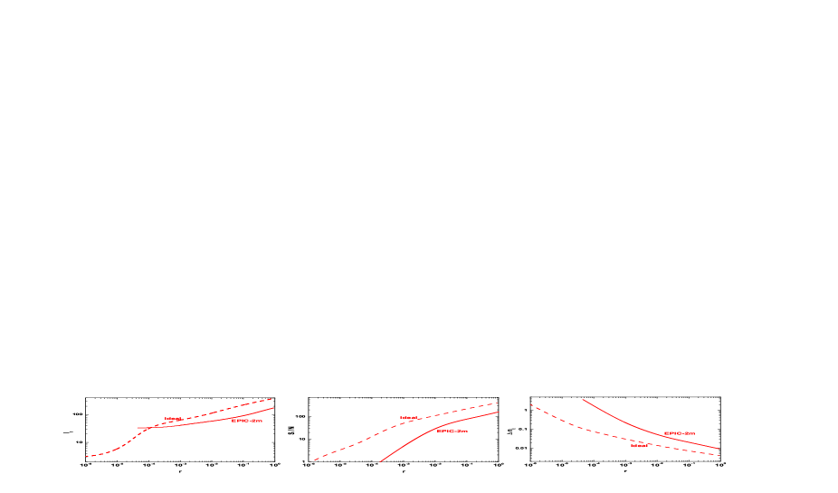
Taking into account the total noises, and using the formulae in Eqs. (9), (11), (12), we calculate the quantities , and as functions of the input tensor-to-scalar ratio . The results are shown in Fig. 1 (the red solid lines), which are consistent with the previous works zhao2011 ; ma2010 ; cmbpol . Fig. 1 shows that as expected, the model with a larger follows a larger , and a smaller . It is interesting to find that when , EPIC-2m can detect the signal of gravitational waves at more than level. For case, we have , and for , we have . So we conclude that EPIC-2m can well detect the signal of gravitational waves so long as the tensor-to-scalar ratio is larger than . At the same time, the determination of the spectral index is also quite accurate. If , one has , and if , one has . Especially, for , the uncertainty reduces to . So, it would be a quite powerful tool to study the physics in the early Universe, especially for distinguishing different inflation models, which will be shown in Sec. III.
It was noticed that the detection abilities of the future CMB experiments for the relic gravitational waves are limited by the cosmic variance and cosmic weak lensing effect (see lensingreview and references therein). Especially, when the instrumental noise power spectra of the future experiment become smaller than K2, the weak lensing contamination for the B-mode polarization could be dominant among the total noises, and forms a detection limit for the CMB experiments song2002 ; zhao2009a . A number of works have discussed methods to subtract the lensed B-mode signal (see lensing1 ; lensing2 ). In lensing2 , the authors claimed that a reduction in lensing power by a faction of , i.e. a residual faction , is possible using an approximate iterative maximum-likelihood method. For this reason, as an idealized scenario, we shall also consider the case with reduced cosmic lensing noise with . In this ideal case, we assume an exactly full sky survey with . We also assume that there are no instrumental noises or foreground emissions.
By the similar steps, we calculate the quantities , and as functions of the input tensor-to-scalar ratio in this ideal case. The results are also shown in Fig. 1 with dashed lines, consistent with zhao2009a . We find that the gravitational waves with can be detected at more than level. This can be treated as the detection limit of the CMB experiments. This lower limit corresponds to the Hubble parameter GeV, and the energy scale of inflation GeV. From Fig. 1, we also find that when , the signal-to-noise ratio becomes quite large, i.e. . In this idealized situation, the uncertainty of the spectral index also becomes very small. We can constrain to the level if , and for . Distinguishing different inflation models in this ideal case will also be presented in Sec. III.
III Testing the inflationary consistency relations
Nowadays the inflationary scenario has been widely accepted by almost all of the cosmologists. Inflation can naturally explain the well observed primordial density perturbations with a nearly scale-invariant power spectrum. However, we still do not know which inflation model describes our real Universe, since almost all the models are compatible with the current observations if the proper model parameters are adopted. So distinguishing different inflation models, especially different classes of models, is the key task for the future research.
The so-called consistency relation gives a clear difference for different classes of inflation. For example, for the cannonical single-field slow-roll inflation models, the consistency relation is held, which provides a unique way to confirm or rule out this class of models. In this section, we shall carefully investigate the possibility of testing the consistency relations for the canonical single-field slow-roll inflation, the general Lorentz-invariant single-field inflation, the phantom inflation and the potential-driven G-inflation, by the potential future observations, such as the planned CMBPol mission and the ideal CMB experiment.
III.1 Canonical single-field slow-roll inflation model
First of all, we focus on the simplest version of inflation, i.e. the canonical single-field slow-roll inflation model. In this scenario, the dynamics of Universe is governed by a scalar field (the inflaton) with canonical kinetic term. The inflaton slowly rolled down its flat potential in the inflationary stage. Inflation ended when the slow-roll conditions were broken down, and the inflaton decayed into the relativistic particles and re-heated the Universe. See some recent discussions in Alabidi:2008ej .
The Lagrangian for the canonical single-field inflation model is given by inflation
| (13) |
where is the potential of inflaton field . Different describes the different inflation models. In the inflationary stage, the potential energy of the inflaton dominates over its kinetic energy, and should be quite flat. Thus, we can define the slow-roll parameter
| (14) |
where the dot denotes , and the prime denotes . This parameter should be much smaller than one during inflation.
The tensor-to-scalar ratio and the tensor spectral index in this scenario are related to the slow-roll parameter by inflation
| (15) |
The above equations lead to the so-called consistency relation for the canonical single-field slow-roll inflation inflation (For a detailed critical discussion of this consistency relation see the last paper in grishchuk1974 ),
| (16) |
This consistency relation is independent on the form of the potential and valid for all the single-field slow-roll inflation models with canonical kinetic terms 222It was pointed out that this consistency relation could be violated if considering the trans-Planckian physics in the early Universe transplanck . So in this sense, the testing of this consistency relation also provides the change to study the trans-Planckian physics.. So testing this relation provides a model-independent criteria to confirm or rule out the canonical single-field slow-roll inflation models.
From (16), we find that testing this relation depends on the measurement of the gravitational-wave’s parameters and . Since the absolute value of is expected to be one order smaller than that of (see Eq. (16)), and the measurement of is much more difficult than zhao2009a ; zhao2009b ; ma2010 . How well we can measure the spectral index plays a crucial role in testing the consistency relation (16).
Now, let us discuss how well this consistency relation can be tested by the potential future CMB observations, which has been partly discussion in the previous works smith2006 ma2010 ; zhao2011 easson2010 . Here, we will revisit this problem based on the discussion in Sec. II, where a best-pivot wavenumber number and the best determinations of the parameters and are considered.
The uncertainty as a function of the input is replotted in Fig. 2 (red lines). We investigate if the future experiments might distinguish the tilted gravitation waves from the scale-invariant one (i.e. ). To attain the goal of this testing, in Fig. 2 we compare the value of with that of 333In principle, for any given , we should compare its value with that of , derived from the model with this as input. However, we notice that in the inflation models considered in this paper, the value of is always very close to zero, which follows that the difference between these ’s and that in Sec. II are very small. Throughout this paper, we shall ignore this little difference.. If , then the constraint on is tight enough to allow the consistency relation to be tested. We find that is satisfied only if for the EPIC-2m experiment, which is quite close to the current upper limit of obtained from the 7-year WMAP observations komatsu2010 . So we conclude that there is only a small space left for testing the consistency relation for CMBPol. This is the reason why many people claimed that the consistency relation is difficult to test cmbpol . However, from Fig. 2, we find that this situation can be slightly alleviated for the ideal observation. In this case, is satisfied so long as . Thus, it is possible to test the consistency relation (16) only for some inflation models with fairly large .
Let us consider two specific models. First, we discuss the chaotic inflation. The prototype for chaotic inflation involves a single polynomial term with liddle1983 . Here, the scale is relevant for the higher-dimensional terms in this effective potential. The chaotic inflation models of this form make the following prediction cmbpol
| (17) |
If assuming komatsu2010 and , we have . So in this model, the consistency relation could be tested by the ideal experiment. Another typical model we consider is the hill-top models with quadratic term, which has the potential form with and . This potential is considered as an approximation to a generic symmetry-breaking potential inflation ; cmbpol . If , the value of can be expressed as cmbpol
| (18) |
where is the number of e-folds, taking to be in the range based on the current observations of the CMB komatsu2010 . For , we find that . So, if this model describes our real Universe, the consistency relation cannot be tested even in the ideal case.
III.2 General Lorentz-invariant single-field inflation model
In this subsection, we will consider the general Lorentz-invariant single-field inflation model, in particular the model with non-canonical kinetic terms, such as K-inflation kinflation , Dirac-Born-Infeld (DBI) inflation alishahiha2004 , the power-law kinetic inflation seery2005 ; panotopoulos2007 and so on. These models may be motivated by the high-dimensional superstring theory or brane theory cmbpol .
The Lagrangian for general Lorentz-invariant single-field inflation takes the form
| (19) |
where . Canonical single-field inflation is included in (19). The function corresponds to the pressure of the scalar fluid, while the energy density is , where . An important parameter in this model is the speed of sound, which is defined by
| (20) |
For the canonical single-field inflation we have . However, in the general K-inflation model, the value of can be larger or smaller than speed of the light kinflation .
The parameters related to the gravitational waves can be quantified in terms of the sound speed and the slow-roll parameter kinflation , i.e.
| (21) |
Thus, the consistency relation becomes
| (22) |
When , Eq. (16) is naturally recovered. However, when or , the difference between (22) and (16) becomes obvious, and makes it possible to distinguish these two classes of models.
Due to the dependence of in the consistency relation (22), it is necessary to consider other observation to constrain the sound speed in the models. In addition to directly constrain , there are some other possibility to constrain the sound speed by the observations. For the models with , higher derivative terms in the Lagrangian are included and usually a large non-local form bispectrum is predicted. However the full bispectrum is controlled by two parameters chen2007 : and . Therefore we need two observables to fix . Fortunately, two independent templates have been well defined for measuring the non-local form bispectrum: equilateral and orthogonal forms whose sizes are respectively measured by two non-Gaussian parameters and komatsu2000 ; Babich2004 ; Senatore2009 ; komatsu2010 . In some specific cases, such as the DBI inflations alishahiha2004 and power-law kinetic inflations seery2005 ; panotopoulos2007 , and can be determined by the unique parameter . However, for the general Lorentz-invariant single-field inflations, in other2 one of us (QGH) found that the speed of sound can be fixed once both and are detected, i.e.
| (23) |
The constraints on the non-Gaussian parameters by the current and potential future CMB observations have been discussed by a number of authors komatsu2000 ; komatsu2010 ; zaldarriaga2004 ; yadav2007 ; smith2009a . Different from the constraint on the relic gravitational waves, the detection of non-Gaussian signal mainly depends on the observations of CMB , and power spectra. So, we expect that there is no degeneration between constraints of the non-Gaussian parameters and those of the gravitational-wave’s parameters. The current 7-year WMAP data indicate a constraint on the non-Gaussian parameters as follows komatsu2010 ,
| (24) |
These constraints have been obtained using the temperature signal only. The upcoming Planck satellite will improve this to the level , mainly by the observations of the E-mode polarization signal. In addition, a satellite mission such as CMBPol, dedicated to polarization and cosmic variance limited up to , would be able to further improve on Planck by a factor of order 1.6, reaching cmbpol ; komatsu . This can also be treated as the detection ability of the ideal CMB experiment, due to the cosmic variance limit.
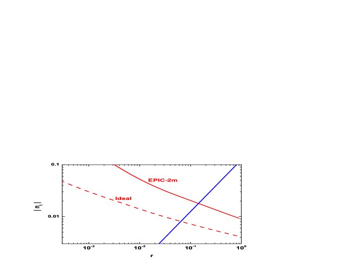
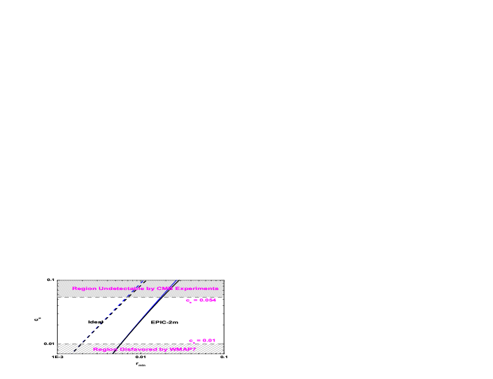
In the limit of and , signal of non-Gaussianity will be quite well observed by the future observations, such as Planck satellite planck . In this limit, we have and the consistency relation becomes . In Fig. 3, we compare values of (blue solid line) with . We find that is satisfied if for EPIC-2m experiment, and for the ideal experiment. Comparing with the conclusion in Sec.III.1, the quite promising results are expected for the study of inflation.

However, we have to mention that this is a too optimistic case. Actually, the values of could be much smaller. With the decreasing of , the value of increases, and the testing of consistency relation becomes more and more difficult. A non-Gaussian signal exceeding will be detectable from the future CMB observations cmbpol . So as another limit case, let us assume , which follows that and the consistency relation . From Fig. 3, we find that is satisfied if for EPIC-2m experiment, and for the ideal experiment. We mention that when or , the detection of non-Gaussian signal becomes impossible, and testing of the consistency relation by this method becomes impossible as well. In Fig. 4, we plot the value of (where is satisfied) for different values of in blue lines. In this figure, we use the dashed grey lines to label two limit cases considered above. It is important to mention that these results are only correct for the non-canonical Lorentz-invariant single-field inflation models. As a subclass of the general single-field inflation model, the canonical inflation model has a definite prediction . So the sound speed is not a free parameter for this subclass of models, and we do not need to constrain for the testing of the consistency relation, which has been clearly discussed in Section III.1
Recall that an important goal of inflation programs is to test whether inflation really arises from the canonical single-field slow-roll models. To attain the goal of this testing, we should compare with the quantity . If , the constraint of is tight enough to allow this test. Similar to above, for any given , we define (where is satisfied). This is the minimal , when the test is allowed. In Fig. 4, we also plot the value of for different values of in black lines. As expected, the black lines are quite close to the corresponding blue ones.
III.3 Phantom inflation model
In a spatially flat Friedmann-Lemaître-Robertson-Walker universe, the null energy condition corresponds to the inequality and hence . In order to get a blue tilted gravitational waves, one needs to break the null energy condition, for example phantom inflation piao2004 in which the Lagrangian is given by
| (25) |
The tensor-to-scalar ratio and the tensor spectral index in this scenario are related to the slow-roll parameter by
| (26) |
which leads to the consistency relation for the phantom inflation piao2004
| (27) |
This consistency relation is same as that in (16), except the sign of . Therefore the analysis on phantom inflation is exactly same as that in the canonical single-field inflation discussed in Sec. III.1. So, we can easily obtain the conclusion: is satisfied only if for the EPIC-2m experiment, for the ideal CMB experiment. However, distinguishing phantom inflation from the canonical single-field slow-roll inflation is a little easier. In order to attain this goal, we compare with . We find that is satisfied if for EPIC-2m experiment, and for the ideal experiment.
III.4 Potential-driven G-inflation model
Recently, an inflation model dubbed as “G-inflation” was proposed in g-inflation0 ; g-inflation1 ; g-inflation . In this class of models, inflation is driven by a scalar field with Galileon-like kinetic term. In g-inflation0 , the authors found that the model can generate a scale-invariant power spectrum of density perturbations, and significantly large amplitude of gravitational waves. The general Lagrangian of G-inflation is of the form
| (28) |
where and are general functions of and . If , this model returns to the general Lorentz-invariant single-field inflation discussed in Sec. III.2. In g-inflation , the potential-driven G-inflations were discussed. In this subclass of models, the Lagrangian in (28) has the following form
| (29) |
In the inflationary stage, the energy density is dominated by the potential under the slow-roll condition. In these models, the model-independent consistency relation between the tensor-to-scalar ratio and the tensor spectral index is satisfied g-inflation :
| (30) |
which is the smoking-gun evidence for the potential-driven G-inflation.
Firstly, we investigate whether it is possible to test the consistency relation in (30) by discriminating the tilted gravitational waves from the scale-invariant one. Very similar to the case with canonical single-field slow-roll inflation, we find that is satisfied if for EPIC-2m mission, and for the ideal experiment.
Another test for the consistency relation is discriminating this G-inflation from the canonical single-field inflation. To attain the goal, we compare with . Since the two consistency relations (16) and (30) are very close with each other, which induces a very small , we find that it is impossible to obtain the condition for EPIC-2m mission so long as . Even if we consider the ideal CMB observations, is satisfied only if , which is conflicted with the current constraint on komatsu2010 . So we conclude that by the CMB observations, it is impossible to discriminate the potential-driven G-inflation from the canonical single-field inflation by testing the consistency relations.
IV Conclusions
Inflationary scenario has been accepted by most cosmologists, which naturally solves the flatness, horizon and monopole puzzles in the standard hot big-bang cosmological model, and predicts the nearly scale-invariant power spectra of the primordial density perturbations and gravitational waves. Although the recent experimental efforts, including the CMB and the large-scale structure, have led to a robust detection of the primordial density perturbations, and indirectly supported the existence of the early inflationary stage, how to distinguish different inflation models still remains an outstanding experimental challenge. It depends on how accurately we can measure the primordial perturbations, in particular the primordial gravitational waves.
In this paper, based on the potential future CMB observations by the planned CMBPol mission and an ideal CMB experiment, we investigated the possible tests for the consistency relations in several classes of single-field inflation models: the canonical single-field slow-roll inflation, the general Lorentz-invariant single-field inflation, the phantom inflation and the potential-driven G-inflation. For the canonical single-field inflation, phantom inflation and the potential-driven G-inflation, we found that the consistency relations are quite hard to be tested, due to the smallness of spectral index . For example, the testing is possible only if for CMBPol mission and for the ideal experiment.
Dramatically the situation becomes quite promising for the general Lorentz-invariant single-field inflation with large non-local non-Gaussianity, because the value of could be quite large compared to that in the canonical single-field inflation for a given in these cases. For the general Lorentz-invariant single-field inflation with the non-Gaussian parameters , the testing is possible if for CMBPol mission and for the ideal experiment.
In the end of this paper, it is worthy to point out that the similar analysis can be applied to observationally test some other inflationary scenarios chain ; wands2002 . At the same time, in addition to the relations related to and , the other inflationary consistency relations (see other1 ; other2 ; other3 for instance) can also be used to distinguish different inflation models. We leave it as a future work.
Acknowledgements
We are very grateful to H.Noh, Y.S.Piao and A.Vikman for invaluable discussions. W.Z. is partially supported by NSFC Grants Nos. 11173021 and 11075141. Q.G.H. is supported by the project of Knowledge Innovation Program of Chinese Academy of Science and a NSFC Grant No. 10975167.
References
- (1) S. Weinberg, (Oxford University Press, New York, 2008).
- (2) A. H. Guth, Phys. Rev. D 23, 347 (1981); D. H. Lyth and A. Riotto, Phys. Rep. 314, 1 (1999).
- (3) Ya. B. Zeldovich, Pis’ma Astron. Zh 7, 579 (1981); L. P. Grishchuk and Ya. B. Zeldovich, in Quantum Structure of Space and Time, Eds. M. Duff and C. Isham, (Cambridge University Press, Cambridge, England, 1982), p. 409; Ya. B. Zeldovich, Cosmological field theory for observational astronomers, Sov. Sci. Rev. E Astrophys. Space Phys., Harwood Academic Publishers, Vol. 5, pp. 1-37 (1986) (http://nedwww.ipac.caltech.edu/level5/Zeldovich /Zel_contents.html); A. Vilenkin, in “The Future of Theoretical Physics and Cosmology”, Eds. G.W.Gibbons, E. P. S. Shellard and S. J. Rankin (Cambridge University Press, Cambridge, England, 2003); L. P. Grishchuk, Space Science Reviews 148, 315 (2009) [arXiv:0903.4395].
- (4) L. P. Grishchuk, Sov. Phys. JETP 40, 409 (1975); Ann. N. Y. Acad. Sci. 302, 439 (1977); JETP Lett. 23, 293 (1976) (http://www.jetpletters.ac.ru/ps/1801/article_27514.pdf); Sov. Phys. Usp. 20, 319 (1977); in General Relativity and John Archibald Wheeler, Eds. I. Ciufolini and R. Matzner, (Springer, New York, 2010) pp. 151-199 [arXiv:0707.3319].
- (5) V. F. Mukhanov, H. A. Feldman, and R. H. Brandenberger, Phys. Rep. 215, 203 (1992).
- (6) L. P. Grishchuk, Lecture Notes in Physics 562, 167 (2001); Y. Zhang, Y. F. Yuan, W. Zhao and Y. T. Chen, Classical Quantum Gravity 22, 1383 (2005); Y. Watanabe and E. Komatst, Phys. Rev. D 73, 123515 (2006); W. Zhao and Y. Zhang, Phys. Rev. D 74, 043503 (2006); L. A. Boyle and P. J. Steinhardt, Phys. Rev. D 77, 063504 (2008); M. Giovannini, Classical Quantum Gravity 26, 045004 (2009); M. L. Tong and Y. Zhang, Phys. Rev. D 80, 084022 (2009).
- (7) L. Knox, Phys. Rev. D 60, 103516 (1999).
- (8) H. V. Peiris et al., Astrophys. J. Suppl. Ser. 148, 213 (2003).
- (9) S. Chongchitnan and G. Efstathiou, Phys. Rev. D 73, 083511 (2006).
- (10) L. Verde, H. Peris and R. Jimenez, JCAP 0601, 019 (2006).
- (11) D. Baumann et al., AIP Conf. Proc. 1141 10 (2009).
- (12) M. J. Mortonson, H. V. Peiris and R. Easther, Phys. Rev. D 83, 043505 (2011).
- (13) D. A. Easson and B. Powell, arXiv:1009.3741; D. A. Easson and B. Powell, Phys. Rev. D 83, 043502 (2011).
- (14) A. Polnarev, Sov. Astron. 29, 607 (1985); L. P. Grishchuk, Phys. Rev. Lett. 70, 2371 (1993); U. Seljak and M. Zaldarriaga, Phys. Rev. Lett. 78, 2054 (1997); M. Kamionkowski, A. Kosowsky and A. Stebbins, Phys. Rev. Lett. 78, 2058 (1997); J. R. Printchard and M. Kamionkowski, Ann. Phys. (N.Y.) 318, 2 (2005); W. Zhao and Y. Zhang, Phys. Rev. D 74, 083006 (2006); D. Baskaran, L. P. Grishchuk and A. G. Polnarev, Phys. Rev. D 74, 083008 (2006); T. Y. Xia and Y. Zhang, Phys. Rev. D 79 083002 (2009).
- (15) E. Komatsu et al., Astrophys. J. Suppl. Ser. 192, 18 (2011).
- (16) W. Zhao, D. Baskaran and L. P. Grishchuk, Phys. Rev. D 79, 023002 (2009); Phys. Rev. D 80, 083005 (2009); Phys. Rev. D 82, 043003 (2010); W. Zhao, Phys. Rev. D 79, 063003 (2009); W. Zhao and L. P. Grishchuk, Phys. Rev. D 82, 123008 (2010).
- (17) P. Ade et al. (QUaD Collaboration), Astrophys. J. 674, 22 (2008); C. Pryke et al. (QUaD Collaboration), Astrophys. J. 692, 1247 (2009); S. Gupta et al. (QUaD Collaboration), Astrophys. J. 716, 1040 (2010).
- (18) H. C. Chiang et al., Astrophys. J. 711, 1123 (2010).
- (19) C. Bischoff et al. (QUIET Collaboration), arXiv:1012.3191.
- (20) C. E. North et al., arXiv:0805.3690.
- (21) http://bolo.berkeley.edu/POLARBEAR/index.html.
- (22) D. Samtleben, arXiv:0802.2657; http://quiet.uchicago.edu/.
- (23) J. A. Rubino-Martin et al., arXiv:0810.3141; http://www.iac.es/project/cmb/quijote/.
- (24) http://pole.uchicago.edu/.
- (25) http://wwwphy.princeton.edu/act/.
- (26) J. Kaplan, arXiv:0910.0391; E. Battistelli et al. (QUBIC Collaboration), arXiv:1010.0645.
- (27) http://groups.physics.umn.edu/cosmology/ebex/index.html.
- (28) A. Kogut, et al., New Astron. Rev. 50, 1009 (2006).
- (29) B. P. Crill, et al., arXiv:0807.1548.
- (30) J. Bock et al., astro-ph/0604101.
- (31) Planck Collaboration, astro-ph/0604069.
- (32) B-Pol Collaboration, Exper. Astron. 23, 5 (2009); http://www.b-pol.org/index.php.
- (33) http://cmbpol.kek.jp/litebird/.
- (34) COrE Collaboration, arXiv:1102.2181; http://www.core-mission.org/.
- (35) W. Zhao and D. Baskaran, Phys. Rev. D 79, 083003 (2009).
- (36) W. Zhao and W. Zhang, Phys. Lett. B 677, 16 (2009).
- (37) Y. Z. Ma, W. Zhao and M. L. Brown, JCAP 1010, 007 (2010).
- (38) W. Zhao, JCAP 1103, 007 (2011).
- (39) L. P. Grishchuk and M. Solokhin, Phys. Rev. D 43, 2566 (1991).
- (40) A. Kosowsky and M. S. Turner, Phys. Rev. D 52, 1739 (1995).
- (41) A. Lewis and S. L. Bridle, Phys. Rev. D 66, 103511 (2002).
- (42) G. Efstathiou and S. Gratton, JCAP 0906, 011 (2009).
- (43) J. Bock et al. (EPIC Collaboration), arXiv:0805.4207; J. Bock et al. (EPIC Collaboration), arXiv:0906.1188.
- (44) http://camb.info/.
- (45) A. Lewis, Phys. Rev. D 68, 083509 (2003); A. Lewis, A. Challinor and N. Turok, Phys. Rev. D 65, 023505 (2001); E. F. Bunn, M. Zaldarriaga, M. Tegmark and A. de Oliveira-Costa, Phys. Rev. D 67, 023501 (2003); K. M. Smith, Phys. Rev. D 74, 083002 (2006); K. M. Smith and M. Zaldarriaga, Phys. Rev. D 76, 043001 (2007); W. Zhao and D. Baskaran, Phys. Rev. D 82, 023001 (2010); J. Kim and P. Naselsky, Astron. Astrophys. 519, A104 (2010); J. Kim, arXiv:1010.2636; E. F. Bunn, arXiv:1008.0827; J. Bowyer, A. H. Jaffe and D. I. Novikov, ãrXiv:1101.0520.
- (46) A. Lewis and A. Challinor, Phys. Rep. 429, 1 (2006).
- (47) L. Knox and Y. S. Song, Phys. Rev. Lett. 89, 011303 (2002); M. Kesden, A. Cooray and M. Kamionkowski, Phys. Rev. Lett. 89, 011304 (2002).
- (48) W. Hu and T. Okamoto, Astrophys. J. 574, 566 (2002); T. Okamoto and W. Hu, Phys. Rev. D 67, 083002 (2003).
- (49) C. M. Hirata and U. Seljak, Phys. Rev. D 68, 083002 (2003); U. Seljak and C. M. Hirata, Phys. Rev. D 69, 043005 (2004).
- (50) L. Alabidi and J. E. Lidsey, Phys. Rev. D 78, 103519 (2008);L. Alabidi and I. Huston, JCAP 1008, 037 (2010);Y. Z. Ma and X. Zhang, JCAP 0903, 006 (2009).
- (51) A. Ashoorioon, J. L. Hovdebo and R. B. Mann, Nuclear Physics B 727, 63 (2005).
- (52) Y. S. Song and L. Knox, Phys. Rev. D 68, 043518 (2003); T. L. Smith, H. V. Peiris and A. Cooray, Phys. Rev. D 73, 123503 (2006).
- (53) A. D. Linde, Phys. Lett. B 129, 177 (1983).
- (54) C. Armendariz-Picon, T. Damour and V. F. Mukhanov, Phys. Lett. B 458, 209 (1999); J. Garriga and V. F. Mukhanov, Phys. Lett. B 458, 219 (1999); E. Babichev, V. Mukhanov and A. Vikman, Journal of High Energy Physics 0802, 101 (2008); V. Mukhanov and A. Vikman, JCAP 0602, 004 (2006).
- (55) M. Alishahiha, E. Silverstein and D. Tong, Phys. Rev. D 70, 123505 (2004); E. Silverstein and D. Tong, Phys. Rev. D 70, 103505 (2004).
- (56) D. Seery and J. E. Lidsey, JCAP 0506, 003 (2005).
- (57) G. Panotopoulos, Phys. Rev. D 76, 127302 (2007).
- (58) X. Chen, M. X. Huang, S. Kachru and G. Shiu, JCAP 0701, 002 (2007).
- (59) E. Komatsu and D. N. Spergel, Phys. Rev. D 63, 063002 (2001).
- (60) D. Babich, P. Creminelli and M. Zaldarriaga, JCAP 0408, 009 (2004).
- (61) L. Senatore, K. M. Smith and M. Zaldarriaga, JCAP 1001, 028 (2010).
- (62) Q. G. Huang, JCAP 1005, 016 (2010).
- (63) D. Babich and M. Zaldarriaga, Phys. Rev. D 70, 083005 (2004).
- (64) A. P. S. Yadav, E. Komatsu and B. D. Wandelt, Astrophys. J. 664, 680 (2007).
- (65) K. M. Smith, L. Senatore and M. Zaldarriaga, JCAP 0909, 006 (2009).
- (66) E. Komatsu, private communication.
- (67) Y. S. Piao and Y. Z. Zhang, Phys. Rev. D 70, 063513 (2004).
- (68) T. Kobayashi, M. Yamaguchi and J. Yokoyama, Phys. Rev. Lett. 105, 231302 (2010).
- (69) S. Mizuno and K. Koyama, Phys. Rev. D 82, 103518 (2010); C. Burrage, C. de Rham, D. Seery and A. J. Tolley, JCAP 1101, 014 (2011); P. Creminelli, G. DAmico, M. Musso, J. Norena and E. Trincherini, JCAP 1102, 006 (2011); S. Renaux-Petel, arXiv:1105.6366; S. Renaux-Petel, arXiv:1107.5020; S. Renaux-Petel, S. Mizuno and K. Koyama, arXiv:1108.0305.
- (70) K. Kamada, T. Kobayashi, M. Yamaguchi and J. Yokoyama, Phys. Rev. D 83, 083515 (2011).
- (71) A. Ashoorioon, JCAP 1004, 002 (2010).
- (72) D. Wands, N. Bartolo, S. Matarrese and A. Riotto, Phys. Rev. D 66, 043520 (2002);
- (73) P. Creminelli and M. Zaldarriaga, JCAP 0401, 006 (2004).
- (74) C. Cheung, A. L. Fitzpatrick, J. Kaplan and L. Senatore, JCAP 0802, 021 (2008).