Understanding the physics of the X-factor

Abstract

We study the relationship between the H₂ and CO abundances in simulated molecular clouds using a fully dynamical model of magnetized turbulence coupled to a detailed chemical network. We find that the CO-to-H₂ conversion factor for a given molecular cloud, the so-called X-factor, is determined primarily by the mean extinction of the cloud, rather than by its metallicity. Our results explain the discrepancy observed in low metallicity systems between cloud masses derived from CO observations and other techniques such as infrared emission, and predict that CO-bright clouds in low metallicity systems should be systematically larger and/or denser than Milky Way clouds.

1 Introduction

Observed star formation takes place within giant molecular clouds (GMCs), so understanding how these clouds form and evolve is a key step towards understanding star formation. The main chemical constituent of any GMC is molecular hydrogen (H₂), but this is very difficult to observe in situ. For this reason it is common to use emission from carbon monoxide (CO) as a proxy for H₂.

In order to do this, however, it is necessary to understand the relationship between the distributions of the H₂ and the CO. They have rather different formation mechanisms: H₂ forms on the surface of dust grains, while CO forms in the gas-phase as a product of ion-neutral chemistry. Both are readily photodissociated by ultraviolet (UV) radiation, but H₂ can protect itself from this radiation via self-shielding even in relatively low column density gas (Draine & Bertoldi [1996]). We therefore expect to find large variations in the CO/H₂ ratio within any given GMC, with the H₂ filling a significantly larger volume of the cloud than the CO.

Despite this, there is good evidence that CO emission is a good tracer of H₂ mass within the Milky Way (see e.g. Solomon et al. [1987], Dame et al. [2001]). A number of independent studies have shown that GMCs in the Galactic disk show a good correlation between the integrated intensity of the $J=1\rightarrow 0$ rotational transition line of ¹²CO and the H₂ column density. This correlation is typically described in terms of a conversion factor $X_{\rm CO}$ (the ‘X-factor’), given by

$$X_{\rm CO}=\frac{N_{\rm H_{2}}}{W_{\rm CO}}\simeq 2\times 10^{20}{\rm cm^{-2}\>K^{-1}\>km^{-1}\>s},$$ (1)

where $W_{\rm CO}$ is the velocity-integrated intensity of the CO $J=1\rightarrow 0$ emission line, averaged over the projected area of the GMC, and $N_{\rm H_{2}}$ is the mean H₂ column density of the GMC, averaged over the same area.

However, the issue of the environmental dependence of $X_{\rm CO}$ remains highly contentious. Extragalactic measurements of $X_{\rm CO}$ that use a virial analysis to determine cloud masses find values for $X_{\rm CO}$ that are similar to those obtained in the Milky Way, with at most a weak metallicity dependence (e.g. Rosolowsky et al. [2003], Bolatto et al. [2008]). On the other hand, measurements that constrain GMC masses using techniques that do not depend on CO emission consistently find values for $X_{\rm CO}$ that are much larger than the Galactic value and that are suggestive of a strong metallicity dependence (e.g. Israel [1997], Leroy et al. [2009]).

Numerical simulations provide us with one way to address this observational dichotomy. If we can understand the distribution of CO and H₂ in realistic models of GMCs, then we may begin to understand why the different types of observation give such different results. In this contribution, we summarize the results from some of our recent numerical simulations that self-consistently model both the chemistry and the turbulent dynamics of the gas within GMCs, and discuss what they can tell us about the behaviour of $X_{\rm CO}$.

2 Method

We have performed a large number of simulations of the chemical and thermal evolution of the turbulent, dense interstellar medium using a modified version of the ZEUS-MP magnetohydrodynamical code. Our modifications include the addition of a simplified treatment of hydrogen, carbon and oxygen chemistry, a detailed atomic and molecular cooling function, and a treatment of the effects of ultraviolet radiation using a six-ray approximation. Full details of these modifications can be found in Glover et al. ([2010]).

Our simulations begin with initially uniform atomic gas, threaded by a uniform magnetic field with strength $B_{0}=5.85\mbox{ }\mu{\rm G}$. The initial velocity field is turbulent, with power concentrated on large scales, and with an initial rms velocity of 5 ${\rm km}\>{\rm s^{-1}}$. We drive the turbulence so as to maintain approximately the same rms velocity throughout the simulation. We adopt periodic boundary conditions for the gas and in most cases use a cubical simulation volume with a side length $L=20$ pc. In a few simulations, we adopt a smaller-sized box, with $L=5$ pc. We have run simulations with a variety of mean densities and metallicities, in order to span a range of different physical conditions. Full details of these simulations can be found in Glover & Mac Low ([2010]).

3 Results

Because the CO in many of our simulations is optically thick, an accurate determination of $W_{\rm CO}$ would require a full non-LTE radiative transfer calculation, a complex undertaking outside the scope of our present study. Instead, we make use of a simpler procedure to determine an estimate for the CO-to-H₂ conversion factor, denoted as $X_{\rm CO,est}$. We first select a set of independent sightlines through our simulation, one per resolution element. We next compute H₂ and CO column densities along each of these sightlines. We convert each of the CO column densities into an estimate of the optical depth of the gas in the CO $J=1\rightarrow 0$ transition, under the assumptions that (a) the CO level populations are in LTE, (b) the gas is isothermal, with a temperature equal to the CO-weighted mean temperature found in the actual simulation, and (c) the CO linewidth is uniform, and is given by $\Delta v=3\>{\rm km}\>{\rm s^{-1}}$. Given an estimate for the CO optical depth, we then compute an estimate for $W_{\rm CO}$ using the same technique as in Pineda et al. ([2008]). Finally, we average over all the sightlines to compute a mean intensity $\langle W_{\rm{}_{CO}}\rangle$ for the simulation, and do the same for the H₂ to arrive at a mean H₂ column density. $X_{\rm CO,est}$ is then simply the ratio of these two values.

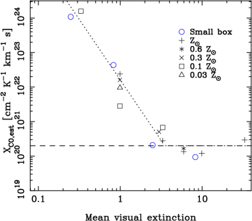
Figure 1: Estimate of the CO-to-H₂ conversion factor $X_{\rm CO,est}$, plotted as a function of the mean visual extinction of the gas, $\langle A_{\rm V}\rangle$. At $\langle A_{\rm V}\rangle>3$, the values we find are consistent with the value of $X_{\rm CO}=2\times 10^{20}{\rm cm^{-2}\>K^{-1}\>km^{-1}\>s}$ determined observationally for the Milky Way by Dame et al. ([2001]), indicated in the plot by the horizontal dashed line. At $\langle A_{\rm V}\rangle<3$, we find evidence for a strong dependence of $X_{\rm CO,est}$ on $\langle A_{\rm V}\rangle$. The empirical fit given by Equation 2 is indicated as the dotted line in the Figure, and demonstrates that at low $\langle A_{\rm V}\rangle$, the CO-to-H₂ conversion factor increases roughly as $X_{\rm CO,est}\propto A_{\rm V}^{-3.5}$.

Using this procedure, we have computed $X_{\rm CO,est}$ for each of our simulations. Figure 1 shows how the values we obtain depend on the mean visual extinction of the gas, $\langle A_{\rm V}\rangle$. We see from the figure that there is a clear change in the behaviour of $X_{\rm CO,est}$ at $\langle A_{\rm V}\rangle\sim 3$. In clouds with larger mean extinctions, $X_{\rm CO,est}$ is roughly constant and has a value consistent with the observationally-determined value for the Milky Way. On the other hand, for smaller mean extinctions, $X_{\rm CO,est}$ increases sharply with decreasing $\langle A_{\rm V}\rangle$. This behaviour is caused by a rapid fall-off in the CO abundance with decreasing mean extinction, which leads to a corresponding sharp drop in $W_{\rm CO}$. Because it does not self-shield efficiently, CO molecules are protected from photodissociation primarily by dust extinction, and so as this decreases, the CO abundance decreases much more rapidly than the H₂ abundance, resulting in the rapid increase we find for $X_{\rm CO,est}$. The dependence of $X_{\rm CO,est}$ on $\langle A_{\rm V}\rangle$ can be described by the empirical fitting function

$$X_{\rm CO,est}\simeq\left\{\begin{array}[]{lr}2.0\times 10^{20}&A_{\rm V}>3.5\\ 2.0\times 10^{20}\left(A_{\rm V}/3.5\right)^{-3.5}&A_{\rm V}<3.5\end{array}\right.$$ (2)

illustrated in Figure 1 by the dotted line.

The sharp fall-off in $W_{\rm CO}$ with decreasing mean extinction has an important consequence. In order to detect CO emission from GMCs in Local Group galaxies, the integrated intensity of the emission must be $\sim 1\,{\rm K}\,{\rm km}\,{\rm s^{-1}}$ or higher, and we find in our simulations that only the clouds with $\langle A_{\rm V}\rangle>1$ have integrated intensities above this value. Therefore, GMCs detectable in CO will always sit on the right-hand side of Figure 1, in the regime where $X_{\rm CO,est}$ is roughly constant, providing a simple explanation for why values of $X_{\rm CO}$ in extragalactic systems derived using CO observations are always roughly the same as the Galactic value. On the other hand, GMCs with mass determinations that do not rely on CO are not constrained to fall in the regime where $W_{\rm CO}$ is large, and so may occur anywhere in the plot, thereby explaining why they are often found to have X-factors that are much larger than the Galactic value. A further consequence of the behaviour of $X_{\rm CO}$ and $W_{\rm CO}$ is the prediction that CO-bright clouds in low metallicity systems must be larger and/or denser than their Milky Way counterparts, since at lower metallicity a larger surface density of gas is required to produce the necessary mean extinction.

References

- [2008] Bolatto, A. D., Leroy, A. K., Rosolowsky, E., Walter, F., & Blitz, L. 2008, ApJ, 686, 948
- [2001] Dame, T. M., Hartmann, D., and Thaddeus, P. 2001, ApJ, 547, 792
- [1996] Draine, B. T., and Bertoldi, F. 1996, ApJ, 468, 269
- [2010] Glover, S. C. O., and Mac Low, M.-M. 2010, MNRAS, in press; arXiv:1003.1340.
- [2010] Glover, S., Federrath, C., Mac Low, M.-M., and Klessen, R. S. 2010, MNRAS, 404, 2
- [1997] Israel, F. P. 1997, A&A, 328, 471
- [2009] Leroy, A. K., Bolatto, A., Bot, C., Engelbracht, C. W., Gordon, K., Israel, F. P., Rubio, M., Sandstrom, K., and Stanimirović, S. 2009, ApJ, 702, 352
- [2008] Pineda, J. E., Caselli, P., and Goodman, A. A. 2008, ApJ, 679, 481
- [2003] Rosolowsky, E., Engargiola, G., Plambeck, R., and Blitz, L. 2003, ApJ, 599, 258
- [1987] Solomon, P. M., Rivolo, A. R., Barrett, J., and Yahil, A. 1987, ApJ, 319, 730