The statistics of Wigner delay time in Anderson disordered systems

Abstract

We numerically investigate the statistical properties of Wigner delay time in Anderson disordered 1D, 2D and quantum dot (QD) systems. The distribution of proper delay time for each conducting channel is found to be universal in 2D and QD systems for all Dyson’s symmetry classes and shows a piece-wise power law behavior in the strong localized regime. Two power law behaviors were identified with asymptotical scaling ${\tau^{-1.5}}$ and ${\tau^{-2}}$, respectively that are independent of the number of conducting channels and Dyson’s symmetry class. Two power-law regimes are separated by the relevant time scale $\tau_{0}\sim h/\Delta$ where $\Delta$ is the average level spacing. It is found that the existence of necklace states is responsible for the second power-law behavior ${\tau^{-2}}$, which has an extremely small distribution probability.

I introduction

After the pioneering works,eisenbud ; wigner ; smith the problem of quantum mechanical scattering has attracted intensive research interest in many fields. The dynamical aspect of the scattering process can be characterized by the energy derivatives of the scattering matrix, known as the Wigner delay time $\tau$. Semi-classically, Wigner delay time measures the time spent by the center of a wave packet in the scattering region, which is simply related to its group velocity. Since $\tau$ is critically dependent on the transport process, it is not self-averagingavering1 ; avering2 . Hence a complete distribution is required to fully comprehend this quantity in classical chaotic or quantum disordered systems.

The distribution of delay time in 1D system has been thoroughly studied both theoretically comet ; joshi ; texier ; stein ; ossipov1 ; kumar ; amrein ; bodyfelt and experimentally.genack ; chananov Texier and Comettexier showed by various methods the universality of the distribution of $\tau$ in a 1D semi-infinite system, which has a ${\tau^{-2}}$ power-law tail at large $\tau$ in the localized regime. This power law tail has also been confirmed by others.joshi ; stein ; kumar It has been established that ${\tau^{-2}}$ behavior is valid for different types of disorder potential with $\delta$, gaussian, box, and exponential decaying distributions.comet ; joshi

For 2D systems with multichannels, most of the theoretical works are based on the random matrix theory (RMT).fyodorov1 ; seba ; brouwer ; fyodorov2 ; sommers A simple expression of $P_{N}(\tau)$ for different Dyson’s symmetry classes has been derivedseba ; fyodorov1 at the ideal coupling condition, which has a $\chi^{2}$ distribution with $\beta(N+1)$ degrees of freedom where $\beta$ is the symmetry index and N the number of conducting channels. On the other hand, a $P(\tau)\sim\tau^{-1.5}$ asymptotic behavior in the diffusive regime was numerically obtained from the kicked rotor model (KR model).ossipov2 ; kottos1 ; kottos2 Starting from RMT, it was shown that an open chaotic system weakly coupled with many open channels also exhibits the $\tau^{-1.5}$ power-law behavior in symmetry classes $\beta$=1, 2, and 4.fyodorov2 ; sommers So far all the studies are focused on diffusive regime, less attention has been paid on the localized regime. It is the purpose of this paper to fill this gap. In this paper, we wish to explore the possibility of universal behavior of the distribution of Wigner delay time $\tau$ in the localized regime.

Figure 1: sketch of the three geometries of interest. (a) 1D semi-infinite tight-binding chain; (b) 2D system; (c) QD system.

In this paper, we carry out an extensive numerical investigation of statistical properties of Wigner delay time $\tau$ in disordered systems with Anderson-type of impurities for 1D, 2D and quantum dot (QD) systems. For 1D systems, our results confirm that the distribution of Wigner delay time follows a power-law behavior ${\tau^{-2}}$ in the localized regime. For 2D and QD systems, our results show that the distribution of proper delay time of each conducting channel obeys a universal piece-wise power-law in strong localized regime that is independent of number of channels and Dyson’s symmetry index $\beta$. For a scattering system, the characteristic time scale $\tau_{0}$ is related to the group velocity $v_{g}$ of the electron, i.e., $\tau_{0}=L/v_{g}$ where $L$ is the characteristic length of the system. Our results show that when $\tau<\tau_{0}$, the distribution follows a power-law ${\tau^{-1.5}}$ while for $\tau>\tau_{0}$ a new power-law of ${\tau^{-2}}$ is obtained for the proper delay time. Our result indicates that the power-law of ${\tau^{-2}}$ can only be observed in the localized regime. The physical origin of the new power-law behavior is the existence of the so called Azbel resonant stateazbel1 ; azbel2 or necklace statenecklace1 ; necklace2 . This necklace state has a very long lifetime and is the multi-resonant state inside the scattering region in the localized regime. When the incoming electron has N conducting channels, the distribution for total delay time is given by $P(\sum_{i}\tau_{i})$. Although $P(\tau_{i})$ obeys the piece-wise power-law behavior for each proper delay time $\tau_{i}$, the distribution for total delay time behaves differently. Our results show that as $N$ increases the power-law region for ${\tau^{-1.5}}$ becomes narrow and eventually diminishes in the large N limit while the power-law region for ${\tau^{-2}}$ remains but shifts towards small $\tau$. Therefore, in the large N limit, only one power-law scaling of ${\tau^{-2}}$ survives in the localized regime. This conclusion is valid for 2D and QD systems and for three different ensembles with $\beta=1,2,4$.

This paper is organized as follows. In section II, a theoretical formalism and a numerical implementation scheme for calculating Wigner delay time are given. In section III, extensive numerical results and analysis for distribution of Wigner delay time are presented for 1D, 2D and QD systems with different symmetries ($\beta=1,2,4$). Finally a brief summary is given in section IV.

II theoretical formalism

Following Wignerwigner and Smith,smith the Wigner-Smith delay time matrix is defined in terms of the scattering matrix S as

$$Q(E)=-i\hbar S^{{\dagger}}(E)\frac{\partial S(E)}{\partial E}$$

The delay time $\tau$ is simply the summation of the diagonal elements of matrix Q(E)

$$\tau=Tr[Q]=-i\hbar Tr[S^{{\dagger}}\frac{\partial S}{\partial E}]$$ (1)

From now on we will omit the energy dependence of the relevant quantities for simplicity. Supposing there are N conducting channels, the eigenvalues of delay time matrix Q are called the proper delay times, $\tau_{1},\tau_{2},...,\tau_{N}$, which can be viewed as the contribution to the total delay time $\tau$ from the corresponding conducting channel.

Three setups under investigation are schematically illustrated in Fig.1, which are respectively (a) a 1D semi-infinite chain with length $L=1000a$ lattice points; (b) a 2D system with 80 by 80 lattice sites connected to a single lead with width $W_{0}=80a$; (c) a quantum dot system with the same number of lattice points as that of the 2D system but with a lead of narrower width $W_{0}=20a$. Here $a$ is the lattice spacing between two adjacent sites, being the length scale in the calculation. Most of numerical calculations were done using these parameters. In the present work we use the conventional nearest-neighbor tight-binding approximation and Green’s function formalism to numerically study these systems. All these geometries are connected by only one semi-infinite lead to the electron reservoir, which ensures the unitary of the scattering matrix since all electrons incident will be reflected back into the reservoir in these one-lead systems.

Assuming our 2D system is in the x-y plane. In the presence of perpendicular magnetic field and Rashba spin-orbit interaction, the generalized Hamiltonian is given by

$$H=\frac{1}{2m^{*}}[p+\frac{e\textbf{A}}{c}]^{2}+V+{\mu}B{\cdot}{\sigma}+\frac{t_{SO}}{\hbar}[\sigma\times(p+\frac{e\textbf{A}}{c})]_{z}$$ (2)

where $p$ is the momentum and $m^{*}$ the effective mass of electron. Here $V$ is the confining potential that is set to zero inside the device and infinity at the boundary of the device except at the interface of the lead. The vector potential A due to the magnetic field is expressed as A=(-By, 0, 0) under Landau gauge with B the magnetic field. $\sigma$ is the Pauli matrix and $t_{SO}$ is the strength of spin-orbit coupling. $\mu=g\mu_{B}/2$ is the magnetic moment, with $g=4$ the Lande g-factor and $\mu_{B}$ the Bohr Magneton. The tight-binding Hamiltonian with nearest-neighbor hopping has an expressionqiao

$$\begin{array}[]{cll}H=&\sum_{nm\sigma}(\varepsilon_{nm}+\epsilon_{nm})c^{\dagger}_{nm\sigma}c_{nm\sigma}\\ &-t\sum_{nm\sigma}[c^{\dagger}_{n+1,m\sigma}c_{nm\sigma}e^{-im\phi}+c^{\dagger}_{n,m-1,\sigma}c_{nm\sigma}+h.c.]\\ &-t_{SO}\sum_{nm\sigma\sigma^{{}^{\prime}}}[c^{\dagger}_{n,m+1,\sigma}(i\sigma_{x})_{\sigma\sigma^{{}^{\prime}}}c_{nm\sigma}\\ &-c^{\dagger}_{n+1,m\sigma}(i\sigma_{y})_{\sigma\sigma^{{}^{\prime}}}c_{nm\sigma^{{}^{\prime}}}e^{-im\phi}+h.c.]\end{array}$$

where $c^{\dagger}_{nm\sigma}$($c_{nm\sigma}$) is the creation (annihilation) operator for an electron on lattice site $(n,m)$. $\varepsilon_{nm}$ represents the on-site energy, with magnitude 2t for 1D chain and 4t for 2D square lattice. Here $t=\hbar^{2}/2m^{*}a^{2}$ is the nearest-neighbor hopping energy, which is the energy scale in this work. Disorder energy $\epsilon_{nm}$, which is Anderson-type with a uniform distribution in the interval [-W/2,W/2], is added to the on-site energy $\varepsilon_{nm}$ with W the disorder strength.

Based on the tight-binding Hamiltonian, the retarded Green’s function in real space is defined as

$$G^{r}(E)=(E-H-\Sigma^{r})^{-1}$$

where $\Sigma^{r}$ is the self-energy of the lead, which can be calculated by a transfer matrix methodtransfer . E is the electron Fermi energy and chosen to be at the center of the corresponding subband. By the Fisher-Lee relationfisher which connects the scattering matrix and the Green’s function, the delay time $\tau$ is rewritten in terms of $G^{r}$ as

$$\tau=-i\hbar Tr[S^{{\dagger}}\frac{\partial S}{\partial E}]=\hbar Tr[G^{r}\Gamma G^{a}]$$ (3)

where $G^{a}$ is the advanced Green’s function, $G^{a}=(G^{r})^{\dagger}$, and $\Gamma$ is the line width function describing coupling of the lead to the scattering region which is given by $\Gamma=i[\Sigma^{r}-\Sigma^{a}]$. In the presence of large disorders, the system can either be in diffusive or localized regimes depending on the dimensionless localization length $\xi/L$. In the localized regime, the localization length can be defined aslocalength $<G>=C\exp(-2L/\xi)$ with G the conductance and C is a constant to be determined. To eliminate C, the localization length $\xi$ at a particular disorder strength can be obtained from

$$\xi=\frac{2L_{2}-2L_{1}}{ln<G_{1}>-ln<G_{2}>}.$$

From Eq.(3), it is clear that the calculation of Wigner delay time is equivalent to that of density of states. In our numerical calculation, the real space Green’s function can be obtained by matrix inversion which is very time-consuming. For delay time, one only needs the first $N_{lead}$ columns of Green’s function where $N_{lead}$ is the dimension of the line width function $\Gamma$. The transfer matrix method is suitable for this purpose and is fast. To study the statistics of $\tau$, we need to generate an ensemble of different realizations of the disordered systems. As we will show in the next section, the distribution of $\tau$ has a new power-law for large delay time $\tau>\tau_{0}$. These large delay times correspond to rare events with extremely small probability, which means that to study the new power-law regime of $P(\tau)$ a large configuration ensemble is necessary. Therefore intensive computation is required to accumulate enough data for statistical analysis. To speed up the calculation, we can rewrite the line width function $\Gamma$ asjian

$$\Gamma=i[\Sigma^{r}-\Sigma^{a}]=\sum_{i}^{N}|W_{i}\rangle\langle W_{i}|$$

where N is the number of conducting channels in the lead and $|W_{i}>$ is the renormalized eigenfunction of $\Gamma$. Then the delay time can be expressed as

$$\tau=\hbar Tr[G^{r}\Gamma G^{a}]=\hbar\sum_{i}^{N}(G^{r}|W_{i}\rangle)(G^{r}|W_{i}\rangle)^{{\dagger}}$$ (4)

This representation can speed up the numerical calculation and also enables to calculate the proper delay time $\tau_{i}$ from the $i-th$ conducting channel. Our results show that using the LU decomposition with multi-frontal algorithm to solve the linear equation $(E-H-\Sigma^{r})\psi_{i}=|W_{i}>$ is faster than the transfer matrix method especially for large system size like $100\times 100$. So far we have discussed the algorithm to study the statistics of $\tau$. The numerical results and relevant discussions is the content of the next section.

III numerical results and discussion

In this section, we will present our numerical results. To test our code, we first show results of 1D systems with orthogonal symmetry, in which case the distribution of $\tau$ has been studied thoroughly. Then in the following two subsections, we shall discuss in detail the cases of 2D and QD systems with different symmetries and number of conducting channels.

III.1 1D tight-binding chain

For the 1D system, Texier and Comettexier derived an analytic expression of the distribution of Wigner delay time in the localized regime for high energies or weak disorder strengths. It was found that $P(\tau)$ has an algebraic tail in the localized regimekottos2

$$P(\tau)=\frac{\xi}{\upsilon\tau^{2}}e^{-\xi/\upsilon\tau}$$ (5)

where $\xi$ is the localization length and $\upsilon$ is the group velocity. They also found numerically that in the ballistic regime $P(\tau)$ obeys a Gaussian distribution. The disorder used in their numerical simulation is the $\delta$ potential with random position in the system.

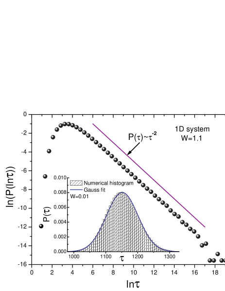
Figure 2: The distribution of Wigner delay time of a 1D semi-infinite long chain at disorder strength $W=1.1$. Inset is the normalized distribution histogram of $\tau$ at $W=0.01$. Blue curve shows the Gaussian fitting of the histogram. 4,000,000 configurations have been generated at each disorder strength W.

We have calculated the delay time distribution for a 1D tight-binding chain in both the ballistic regime and the localized regime at a relative high energy $E=1.0$ with disorder strength $W=0.01$ and $W=1.1$, respectively. The result is shown in Fig.2. Clearly the delay time distribution has a Gaussian shape at weak disorder $W=0.01$ when $L\ll\xi$ (see inset of Fig.2). As W increases, $P(\tau)$ transforms gradually from a symmetric Gaussian distribution to a one-sided distributionone-sided . To make the behavior more transparent, one may change the variable from $\tau$ to its natural logarithm. Take Eq.(5) as an example. When we use $\ln\tau$ as the variable, $P(\ln\tau)=\tau P(\tau)$, and taking logarithm at both sides, one arrives at

$$\ln P(\ln\tau)=\ln\frac{\xi}{\upsilon}-\ln\tau-\frac{\xi}{\upsilon}\frac{1}{\tau}$$ (6)

The first term in the above expression is a constant for a specific disorder strength and the last term tends to zero when $\tau$ is very large. As a result, a linear tail arises in the $\ln P(\ln(\tau))-\ln\tau$ curve. In Fig.2 we see that the linear tail of $\ln P(\ln(\tau))$ at disorder strength $W=1.1$, where the system is already localized ($L\gg\xi$), can be well fitted by a straight line with a slope $-1$, which implies that $P(\tau)\propto 1/\tau^{2}$ in the large $\tau$ region. We notice that there is a departure from the straight line at the end of the distribution curve. This departure can be improved by using more configurations, since the larger the $\tau$, the smaller its occurrence probability. We will explain the origin of these large $\tau$ in the next subsection.

To summarize briefly, our numerical results for Anderson-disordered 1D system are consistent with the conclusion of Texier and Comettexier , which confirms the universality of the $1/\tau^{2}$ power-law tail.

III.2 2D square lattice

Figure 3: Panel (a) is the distribution histogram of $\tau$ at disorder strength $W=0.0001$ and the blue curve is a standard Gaussian fitting. Panel (b) is $P(\tau)$ at $W=15$ and the corresponding histogram with variable changed to $\ln\tau$ is displayed in panel (c). Panel (d) contains the $\ln P(\ln\tau)$ versus $\ln\tau$ curves for $W=5,15,25$, and $40$. Panel (e) and (f) are respectively the asymptotic behavior of slopes for different linear sections in panel (d)’s $\ln P(\ln\tau)$ curves. The system is under such conditions: N=1 and $\beta=1$.

For 2D systems, most theoretical works of delay time distribution were within the random matrix theory. As we know, the random matrix theory works well in the diffusive regime. However, it becomes difficult to describe properties in the localized regime. In the diffusive regime, RMT predicts that $P(\tau)$ showsfyodorov2 ; sommers a universal power-law behavior $\tau^{-1.5}$, which was confirmed by a KR modelossipov2 ; kottos1 . Our numerical results for proper delay time obtained from 2D Anderson systems also show the $\tau^{-1.5}$ power-law behavior in the intermediate range of $\tau$ and reveal new properties of the distribution of Wigner delay time in the localized regime.

First we start with the simplest case of single conducting channel $N=1$ with preserved time-reversal symmetry ($\beta=1$) and the results are shown in Fig.3. Fermi energy of electron is chosen to be at the center of the first subband, $E=0.004$. From panel (a) of Fig.3 it is obvious that in the ballistic regime the distribution of Wigner delay time $\tau$ has a natural Gaussian shape at a weak disorder $W=0.0001$, which is the same as that of 1D systems. As the disorder increases, $P(\tau)$ is no longer symmetrically distributed but spreads over a wide range with a one-sided peak located at small delay time region, as shown in panel (b) with $W=15$. From the calculation of localization length $\xi$, we know that the system is localized at such a disorder strength. Therefore to get an overview of the distribution including the long delay time tail, we change the variable from $\tau$ to $\ln\tau$ and the histogram of $P(\ln\tau)$ is depicted in panel (c). Based on Eq.(6) and the argument therein, we plot the logarithm of the distribution of $\ln\tau$ in panel (d) for different disorder strengths ranging from $W=5$ to $W=40$. We see that as the disorder is increased in the scattering region, the curve of $\ln P(\ln\tau)$ vs $\ln\tau$ gradually evolves into a piece-wise power-law pattern with two different power-laws and an abrupt change from one to the other at a particular value of $\tau_{0}$. This picture becomes clear when W increases to 40. We understand this behavior as follows. In the scattering system, the characteristic time scale is set by $\tau_{0}=L/v_{g}$ with $L\sim 3L_{0}$ where $L_{0}$ is the dimension of the scattering region and $v_{g}$ is the group velocity. In the strong localized regime, there are two kinds of scattering event naturally separated by $\tau_{0}$, one corresponds to the usual direct reflection with delay time $\tau<\tau_{0}$ and the other corresponds to multi-resonant reflection with long delay time $\tau>\tau_{0}$. For Fig.3 with $L_{0}=80$, $\tau_{0}=3L_{0}/v_{g}$ gives $\ln\tau_{0}\sim 7.5$ which is close to the transition point from the power-law $\tau^{-1.5}$ to the power-law $\tau^{-2}$ in Fig.3. For strong disordered systems, the large delay time scattering events with $\tau>\tau_{0}$ are really rare events with extremely small probability. In addition, this probability decreases as W increases. For instance, the probability $P(\tau)|_{\tau>\tau_{0}}$ is $13\%$ for $W=15$ while for $W=40$ it drops to $0.32\%$. To study such rare events, more and more configurations of disordered samples are required for statistic analysis to get an accurate result. For $W=40$ we have used an ensemble of over 40,000,000 different realizations.

Another point worth noticing is that the exponents of two power-laws decrease slowly as disorder strength is increased. These two exponents versus disorder strength W are plotted in panels (e) and (f), which converge towards -0.5 and -1.0, respectively. We note that the curve in panel (f) has larger error bars compared with that in panel (e). This is understandable since large $\tau$ is more difficult to sample.

Since the computation is getting extremely time-consuming it is very difficult if not impossible to obtain the plot shown in panels (e) and (f) for large disorder strengths. Hence we decide to calculate $P(\tau)$ for a particular disorder strength which is large enough to determine the exponents for both power-law behaviors. After some trial and error, we found the disorder strength $W=100$ is appropriate for this purpose. The exponent of power-law in the intermediate region is already converged at such a W and does not change upon further increasing of disorder strength to $W=200$. To get a clear view of the tail with small probability, a large ensemble of 420,000,000 configurations is accumulated and the analyzed data is shown in Fig.4. Clearly the algebraic tail where $\tau>\tau_{0}$ is invisible in the histogram of panel (a), since it accounts for only 0.118 % in the ensemble. From panel (b) one clearly sees that the first power-law of $\ln P(\ln\tau)$ has a slope of -0.5, corresponding to a power law distribution $P(\tau)\sim\tau^{-1.5}$. After a transition region around $\tau=\tau_{0}$ shown by the blue circle in Fig.4, the second power-law distribution is found to have a slope of -1, which means that it is a power-law tail $P(\tau)\sim\tau^{-2}$. The fluctuation at the end of the tail arises because there is not enough configurations. In such a strong localized regime with $W=100$, delay time with magnitude $\ln\tau>15$ often has a few configurations out of the total 420,000,000 ensemble.

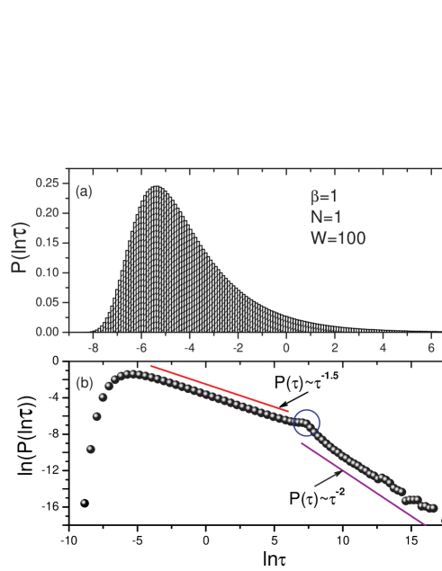
Figure 4: Statistics of Wigner delay time at disorder strength $W=100$ for $N=1$. Panel (a) is the $P(\ln\tau)$ histogram and panel (b) is the corresponding $\ln P(\ln\tau)-\ln\tau$ curve. Red and purple straight lines individually have slope -0.5 and -1.0.

The power-law distribution $\tau^{-1.5}$ has already been predicted by RMTfyodorov2 ; sommers and was also confirmed numerically using KR modelkottos2 in the diffusive regime. Our results show that this power law $\tau^{-1.5}$ for each proper delay time exists for any $N$ where $N$ is the number of conducting channels (also see numerical results presented below). In addition, this behavior persists in the strong localized regime. Importantly, the $\tau^{-2}$ algebraic tail is a novel feature that has not been reported before in 2D systems. The physical origin of the novel power-law behavior is due to the Azbel resonance states or necklace statesazbel1 ; azbel2 ; necklace1 , which are extended states in localized systems. Since in the localized regime most of the electron states are localized, these necklace states or Azbel resonances survive through multiple-resonances. These states are really rare events in the disordered samples so that they have an extremely small probability to occur. For example, in the above calculation with N=1 and $W=100$, the probability for those states with $\tau>\exp(8)$ is $0.03\%$. Despite of their rare nature, these states can play a significant role in the distribution function of delay time and dominate in the density of states in disordered systems. It is because a necklace state experiences multiple resonant scattering giving rise to a large density of states. For instance, emittance calculations in disordered 1D, 2D, and QD systems show that due to the necklace states, the average emittance remains negative in the localized regime.emittance In fact, the existence of necklace states has already been observed through optical experimentnecklace2 in a quasi-1D system. The fact that the signature of necklace states is observed again in disordered 2D systems with single lead indicates that the non-localized necklace states are generic in strong disordered systems, although difficult to see them.

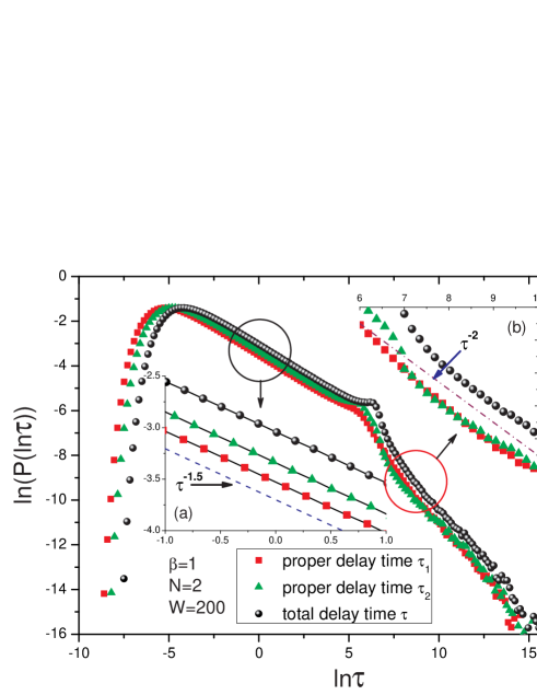
Figure 5: Distributions of proper delay time $\tau_{1}$ and $\tau_{2}$ and the total $\tau$ at disorder strength $W=100$ in the case of 2 conducting channels. Inset panel (a) highlights the first linear section of distribution with a -0.5 slope (blue-dash straight line), while panel (b) for the algebraic tail with a -1 slope (purple-dash-dot-dash straight line). Ensemble size is 150,000,000.

Next we consider the case of two conducting channels ($N=2$) in a system with $\beta=1$. Here electron Fermi energy is fixed at the center of the second subband, where $E=0.01$. Since the group velocity of electron incident from different subbands are different, proper delay times for different conducting channels are not statistically equivalent. Hence the properties of the proper delay time $\tau_{i}$, which describes the scattering of electron of the $i^{th}$ channel, as well as the total Wigner delay time $\tau={\sum_{i}}^{N}\tau_{i}$ are studied separately. To save computational time, we calculated the distribution of relevant times only at a large disorder strength $W=100$. As we have seen above, at this $W$ $P(\tau)$ of $N=1$ converges to the piece-wise power-law ($\tau^{-1.5}$ and $\tau^{-2}$) behavior. Statistically analyzed result upon an ensemble of 150,000,000 configurations is shown in Fig.5. To separate the curves we zoom in the picture around two particular areas of the two power-law regions, which are highlighted in the insets.

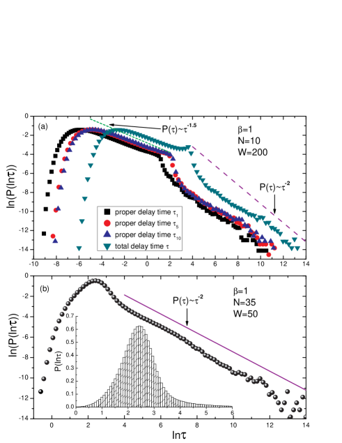
Figure 6: Panel (a) shows the distribution of proper delay time $\tau_{1}$, $\tau_{5}$, and $\tau_{10}$ as well as the total delay time $\tau$ at $W=200$ with 10 conducting channels in the lead. Panel (b) contains the normalized distribution histogram and its logarithm correspondence of total delay time $\tau$ at $W=50$ for $N=35$.

From Fig.5 it is clear that proper delay time $\tau_{1}$ and $\tau_{2}$ follow the same distribution with different constants ($P(\tau_{1/2})\sim C_{1/2}\tau^{\alpha}$ with $\alpha=$ -1.5 or -2). It shows that the proper delay time of the first and second subbands are statistically independent. Since the total delay time $\tau$ is the summation of $\tau_{1}$ and $\tau_{2}$, it is not surprising that the distribution of total delay time $\tau$ keeps the essential feature of individual proper delay time. Clearly all three curves show piece-wise power-law behaviors, which is similar to the case of a single channel $N=1$ (see Fig.4). In view of the distribution for systems with $N=1$ and $N=2$, we expect that the delay time distribution in multichannel case ($N\geq 2$) also show piece-wise power-law behavior. However the transition region in the distribution curve of $\tau$ is broadened due to the overlap of $P(\tau_{1})$ and $P(\tau_{2})$. As the channel number increases, this may lead to a significant change of the distribution form as will be discussed in detail below.

Numerical results for cases of more conducting channels $N=10$ and 35 within orthogonal ensemble ($\beta=1$) are shown in Fig.6. Following observations are in order. (1). For a strong disorder strength W=200, statistical analysis on the distribution of proper delay time at $N=10$ shows that the individual $\tau_{i}$ exhibits a piece-wise power-law behavior with two scalings $\tau^{-1.5}$ and $\tau^{-2}$, similar to that of the proper delay time in $N=2$ case. In addition, the total delay time distribution $P(\tau)$ at $N=10$ given by the superposition of all the $P(\tau_{i})$ (i=1,2,.., 10) results in the same behavior (see panel (a)). We also note that due to the group velocity difference for different subbands, the transition point $\tau_{0}=3L_{0}/v_{g}$ of proper delay time distribution is not at the same position in $\ln P(\ln\tau)$-$\ln\tau$ curve. The transition value of proper delay time is the smallest for the first subband while the largest for the highest subband. The overlap of proper delay time distribution causes the broadening of transition region of the distribution $P(\tau)$. (2). Comparing the situations of $N=2$ and $N=10$ (Fig.5 and panel (a) of Fig.6), the broadening is more obvious at large N. When the number of conducting channel increases to $N=35$, the broadening is so significant that it destroys the power-law behavior of $\tau^{-1.5}$ in the total delay time distribution although $\tau^{-1.5}$ power-law exists for each proper delay time distribution. Therefore our results suggest that in the large N limit, only the power-law of $\tau^{-2}$ survives.

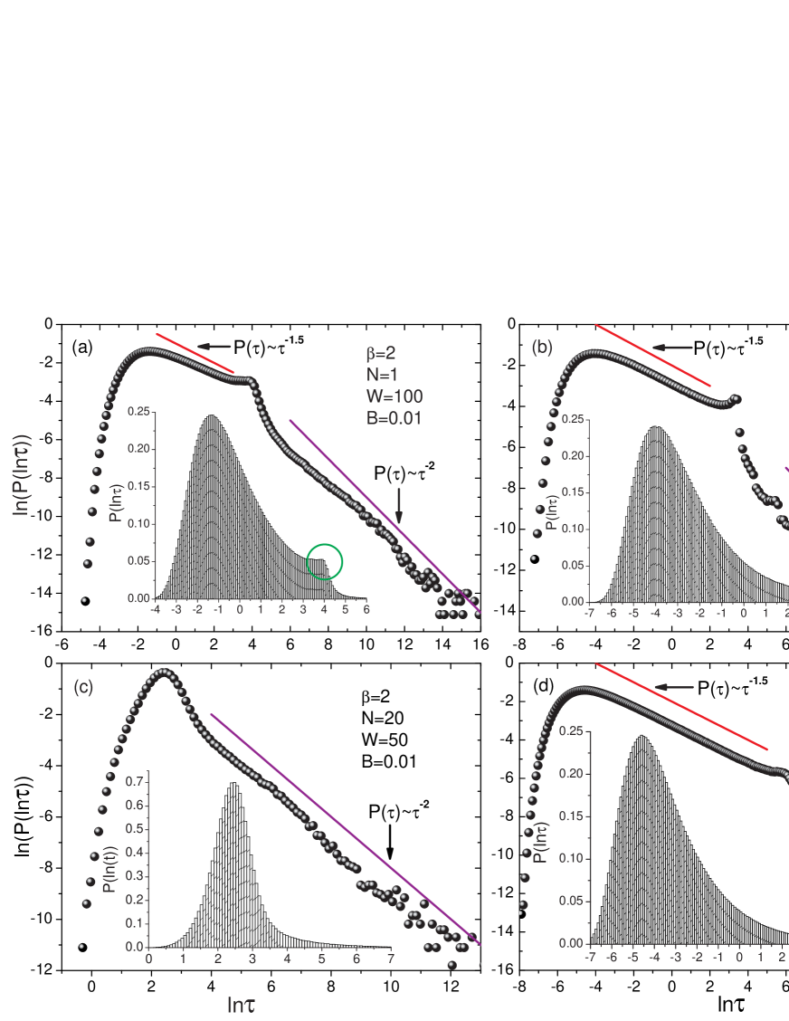
Figure 7: Panel (a) and (b) are respectively the distributions of delay time at two different sets of parameter. In panel (a) it is $W=100$ and $B=0.01$, while in (b) $W=400$ and $B=0.02$. Both systems have single conducting channel($N=1$) in unitary symmetry case ($\beta=2$). Ensemble size is 63,000,000. Panel (c) shows the statistics of $\tau$ at multi-channel case with $N=20$ at $\beta=2$. Case of symplectic symmetry case ($\beta=4$) is drawn in panel (d) with $W=100$and $N=1$, where an ensemble of size 120,000,000 configurations is used.

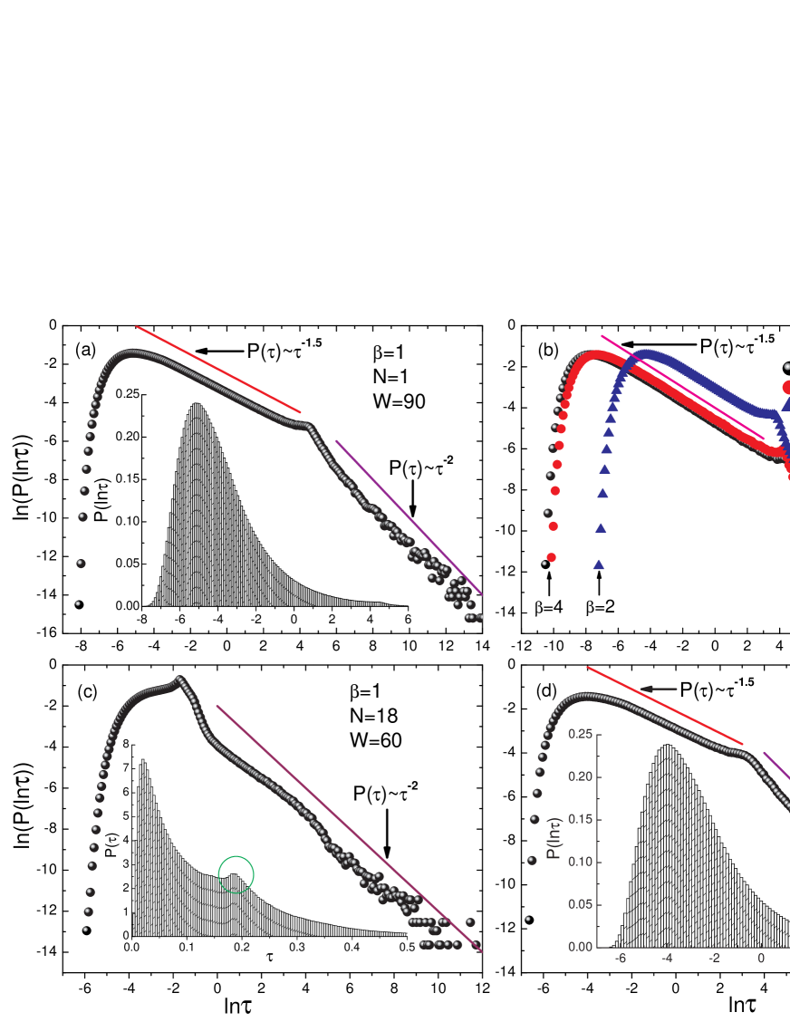
Figure 8: Quantum dot case. Panel (a) and (b) are the distribution of delay time for different symmetry classes ($\beta=1,2$, and 4) with single conducting channel($N=1$). Panel (c) corresponds to $N=18$ in orthogonal symmetry $\beta=1$. Calculation parameters are shown in the graphs. The result of a large QD at $\beta$=1 is presented in panel (d).

Now we turn to the systems with symmetry class $\beta=2$ where the time reversal symmetry is broken and $\beta=4$ in the absence of spin-rotation symmetry. In our numerical calculation, the unitary symmetry class ($\beta=2$) is realized by applying an external magnetic field while for symplectic symmetry ($\beta=4$) we consider the spin-orbit interaction. In both unitary and symplectic cases we mainly numerically investigate the statistics of Wigner delay time for single conducting channel ($N=1$) since the computation is getting extremely time-consuming for 2D with $\beta=2$ and 4. From the discussion in orthogonal symmetry case, some intuition can be obtained for the distributions of delay time at multi-channel case. From Fig.7 we see that there are clearly two power-law regions with exponents approaching $-1.5$ and $-2$ for total delay time distribution when N=1 (panels (a) and (b)). We have tested two different magnetic field strengths and they give similar results. In addition, the transition phenomena from one power-law to another can also be seen from inset of Fig.7(a) and (b) that are different from the case with $\beta=1$. We have checked that the proper delay time distribution follows a piece-wise power-law behavior. From our experience in orthogonal ensemble we expect that the $\tau^{-1.5}$ intermediate region will be destroyed at large N. Indeed, our results confirm this expectation (see panel (c) where $N=20$ is investigated). Except for this difference shown by green circles in Fig.7, the delay time distribution is similar to that of the system with reserved time-reversal symmetry ($\beta=1$)(panel (a) of Fig.4). Finally, in the case of symplectic symmetry, the distribution is the similar to that of $\beta$=1. We have also varied the strength of spin-orbit coupling $t_{SO}$ and found that it does not affect the distribution behavior.

To briefly summarize our results for 2D systems, the Wigner delay time distribution in the 2D lattice system shows a piece-wise power-law feature in strong localized regime, with power-law converging to $\tau^{-1.5}$ in the intermediate region and the algebraic tail obeying a different power law $\tau^{-2}$ for a single conducting channel. The two power-law regions are separated by a clear transition region determined by $\tau_{0}$ in the distribution curve. For multi-conducting channels, the distribution of each proper delay time is found to have the same power-law distribution as that of the delay time $\tau$ for $N=1$. For a few conducting channels, the distribution of total Wigner delay time behaves like that of a single channel. When N is large, however, the superposition of each proper delay time distribution gives rise to a broad transition region that gradually destroys the $\tau^{-1.5}$ power-law region. In the large N limit, only one power-law region exists which corresponds to $\tau^{-2}$. These features seem to be independent of symmetry class of 2D systems, i.e., regardless of orthogonal, unitary or symplectic symmetries.

III.3 Quantum dot system

The quantum dot (QD) system consists of a square scattering region and single lead attached at the right side with 1/4 width of the scattering region, as shown in Fig.1. Numerical results depicted in Fig.8 show that the conclusions obtained in 2D system are also applicable to QD case. In Fig.8(a) and (b), we see that the piece-wise power-law behavior is observed again in all Dyson’s symmetry classes for the case of $N=1$. For $\beta=1$ and $N=18$, we see that the power-law $\tau^{-1.5}$ no longer exists that is similar to the situation in 2D systems. A slight difference compared to the 2D case is that there is an additional peak in the distribution of delay time $P(\tau)$ vs $\tau$ that indicates the onset of the power-law region of $\tau^{-2}$(see panel (c) of Fig.8). To check the size effect of the distribution, we have examined a larger quantum dot system with size of $L=100$ and lead width $W_{0}=10$. The numerical results for $\beta=1$ and $N=1$ are shown in Fig.8(d) and similar conclusion can be drawn.

IV conclusion

In conclusion, we numerically investigate the statistical properties of Wigner delay time in Anderson disordered 1D, 2D and quantum dot systems for different symmetry classes $\beta=1,2,4$. The proper delay time distribution is found to be universal in strong localized regime for 2D and QD systems and shows a piece-wise power-law behavior. In addition to the known power-law scaling region ${\tau^{-1.5}}$, a novel power-law region of ${\tau^{-2}}$ is identified in the localized regime, which is independent of the number of conducting channel N and Dyson’s symmetry classes $\beta$. Our results indicate that the existence of necklace states is responsible for the $\tau^{-2}$ algebraic tail, which are rare events and have an extremely small distribution probability. The total delay time distribution can behave differently. For a few conducting channel, there is a crossover region from one power-law region to another. As the number of conducting channels N increases, this crossover region broadens and the power-law region of ${\tau^{-1.5}}$ becomes narrow. In the large N limit, the power-law of ${\tau^{-1.5}}$ is destroyed due to the broadening of the crossover region and only the $\tau^{-2}$ algebraic tail survives.

V acknowledgments

This work is supported by RGC grant (HKU 705409P) from the HKSAR and LuXin Energy Group. We thank the HPC POWER of the computer center, HKU for computation resources allocation.

References

- (1) L. Eisenbud, Ph. D dissertation, Princeton University, 1948.
- (2) E. P. Wigner, Phys. Rev. 98, 145 (1955).
- (3) F. T. Smith, Phys. Rev. 118, 349 (1960).
- (4) A. Z. Genack, P. Sebbah, M. Stoytchev, and B. A. van Tiggelen, Phys. Rev. Lett. 82, 715 (1999).
- (5) B. A. van Tiggelen, P. Sebbah, M. Stoytchev, and A. Z. Genack, Phys. Rev. E. 59, 7166 (1999).
- (6) Z. Qiao, Y. Xing, and J. Wang, Phys. Rev. B. 81, 085114 (2010).
- (7) M. P. López Sancho, J. M. López Sancho and J. Rubio, J. Phys. F: Met. Phys. 14, 1205 (1984); M. P. López Sancho, J. M. López Sancho and J. Rubio, J. Phys. F: Met. Phys. 15, 851 (1985).
- (8) D. S. Fisher, and P. A. Lee, Phys. Rev. B 23, 6851 (1981).
- (9) A. MacKinnon and B. Kramer, Phys. Rev. L 47, 1546 (1981); A. MacKinnon and B. Kramer, Z. Phys. B: Condens. Matter 53, 1 (1983).
- (10) J. Wang, and H. Guo, Phys. Rev. B 79, 045119 (2009).
- (11) A. Comet and C. Texier, J. Phys. A 30, 8017 (1997).
- (12) S. K. Joshi, A. K. Gupta and A. M. Jayannavar, Phys. Rev. B 58, 1092 (1998).
- (13) C. Texier and A. Comet, Phys. Rev. Lett. 82, 4220 (1999).
- (14) F. Steinbach, A. Ossipov, T. Kottos, and T. Geisel, Phys. Rev. Lett. 85, 4426 (1999).
- (15) A. Ossipov, T. Kottos and T. Geisel, Phys. Rev. B 61, 11411(2000).
- (16) S. A. Ramakrishna and N. Kumar, Eur. Phys. J. B 23, 515(2001).
- (17) W. O. Amrein, and Ph. Jacquet, Phys. Rev. A 75, 022106(2007).
- (18) J. D. Bodyfelt, J. A. Méndez-Bermúdez, A. Chabanov and T. Kottos, Phys. Rev. B 77, 045103(2008).
- (19) A. Z. Genack, P. Sebbah, M. Stoytchev, and B. A. van Tiggelen, Phys. Rev. Lett. 82, 715 (1999).
- (20) A. A. Chabanov and A. Z. Genack, Rev. Lett. 87, 233903 (2001).
- (21) K. A. Muttalib and P. Wolfle, Phys. Rev. Lett. 83, 3013 (1999).
- (22) Y. V. Fyodorov and H.-J. Sommers, Phys. Rev. Lett 76, 4709 (1996).
- (23) P. Sěba, K. Życzkowski and J. Zakrzewski, Phys. Rev. E 54, 2438 (1996).
- (24) P. W. Brouwer, K. M. Frahm, and C. W. J. Beenakker, Phys. Rev. Lett 78, 4737 (1997).
- (25) Y. V. Fyodorov, D. V. Savin and H.-J. Sommers, Phys. Rev. E 55, R4857 (1997).
- (26) H.-J. Sommers, D. V. Savin, and V. V. Sokolov, Phys. Rev. Lett 87, 094101 (2001).
- (27) A. Ossipov, T. Kottos and T. Geisel, Europhys. Lett 62, 719(2003).
- (28) T. Kottos, A. Ossipov and T. Geisel, Phys. Rev. B 68, 066215(2003).
- (29) T. Kottos, J. Phys. A: Math. Gen. 38, 10761(2005).
- (30) A. D. Mirlin, Physics Reports 326, 259 (2000)
- (31) M. Y. Azbel, Phys. Rev. B 27, 3852 (1983); M. Y. Azbel, Phys. Rev. B 28, 4106 (1983).
- (32) C. Basu, A. Mookerjee, A. K. Sen, and A. K. Thakur, J. Phys.: Condens. Matter 3, 9055 (1991).
- (33) J. B. Pendry, J. Phys. C: Solid State Phys. 20, 733 (1987).
- (34) J. Bertolotti, S. Gottardo, and D. S. Wiersma, Phys. Rev. Lett 94, 113903 (2005).
- (35) W. Ren, F. M. Xu, and, J. Wang, Nanotechnology 19, 435402 (2008).
- (36) C. W. J. Beenakker, Rev. Mod. Phys 69, 731 (1997).