Abstract – Convex support, the mean values of a set of random variables, is central in information theory and statistics. Equally central in quantum information theory are mean values of a set of observables in a finite-dimensional C*-algebra ${\mathcal{A}}$, which we call (quantum) convex support. The convex support can be viewed as a projection of the state space of ${\mathcal{A}}$ and it is a projection of a spectrahedron.

Spectrahedra are increasingly investigated at least since the 1990’s boom in semidefinite programming. We recall the geometry of the positive semi-definite cone and of the state space. We write a convex duality for general self-dual convex cones. This restricts to projections of state spaces and connects them to results on spectrahedra.

Our main result is an analysis of the face lattice of convex support by mapping this lattice to a lattice of orthogonal projections, using natural isomorphisms. The result encodes the face lattice of the convex support into a set of projections in ${\mathcal{A}}$ and enables the integration of convex geometry with matrix calculus or algebraic techniques.
Index Terms – state space, spectrahedron, mean value, convex support, duality, face lattice, projection lattice, poonem.
AMS Subject Classification: Primary 81P16, 62B10, 52A20 Secondary 94A17, 90C22, 90C30.

1 Quantum information, optimization & geometry

Quantum information theory is based on C*-algebras, see e.g. Amari and Nagaoka, Bengtsson and Życzkowski, Holevo, Nielsen and Chuang or Petz [AN, BZ, Ho, NC, Pe] for statistical issues or Murphy, Davidson or Alfsen and Shultz [Mu, Da, AS] about operator algebras. If ${\mathcal{A}}$ is a finite-dimensional C*-algebra we denote its dual space of linear functionals by ${\mathcal{A}}^{*}$. A state on ${\mathcal{A}}$ is a functional $f\in{\mathcal{A}}^{*}$ such that for all $a\in{\mathcal{A}}$ we have $f(a^{*}a)\geq 0$ and for the multiplicative identity ${\rm 1\mskip-4.0mul}$ of ${\mathcal{A}}$ we have $f({\rm 1\mskip-4.0mul})=1$. The set of states is the state space. This is a convex body, i.e. a compact and convex set. We denote the real vector space of self-adjoint operators by ${\mathcal{A}}_{\rm sa}$, self-adjoint operators are also called observables. The abelian algebra ${\mathcal{A}}\cong{\mathbb{C}}^{n}$, $n\in{\mathbb{N}}$, is a model of probability theory for the finite probability space $\{1,\ldots,n\}$. An observable $a\in{\mathcal{A}}_{\rm sa}$ generalizes the concept of random variable to a C*-algebra, a state $f\in{\mathcal{A}}^{*}$ the concept of probability measure and $f(a)$ is the mean value of $a$ in the state $f$.

A finite number of observables $a_{1},\ldots,a_{k}\in{\mathcal{A}}_{\rm sa}$ being fixed, we call the set ${\rm cs}(a_{1},\ldots,a_{k})$ of all simultaneous mean values $(f(a_{1}),\ldots,f(a_{k}))\in{\mathbb{R}}^{k}$ for states $f$ the convex support of $a_{1},\ldots,a_{k}$ because this is its name in the probability theory of ${\mathcal{A}}\cong{\mathbb{C}}^{n}$, see e.g. Barndorff-Nielsen or Csiszár and Matúš [Ba, CM05]. Convex support sets arise naturally in quantum statistics as reductions of a statistical model, see e.g. Holevo [Ho] §1.5.

Convex support is a linear image of the state space so it is a convex body in ${\mathbb{R}}^{k}$. For $k=2$ it was studied by the numerical range technique, see e.g. Dunkl et al. [DZ]. Let us look at simple examples. If ${\mathcal{A}}\cong{\mathbb{C}}^{n}$ then the state space is the simplex of probability measures on $\{1,\ldots,n\}$ and the convex support is a polytope. Any polytope is the convex support set of an abelian algebra ${\mathbb{C}}^{n}$ because it can be represented as the projection of a simplex to a linear subspace, see e.g. Grünbaum [Gr] §5.1. Figure 1 (left) shows the polytope ${\rm cs}(a_{1},a_{2})$. By $\operatorname{Mat}(n,{\mathbb{K}})$ we denote the algebra of $n\times n$-matrices over the field ${\mathbb{K}}={\mathbb{C}}$ or ${\mathbb{K}}={\mathbb{R}}$ of complex or real numbers and we write $i:=\sqrt{-1}$. Let

$$\textstyle\begin{array}[]{lll}\begin{array}[]{l}a_{1}\;:=\;(3/2,1,0,-1,-1)\\ a_{2}\;:=\;(0,-1,1,1,-1)\end{array}\,,&X_{1}\;:=\;\left(\begin{smallmatrix}x&y-iz&0\\ y+iz&x&0\\ 0&0&-2x\end{smallmatrix}\right)&\text{and }X_{2}\;:=\;\left(\begin{smallmatrix}0&x&y\\ x&0&z\\ y&z&0\end{smallmatrix}\right)\,.\end{array}$$

The second drawing in the figure shows the cone of revolution of an equilateral triangle. The cone is the convex support set of three copies of $X_{1}$ for $(x,y,z)$ equal to $(1/\sqrt{3},0,0)$, $(0,1,0)$ and $(0,0,1)$, it is studied in §1.2 and §3.3. The third drawing is the convex support set of three copies of $X_{2}$ with $(x,y,z)$ equal to $(1,0,0)$, $(0,1,0)$ and $(0,0,1)$. Henrion [He11] has shown that it is the convex hull of Steiner’s Roman Surface $\xi_{1}^{2}\xi_{2}^{2}+\xi_{1}^{2}\xi_{3}^{2}+\xi_{2}^{2}\xi_{3}^{2}-2\xi_{1}\xi_{2}\xi_{3}=0$. This convex body has four disks as faces that mutually intersect in six extreme points.

Figure 1: Convex support sets for the algebras ${\mathbb{C}}^{5}$ and twice $\operatorname{Mat}(3,{\mathbb{C}})$ (left to right).

Optimization problems in information theory have motivated our work. They are solved for a finite-dimensional non-abelian C*-algebra only in the interior of the convex support, where matrix calculus is available:

1. The non-linear convex problem of maximizing the von Neumann entropy under linear constraints, see e.g. Ingarden et al. or Ruelle [In, Ru].

2. The non-linear problem of minimizing a distance from a set of postulated “ low-information states ”. A special class of this problem includes information measures like multi-information, see e.g. Amari, Ay or Ay and Knauf [Am, Ay, AK].

This article explains a decomposition of the boundary of the convex support by writing its face lattice as a lattice of projections in §3. This makes the boundary accessible to calculus arguments extending from the interior of the convex support. Our results are useful to solve 1. and 2. analytically in a forthcoming paper. These boundary extensions are inspired by work in probability theory carried out by Barndorff-Nielsen [Ba] p. 154 and Csiszár and Matúš [CM03, CM05].

Convex support is known under a different name in semidefinite programming. A spectrahedron is an affine section of the cone of real symmetric positive semi-definite matrices and the goal is to maximize a linear functional on a spectrahedron. Approximate numerical solutions can be computed efficiently by an inner point method and there is an analytic duality theory, see e.g. Ben-Tal and Nemirovski or Vandenberghe and Boyd [BN, VB]. The extension of semidefinite programming from real symmetric matrices to C*-algebras (and to algebras over the quaternion numbers) is described by Kojima et al. [Ko]. This has solved several problems in quantum information theory, see e.g. Doherty et al., Hall or Myhr et al. [Do, Ha, My].

Questions about spectrahedra have stimulated research on the crossroads between convex geometry and real algebraic geometry, see e.g. Helton and Vinnikov, Henrion, Rostalski and Sturmfels or Sanyal et al. [HV, He10, He11, RS, Sa]. We put forward an information theoretic aspect of a central question in that field: Every polytope is the intersection of a simplex with an affine subspace and it is the projection of a simplex to an affine subspace. The probability simplex being the state space of ${\mathbb{C}}^{n}$ suggests to ask:

What are the affine sections and projections of state spaces?

Profound results were obtained on affine sections by Helton and Vinnikov [HV]. Their results apply to projections through a convex duality that we prove in §2.4. This duality works for general self-dual cones that play a crucial role for generalized probabilistic theories, see e.g. Janotta et al. [Ja] for an overview.

The scope of this paper is fixed with representations in §1.1. Other global notation is introduced in §2.1. We recall the geometry of the state space in §2 and write the above duality of self-dual cones. In §3.1 the exposed faces of the convex support are described by a simple spectral analysis. For all other faces we use in §3.2 Grünbaum’s notion of poonem: If exposed face is not a transitive relation, then sequences of consecutively exposed faces can be used. We demonstrate this analysis in §3.3 for all two-dimensional projections of the cone in Figure 1 (middle) and we finish in §3.4 by simplifying quantum systems.

1.1 Representation

Any finite-dimensional C*-algebra is *-isomorphic to an algebra of complex matrices acting on a Hilbert space ${\mathcal{H}}:={\mathbb{C}}^{n}$, $n\in{\mathbb{N}}$, see Davidson [Da] §III.1. Let $\widetilde{{\mathcal{A}}}$ be a *-subalgebra of $\operatorname{Mat}(n,{\mathbb{C}})$ for some $n\in{\mathbb{N}}$. In any Hilbert space we denote the inner product by $\langle\cdot,\cdot\rangle$ and the two-norm by $x\mapsto\|x\|_{2}:=\sqrt{\langle x,x\rangle}$. The usual trace $\operatorname{tr}$ turns $\widetilde{{\mathcal{A}}}$ into a complex Hilbert space with Hilbert-Schmidt inner product $\langle a,b\rangle\,:=\,\operatorname{tr}(ab^{*})$ for $a,b\in\widetilde{{\mathcal{A}}}$. Linear functionals $f\in\widetilde{{\mathcal{A}}}\,^{*}$ correspond under the anti-linear isomorphism $f\mapsto F$, to matrices $F\in\widetilde{{\mathcal{A}}}$ such that $f(a)=\langle a,F\rangle$ holds for $a\in\widetilde{{\mathcal{A}}}$, see e.g. Alfsen and Shultz [AS] §4.1.

For any subset $X\subset\widetilde{{\mathcal{A}}}$ we define $X_{\rm sa}:=\{a\in X\mid a^{*}=a\}$, an example is the real Euclidean vector space $\widetilde{{\mathcal{A}}}_{\rm sa}$ of self-adjoint matrices. A matrix $a\in\widetilde{{\mathcal{A}}}_{\rm sa}$ is positive semi-definite, which we write $a\succeq 0$, if $a$ has no negative eigenvalues. It is well-known that $a\succeq 0$ holds if and only if for some $b\succeq 0$ ($b\in\widetilde{{\mathcal{A}}}_{\rm sa}$) we have $a=b^{2}$ if and only if for all $x\in{\mathcal{H}}$ we have $\langle x,a(x)\rangle\geq 0$, see e.g. Murphy [Mu] §2.2-2.3. Moreover, the matrix $b$ such that $a=b^{2}$ is unique and is denoted by $b=\sqrt{a}$. The states on $\widetilde{{\mathcal{A}}}$ correspond under the antilinear isomorphism $f\mapsto F$ to the positive semi-definite matrices of trace one, also called states.

In order to address spectrahedra and to simplify quantum systems in §3.4 we allow a restriction to real matrices and we work in parallel with either

$$\textstyle{\mathcal{A}}\;:=\;\widetilde{{\mathcal{A}}}\quad\text{or}\quad{\mathcal{A}}\;:=\;\widetilde{{\mathcal{A}}}\cap\operatorname{Mat}(n,{\mathbb{R}})\,.$$

Subsequent analysis takes place in the real Euclidean vector space ${\mathcal{A}}_{\rm sa}$ with the Hilbert-Schmidt inner product. By a subspace of ${\mathcal{A}}_{\rm sa}$ we understand a real linear subspace, e.g. all real multiples of the Pauli matrix $\left(\begin{smallmatrix}0&-i\\ i&0\end{smallmatrix}\right)$ form a subspace of ${\mathcal{A}}_{\rm sa}$ for ${\mathcal{A}}=\operatorname{Mat}(2,{\mathbb{C}})$. Dimensions will tacitly be understood as real dimensions. E.g. let $\widetilde{{\mathcal{A}}}=\operatorname{Mat}(n,{\mathbb{C}})$; if ${\mathcal{A}}$ is a C*-algebra then $\dim({\mathcal{A}}_{\rm sa})=n^{2}$ and if ${\mathcal{A}}\subset\operatorname{Mat}(n,{\mathbb{R}})$ then $\dim({\mathcal{A}}_{\rm sa})=\left(\begin{smallmatrix}n+1\\ 2\end{smallmatrix}\right)=\frac{1}{2}n(n+1)$. The state space is

$$\textstyle\mathbb{S}\;=\;\mathbb{S}({\mathcal{A}})\;:=\;\{\rho\in{\mathcal{A}}_{\rm sa}\mid\rho\succeq 0,\operatorname{tr}(\rho)=1\}\,.$$

If ${\mathcal{A}}$ is a C*-algebra, then the functional representation of $\mathbb{S}$ in ${\mathcal{A}}^{*}$ is known as the state space of ${\mathcal{A}}$ (Alfsen and Shultz [AS]). If ${\mathcal{A}}=\operatorname{Mat}(n,{\mathbb{C}})$ then $\mathbb{S}$ itself is known as the set of density matrices or mixed states (Bengtsson and Życzkowski, Nielsen and Chuang, Holevo, Petz [BZ, NC, Ho, Pe]). If ${\mathcal{A}}=\operatorname{Mat}(n,{\mathbb{R}})$ then $\mathbb{S}$ is known as the free spectrahedron (Sanyal et al. [Sa] §3).

Kojima et al. [Ko] have proved that every *-subalgebra of $\operatorname{Mat}(n,{\mathbb{C}})$, $n\in{\mathbb{N}}$, can be represented *-isomorphically as an algebra of real matrices in $\operatorname{Mat}(2n,{\mathbb{R}})$. As a consequence the assumption ${\mathcal{A}}\subset\operatorname{Mat}(n,{\mathbb{R}})$ is not restrictive for our paper. We include complex matrices because quantum information theory usually uses them.

Convex support sets will be studied in ${\mathcal{A}}_{\rm sa}$ with the Hilbert-Schmidt inner product. Let $({\mathbb{E}},\langle\cdot,\cdot\rangle)$ be any real Euclidean vector space. Elements $x,y\in{\mathbb{E}}$ are orthogonal if $\langle x,y\rangle=0$ and we write then $x\perp y$. For any subset $X\subset{\mathbb{E}}$ we define the complement $X^{\perp}:=\{y\in{\mathbb{E}}\mid y\perp x\,\forall x\in X\}$. If ${\mathbb{A}}\subset{\mathbb{E}}$ is a non-empty affine subspace then the translation vector space of ${\mathbb{A}}$ is well-defined for any $a\in{\mathbb{A}}$ by $\operatorname{lin}({\mathbb{A}}):={\mathbb{A}}-a$. Orthogonal projection to ${\mathbb{A}}$ will be denoted by $\pi_{\mathbb{A}}:{\mathbb{E}}\to{\mathbb{A}}$. It is characterized by $\pi_{\mathbb{A}}(x)\in{\mathbb{A}}$ and $\pi_{\mathbb{A}}(x)-x\perp\operatorname{lin}({\mathbb{A}})$ for all $x\in{\mathbb{E}}$.

The mean value set of a subspace $U\subset{\mathcal{A}}_{\rm sa}$ is the orthogonal projection of $\mathbb{S}$ onto $U$

$$\mathbb{M}(U)\;=\;\mathbb{M}_{\mathcal{A}}(U)\;:=\;\pi_{U}(\mathbb{S}({\mathcal{A}}))\,.$$

Mean value sets are coordinate-free and affinely isomorphic images of convex support sets. Traceless matrices are useful in §3.4. For $i=0,1$ we put ${\mathcal{A}}_{i}:=\{a\in{\mathcal{A}}_{\rm sa}\mid\operatorname{tr}(a)=i\}$. Transformation between mean value sets and the convex support are as follows:

Remark 1.1.

Let $a_{1},\ldots,a_{k}\in{\mathcal{A}}_{\rm sa}$, define by linear span $U:={\rm span}\{a_{1},\ldots,a_{k}\}$ and put $\widetilde{U}:=\pi_{{\mathcal{A}}_{0}}(\widetilde{U})$.

1. The linear map $m:{\mathcal{A}}_{\rm sa}\to{\mathbb{R}}^{k}$, $a\mapsto\langle a_{i},a\rangle_{i=1}^{k}$ restricts to the linear isomorphism $U\stackrel{{\scriptstyle m}}{{\longrightarrow}}m(U)$. Indeed, if $\{u_{j}\}$ is an ONB of $U$, then $\dim(m(U))={\rm rk}(\langle a_{i},u_{j}\rangle)=\dim(\pi_{U}(U))=\dim(U)$. We have ${\rm cs}(a_{1},\ldots,a_{k})=\{m(\rho)\mid\rho\in\mathbb{S}\}$ and $m\circ\pi_{U}=m$ (since $\pi_{U}$ is self-adjoint) so the restricted linear isomorphism $\mathbb{M}(U)\stackrel{{\scriptstyle m}}{{\longrightarrow}}{\rm cs}(a_{1},\ldots,a_{k})$ arises.

2. The affine map $\alpha:\widetilde{U}\to{\mathbb{R}}^{k}$, $u\mapsto m(u)+(\operatorname{tr}(a_{i})/\operatorname{tr}({\rm 1\mskip-4.0mul}))_{i=1}^{k}$ with the linear map $m$ from 1.  satisfies $\dim(\alpha(\widetilde{U}))=\dim(\widetilde{U})$ by the same arguments as above. For all $a\in{{\mathcal{A}}_{1}}$ we have the equation $\alpha\circ\pi_{\widetilde{U}}(a)=m(a)$ and obtain the restricted affine isomorphism $\mathbb{M}(\widetilde{U})\stackrel{{\scriptstyle\alpha}}{{\longrightarrow}}{\rm cs}(a_{1},\ldots,a_{k})$.

3. Any subspace $V\subset{\mathcal{A}}_{\rm sa}$ such that $\pi_{{{\mathcal{A}}_{0}}}(V)=\widetilde{U}$ represents the convex support ${\rm cs}(a_{1},\ldots,a_{k})$ by its mean value set $\mathbb{M}(V)$. Indeed, by the affine isomorphism $\alpha$ in 1. and 2. we have $\mathbb{M}(V)\cong\mathbb{M}(\pi_{{{\mathcal{A}}_{0}}}(V))=\mathbb{M}(\widetilde{U})\cong{\rm cs}(a_{1},\ldots,a_{k})$. Theorem 3.7 shows a posteriori that the projection lattices ${\mathcal{P}}_{V,\perp}$ and ${\mathcal{P}}_{V}$ are independent of this choice because the maximal projections of elements in $V$ and of elements in $\widetilde{U}$ are the same.$\Box$

1.2 The main example, Part I

The 3D cone in Figure 1 (middle) is a model of the 4D state space $\mathbb{S}({\mathcal{A}})$ for ${\mathcal{A}}:=\operatorname{Mat}(2,{\mathbb{C}})\oplus{\mathbb{C}}$ (modulo isometry). It explains the second order curves which bound all 2D convex support sets of ${\mathcal{A}}$, which we compute in this section. This cone is also a model of larger state spaces (see §3.4) but not a general model: E.g. the algebra $\operatorname{Mat}(3,{\mathbb{C}})$ has 2D convex support sets with higher order boundary curves, see Figure 1 (right).

We denote the identity resp. zero in $\operatorname{Mat}(2,{\mathbb{C}})$ by ${\rm 1\mskip-4.0mul}_{2}$ resp. $0_{2}$. The Pauli $\sigma$-matrices are $\sigma_{1}:=\left(\begin{smallmatrix}0&1\\ 1&0\end{smallmatrix}\right)$, $\sigma_{2}:=\left(\begin{smallmatrix}0&-i\\ i&0\end{smallmatrix}\right)$, $\sigma_{3}:=\left(\begin{smallmatrix}1&0\\ 0&-1\end{smallmatrix}\right)$ and $\widehat{\sigma}:=(\sigma_{1},\sigma_{2},\sigma_{3})$. For $a=(a_{1},a_{2},a_{3})\in{\mathbb{R}}^{3}$ the mapping $a\mapsto a\widehat{\sigma}=a_{1}\sigma_{1}+a_{2}\sigma_{2}+a_{3}\sigma_{3}$ is an expanding homothety by the factor of $\sqrt{2}$, if the two-norm is considered on ${\mathbb{R}}^{3}$. The state space of $\operatorname{Mat}(2,{\mathbb{C}})$ is the three-dimensional Bloch ball of diameter $\sqrt{2}$

$$\textstyle\mathbb{S}(\operatorname{Mat}(2,{\mathbb{C}}))\;=\;\{\frac{1}{2}({\rm 1\mskip-4.0mul}_{2}+a\widehat{\sigma})\mid\|a\|_{2}=1,a\in{\mathbb{R}}^{3}\}\,.$$

The convex hull $\operatorname{conv}(C)$ of a subset $C$ of the finite-dimensional Euclidean vector space $({\mathbb{E}},\langle\cdot,\cdot\rangle)$ is the smallest convex subset of ${\mathbb{E}}$ containing $C$. We have $\operatorname{conv}(C)=\{\sum_{i=1}^{n}\lambda_{i}x_{i}\mid\lambda_{i}\geq 0,x_{i}\in C,i=1,\ldots,n,\;\sum_{j=1}^{n}\lambda_{j}=1,\;n\in{\mathbb{N}}\}$, see e.g. Grünbaum [Gr], §2.3.

Example 1.2.

We study all two-dimensional convex support sets of ${\mathcal{A}}:=\operatorname{Mat}(2,{\mathbb{C}})\oplus{\mathbb{C}}$. The vectors $\sigma_{i}\oplus 0$ ($i=1,2,3$) and $z:=-\frac{{\rm 1\mskip-4.0mul}_{2}}{2}\oplus 1$ are an orthogonal basis of ${{\mathcal{A}}_{0}}$ with $z$ pointing from the center of the Bloch ball $\mathbb{S}(\operatorname{Mat}(2,{\mathbb{C}}))\oplus 0$ to $0_{2}\oplus 1$. We put $U={\rm span}\{\sigma_{i}\oplus 0\}_{i=1}^{3}$.

Let $V\subset{{\mathcal{A}}_{0}}$ be an arbitrary two-dimensional subspace. Then $\pi_{U}(V)$ has dimension at most two so there exists a two-dimensional subspace $W\subset U$ with $V\subset W+{\mathbb{R}}z$. With the equatorial disk $B:=(\frac{{\rm 1\mskip-4.0mul}_{2}}{2}\oplus 0+W)\cap\mathbb{S}(\operatorname{Mat}(2,{\mathbb{C}}))\oplus 0$ of the Bloch ball we define

$$C\;:=\;\operatorname{conv}(B,0_{2}\oplus 1)\,.$$

This three-dimensional cone $C$ is rotationally symmetric, it has directrix and generatrix of length $\sqrt{2}$. The fact that makes $C$ useful as a model of $\mathbb{S}$ is

$$\pi_{W+{\mathbb{R}}z}(\mathbb{S})\;=\;\pi_{W+{\mathbb{R}}z}\left(\operatorname{conv}(\mathbb{S}(\operatorname{Mat}(2,{\mathbb{C}}))\oplus 0,0_{2}\oplus 1)\right)$$

$$= \operatorname{conv}\left(\pi_{W+{\mathbb{R}}z}(B),\pi_{W+{\mathbb{R}}z}(0_{2}\oplus 1)\right)\;=\;\pi_{W+{\mathbb{R}}z}(C)\,,$$

which implies $\mathbb{M}(V)=\pi_{V}(\mathbb{S})=\pi_{V}(C)$. The special unitary group ${\rm SU}(2)$ acts in a double cover of the special orthogonal group ${\rm SO}(3)$ by rotation on the first summand of the algebra and a complete orbit invariant on the space of two-dimensional subspaces of ${{\mathcal{A}}_{0}}$ is the angle

$$\varphi\;:=\;\angle(V,z)\,.$$

Let us introduce an orthonormal basis of $V$ to discuss the mean value set $\mathbb{M}(V)$. There exist orthonormal vectors $g,h$ of ${\mathbb{R}}^{3}$ such that $\frac{1}{\sqrt{2}}g\widehat{\sigma}\oplus 0$, $\frac{1}{\sqrt{2}}h\widehat{\sigma}\oplus 0$ is an ONB of $W$ and such that

$$\textstyle v_{1}\;:=\;\frac{1}{\sqrt{2}}g\widehat{\sigma}\oplus 0\,,\qquad v_{2}\;:=\;\frac{\sin(\varphi)}{\sqrt{2}}h\widehat{\sigma}\oplus 0+\sqrt{\frac{2}{3}}\cos(\varphi)z$$ (2)

is an ONB of $V$. If $\varphi=0$, then $V$ is a plane through the symmetry axis of $C$ and $\mathbb{M}(V)=\pi_{V}(C)$ is an equilateral triangle.

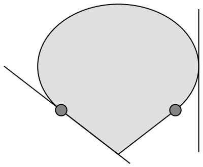
Figure 2: The ellipse with corner is the mean value set $\mathbb{M}(V)$ in Example 1.2 at the angle of $\varphi\approx 0.28\pi$, two tangents are drawn. The proper faces of $\mathbb{M}(V)$ are the extreme points along the closed $3/4$ elliptical arc, the two segments and the point of their intersection. All faces are exposed except the two encircled extreme points.

Let us discuss the mean value set $\mathbb{M}(V)$ for $\varphi>0$. The boundary circle $\partial B$ of $B$ projects to the proper ellipse $e:=\pi_{V}(\partial B)$, the apex $0_{2}\oplus 1$ projects to the point $x:=\pi_{V}(0_{2}\oplus 1)$ and $\mathbb{M}(V)$ is the convex hull of $e$ and $x$. We define for $\alpha\in{\mathbb{R}}$ the unit vector $c(\alpha):=g\cos(\alpha)+h\sin(\alpha)$ in ${\mathbb{R}}^{3}$, so $\partial B$ is parametrized by the states $\rho(\alpha):=\frac{1}{2}({\rm 1\mskip-4.0mul}_{2}+c(\alpha)\widehat{\sigma})\oplus 0$. The coordinate functionals of $v_{1}$ and $v_{2}$ for $a\in{\mathcal{A}}_{\rm sa}$ are $\eta_{i}(a):=\langle v_{i},a\rangle$, $i=1,2$ and for $\alpha\in{\mathbb{R}}$ we have

$$\textstyle\eta_{1}(\rho(\alpha))\;=\;\frac{\cos(\alpha)}{\sqrt{2}}\quad\text{and}\quad\eta_{2}(\rho(\alpha))\;=\;\sin(\alpha)\frac{\sin(\varphi)}{\sqrt{2}}-\frac{\cos(\varphi)}{\sqrt{6}}\,.$$

We write the ellipse $e=\{v\in V\mid\beta(v,v)=0\}$ implicitly with $\beta:{\mathcal{A}}_{\rm sa}\times{\mathcal{A}}_{\rm sa}\to{\mathbb{R}}$

$$\textstyle\beta(a,b)\;:=\;\eta_{1}(a)\eta_{1}(b)+\sin(\varphi)^{-2}[\eta_{2}(a)+\cos(\varphi)/\sqrt{6}\,][\eta_{2}(b)+\cos(\varphi)/\sqrt{6}\,]-\frac{1}{2}$$

and define

$$\textstyle b(\alpha)\;:=\;\beta(0_{2}\oplus 1,\rho(\alpha))\;=\;\frac{1}{2}(\sqrt{3}\cot(\varphi)\cos(\alpha-\frac{\pi}{2})-1)\,.$$

Using the concepts of pole and polar in projective geometry (see e.g. Fischer [Fi]) we have for $\alpha\in{\mathbb{R}}$ that $x$ lies on the tangent to $e$ through $\pi_{V}(\rho(\alpha))$ if and only if $b(\alpha)=0$. The evaluation splits into three cases.

1. If $\frac{\pi}{3}<\varphi\leq\frac{\pi}{2}$, then $\cot(\varphi)<1/\sqrt{3}$ and $b(\alpha)=0$ has no real solution. Thus $x$ lies inside of $e$ and $\mathbb{M}(V)=\operatorname{conv}(e)$.

2. If $\varphi=\frac{\pi}{3}$ then $b(\alpha)=0$ only for $\alpha=\frac{\pi}{2}$. We have $x=\pi_{V}(\rho(\frac{\pi}{2}))=\frac{v_{2}}{\sqrt{6}}\in e$. The generatrix $[0_{2}\oplus 1,\rho(\frac{\pi}{2})]$ of $C$ is perpendicular to $V$ and $\mathbb{M}(V)=\operatorname{conv}(e)$.

3. If $0<\varphi<\frac{\pi}{3}$, then $\cot(\varphi)>1/\sqrt{3}$ and we have $b(\alpha)=0$ for the distinct angles $\alpha=\alpha_{\pm}:=\frac{\pi}{2}\pm\arccos(\tan(\varphi)/\sqrt{3})$. So $\mathbb{M}(V)=\operatorname{conv}(e,x)\supsetneq\operatorname{conv}(e)$. The two tangents of $e$ through $x$ meet $e$ at $\pi_{V}(\rho(\alpha_{\pm}))$. Hence $\pi_{V}(\rho(\alpha_{\pm}))$ are non-exposed extreme points of $\mathbb{M}(V)$.

Two angles are special. For $\varphi=\frac{\pi}{3}$ with $g=(1,0,0)$ and $h=(0,1,0)$ we have $\sqrt{2}\,v_{1}=\sigma_{1}\oplus 0$ and $\sqrt{8/3}\,v_{2}=\sigma_{2}\oplus 1-\frac{{\rm 1\mskip-4.0mul}}{3}$. The drawing in Figure 2 shows $\mathbb{M}(V)$ at $\varphi=\arccos(\sqrt{2/5})\approx 0.28\pi$. Here $g=\frac{1}{\sqrt{2}}(1,-1,0)$ and $h=\frac{1}{\sqrt{2}}(1,1,0)$ give $\sqrt{5/3}\,v_{2}+v_{1}=\sigma_{1}\oplus 1-\frac{{\rm 1\mskip-4.0mul}}{3}$ and $\sqrt{5/3}\,v_{2}-v_{1}=\sigma_{2}\oplus 1-\frac{{\rm 1\mskip-4.0mul}}{3}$. For $\varphi\approx 0.28\pi$ we have $\alpha_{\pm}=\frac{\pi}{2}\pm\frac{\pi}{4}$, so the points $\rho(\alpha_{\pm})$ projecting to the non-exposed faces of $\mathbb{M}(V)$ are orthogonal from the center $\frac{{\rm 1\mskip-4.0mul}_{2}}{2}\oplus 0$ of the base disk $B$. $\Box$

2 Convex geometry of the state space

The facial geometry of state spaces in an infinite-dimensional C*-algebra is well-known, see e.g. Alfsen and Shultz [AS]. We follow the approach of these authors and begin with the cone of positive semi-definite matrices in §2.2. For the finite-dimensional case we write own proofs to make this article self-contained and to address normal cones. In §2.3 we address state spaces and in §2.4 we write a duality for affine sections of self-dual cones.

2.1 Concepts of lattice theory and convex geometry

Let $({\mathbb{E}},\langle\cdot,\cdot\rangle)$ be a finite-dimensional Euclidean vector space. Convex geometric concepts are introduced for subsets of ${\mathbb{E}}$, they can be studied by lattice theory. The main point in this section is the definition of access sequences.

1. They are equivalent to Grünbaum’s [Gr] concept of poonem and to the nowadays more popular notion of face in convex geometry.

2. They were applied by Csiszár and Matúš [CM05] to study mean value sets of statistical models.

3. They will be used in §3.2 to formulate our main result.

Definition 2.1.

A mapping $f:X\to Y$ between two partially ordered sets (posets) $(X,\leq)$ and $(Y,\leq)$ is isotone if for all $x,y\in X$ such that $x\leq y$ we have $f(x)\leq f(y)$. A lattice is a partially ordered set $({\mathcal{L}},\leq)$ where the infimum $x\wedge y$ and supremum $x\vee y$ of each two elements $x,y\in{\mathcal{L}}$ exist. A lattice isomorphism is a bijection between two lattices that preserves the lattice structure. All lattices ${\mathcal{L}}$ appearing in this article are complete, i.e. for an arbitrary subset $S\subset{\mathcal{L}}$ the infimum $\bigwedge S$ and the supremum $\bigvee S$ exist. The least element $\bigwedge{\mathcal{L}}$ and the greatest element $\bigvee{\mathcal{L}}$ in a complete lattice ${\mathcal{L}}$ are improper elements of ${\mathcal{L}}$, all other elements of ${\mathcal{L}}$ are proper elements.$\Box$

Remark 2.2.

For more details on lattices we refer to Birkhoff [Bi]. On face lattices of a convex set see Loewy and Tam or Weis [LT, We].

1. We recall that an isotone bijection between two lattices with an isotone inverse is a lattice isomorphism (see Birkhoff [Bi], §II.3).

2. The reason for completeness of lattices in this article is that they either consist of the faces of a finite-dimensional convex set where a relation $x\lneq y$ always implies a dimension step $\dim(x)<\dim(y)$; or they consist of projections in a finite-dimensional algebra where a relation $x\lneq y$ always implies a rank step $\operatorname{rk}(x)<\operatorname{rk}(y)$. $\Box$

Definition 2.3.

1. The closed segment between $x,y\in{\mathbb{E}}$ is $[x,y]:=\{(1-\lambda)x+\lambda y\mid\lambda\in[0,1]\}$, the open segment is $]x,y[\,:=\{(1-\lambda)x+\lambda y\mid\lambda\in(0,1)\}$. A subset $C\subset{\mathbb{E}}$ is convex if $x,y\in C$ $\implies$ $[x,y]\subset C$. A cone in ${\mathbb{E}}$ is a non-empty subset $C$ closed under non-negative scalar-multiplication, i.e. $\lambda\geq 0,x\in C\implies\lambda x\in C$.

2. Let $C$ be a convex subset of ${\mathbb{E}}$. A face of $C$ is a convex subset $F$ of $C$, such that whenever for $x,y\in C$ the open segment $]x,y[$ intersects $F$, then the closed segment $[x,y]$ is included in $F$. If $x\in C$ and $\{x\}$ is a face, then $x$ is called an extreme point. The set of faces of $C$ will be denoted by ${\mathcal{F}}(C)$, called the face lattice of $C$.

3. The support function of a convex subset $C\subset{\mathbb{E}}$ is defined by ${\mathbb{E}}\to{\mathbb{R}}\cup\{\pm\infty\}$, $u\mapsto h(C,u):=\sup_{x\in C}\langle u,x\rangle$. For non-zero $u\in{\mathbb{E}}$ the set

   $$H(C,u)\;:=\;\{x\in{\mathbb{E}}:\langle u,x\rangle=h(C,u)\}$$

   is an affine hyperplane unless it is empty, which can happen if $C=\emptyset$ or if $C$ is unbounded in $u$-direction. If $C\cap H(C,u)\neq\emptyset$, then we call $H(C,u)$ a supporting hyperplane of $C$. The exposed face of $C$ by $u$ is

   $$F_{\perp}(C,u)\;:=\;C\cap H(C,u)$$

   and we put $F_{\perp}(C,0):=C$. The faces $\emptyset$ and $C$ are exposed faces of $C$ by definition. The set of exposed faces of $C$ will be denoted by ${\mathcal{F}}_{\perp}(C)$, called the exposed face lattice of $C$. A face of $C$, which is not an exposed face is a non-exposed face and we then say the face $F$ is not exposed, see Remark 2.4 (2).

4. If $C\subset{\mathbb{E}}$ is a convex subset, we call a finite sequence $F_{0},\ldots,F_{n}\subset C$ an access sequence (of faces) for $C$ if $F_{0}=C$ and if $F_{i}$ is a proper exposed face of $F_{i-1}$ for $i=1,\ldots,n$,

   $$\textstyle F_{0}\;\supsetneq\;F_{1}\supsetneq\;\cdots\;\supsetneq\;F_{n}\,.$$ (3)

   Grünbaum [Gr] defines a poonem as an element of an access sequence for $C$.

5. Tangency of hyperplanes to a convex subset $C\subset{\mathbb{E}}$ at $x\in C$ is described by the normal cone

   $$\textstyle{\rm N}(C,x)\;:=\;\{u\in{\mathbb{E}}\mid\langle u,y-x\rangle\leq 0\text{ for all }y\in C\,\}\,.$$

6. Some topology is needed. Let $X\subset{\mathbb{E}}$ be an arbitrary subset. The affine hull of $X$, denoted by $\operatorname{aff}(X)$, is the smallest affine subspace of ${\mathbb{E}}$ that contains $X$. The interior of $X$ with respect to the relative topology of $\operatorname{aff}(X)$ is the relative interior $\operatorname{ri}(X)$ of $X$. The complement $X\setminus\operatorname{ri}(X)$ is the relative boundary of $X$. If $C\subset{\mathbb{E}}$ is a non-empty convex subset then we consider the vector space $\operatorname{lin}(C)=\{x-y\mid x,y\in\operatorname{aff}(C)\}$. We define the dimension $\dim(C):=\dim(\operatorname{lin}(C))$ and $\dim(\emptyset):=-1$.$\Box$

Figure 3: A poonem constructed by repeated inclusions of exposed faces.

Remark 2.4.

Let $C\subset{\mathbb{E}}$ be a convex subset.

1. The equivalence of face and poonem is easy to prove, see e.g. Weis [We] §1.2.1. An example of a poonem is depicted in Figure 3.

2. Different to Rockafellar or Schneider [Ro, Sch] we always include $\emptyset$ and $C$ to ${\mathcal{F}}_{\perp}(C)$ so that this is a lattice. The inclusion ${\mathcal{F}}_{\perp}(C)\subset{\mathcal{F}}(C)$ is easy to show. Then by (6) and by the arguments in Remark 2.2 (2) the two lattices ${\mathcal{F}}_{\perp}(C)$ and ${\mathcal{F}}(C)$ ordered by inclusion are complete lattices. An example of non-exposed faces is given in Figure 2.

3. It is easy to show that the normal cone ${\rm N}(C,x)$ is a closed convex cone. For $u\in{\mathbb{E}}$ and $x\in C$ we have

   $$x\in F_{\perp}(C,u)\;\iff\;u\in{\rm N}(C,x)\,.$$ (4)

   This is a fundamental duality and will be picked up in Remark 2.17 (5).

4. Rockafellar [Ro] Thm. 13.1 proves that $x\in{\mathbb{E}}$ belongs to the interior of $C$ if and only if for all non-zero $u\in{\mathbb{E}}$ we have $\langle u,x\rangle<h(C,u)$.

5. We cite a few frequently used relations from Rockafellar [Ro], let $D\subset{\mathbb{E}}$ be a convex subsets. If $\operatorname{ri}(C)\cap\operatorname{ri}(D)\neq\emptyset$, then we have $\operatorname{ri}(C)\cap\operatorname{ri}(D)=\operatorname{ri}(C\cap D)$ by Thm. 6.5. If ${\mathbb{A}}\subset{\mathbb{E}}$ is an affine space and $\alpha:{\mathbb{E}}\to{\mathbb{A}}$ is an affine mapping, then by Thm. 6.6 we have $\alpha(\operatorname{ri}(C))=\operatorname{ri}(\alpha(C))$. Without further assumptions the sum formula $\operatorname{ri}(C)+\operatorname{ri}(D)=\operatorname{ri}(C+D)$ holds by Cor. 6.6.2. If $F$ is a face of $C$ and if $D$ is a (convex) subset of $C$, then by Thm. 18.1 we have

   $$\textstyle\operatorname{ri}(D)\cap F\neq\emptyset\implies D\subset F\,.$$ (5)

   The convex set $C$ admits a partition into relative interiors of its faces

   $$\textstyle C\;=\;\bigcup\limits^{\bullet}{}_{F\in{\mathcal{F}}(C)}\operatorname{ri}(F)$$ (6)

   by Thm. 18.2. In particular, every proper face of $C$ is included in the relative boundary of $C$ and its dimension is strictly smaller than the dimension of $C$. $\Box$

2.2 Positive semi-definite matrices

We recall the well-known convex geometry of the cone of positive semi-definite matrices, see e.g. Ramana and Goldman or Hill and Waters [RG, HW] for real matrices or Alfsen and Shultz [AS] for C*-algebras.

Definition 2.5.

1. The positive semi-definite cone is ${\mathcal{A}}^{+}:=\{a\in{\mathcal{A}}_{\rm sa}\mid a\succeq 0\}$. The self-adjoint matrices are a partially ordered set $({\mathcal{A}}_{\rm sa},\preceq)$ when we define for matrices $a,b\in{\mathcal{A}}_{\rm sa}$ that $a\preceq b$ if and only if $b-a\succeq 0$.

2. A self-adjoint idempotent in ${\mathcal{A}}$ is called a projection. The projection lattice is ${\mathcal{P}}={\mathcal{P}}({\mathcal{A}}):=\{p\in{\mathcal{A}}\mid p=p^{*}=p^{2}\}$.

3. With the identity ${\rm 1\mskip-4.0mul}$ in ${\mathcal{A}}$, the spectrum of a matrix $a\in{\mathcal{A}}$ is ${\rm spec}_{\mathcal{A}}(a):=\{\lambda\in{\mathbb{C}}\mid a-\lambda{\rm 1\mskip-4.0mul}\text{ is not invertible in }{\mathcal{A}}\}$, its elements are the spectral values of $a$ in ${\mathcal{A}}$. A normal matrix $a\in{\mathcal{A}}$ has a unique set of spectral projections $\{p_{\lambda}(a)\}_{\lambda\in{\rm spec}_{\mathcal{A}}(a)}\subset{\mathcal{P}}({\mathcal{A}})$, such that $a=\sum_{\lambda}\lambda p_{\lambda}(a)$ and ${\rm 1\mskip-4.0mul}=\sum_{\lambda}p_{\lambda}(a)$ with summation over $\lambda\in{\rm spec}_{\mathcal{A}}(a)$. The support projection $s(a)$ of $a$ is the sum of all spectral projections $p_{\lambda}(a)$ for non-zero spectral values $\lambda\in{\rm spec}_{\mathcal{A}}(a)$ and the kernel projection of $a$ is $k(a):={\rm 1\mskip-4.0mul}-s(a)$. For a self-adjoint matrix $a$ we denote by $\mu_{+}(a)$ the maximal spectral value of $a$ and by $p_{+}(a)$ the corresponding spectral projection which we call the maximal projection of $a$.

4. The compressed algebra for $p\in{\mathcal{P}}$ is defined by $p{\mathcal{A}}p:=\{pap\mid a\in{\mathcal{A}}\}$.$\Box$

Remark 2.6.

1. For every spectral projection $p$ of a self-adjoint matrix $a\in{\mathcal{A}}_{\rm sa}$ there exists a real polynomial $g$ in one variable, such that $p=g(a)$, see e.g. Brieskorn [Br] Satz 11.19. In particular, this shows $p\in{\mathcal{A}}$.

2. Care should be taken with kernel projections, e.g. $k(0,1)=0$ holds in ${\mathcal{A}}=0\oplus{\mathbb{C}}$ but $k(0,1)=(1,0)$ holds in ${\mathcal{A}}={\mathbb{C}}^{2}$. The maximal projection of $a\in{\mathcal{A}}_{\rm sa}$ has a similar dependence if $\mu_{+}(a)\leq 0$. If several algebras are used simultaneously (e.g. in §3.4) we specify the algebra.

3. The support projection has further characterizations. If $a\in{\mathcal{A}}_{\rm sa}$ is self-adjoint, then $a\in p{\mathcal{A}}p$ $\iff$ $a=pap$ is obvious. Citing [AS] we have

   $$a\;=\;pap \stackrel{{\scriptstyle\text{Lemma 2.20}}}{{\iff}} ap\;=\;a\quad\text{( and equivalently $pa\;=a$ )}$$

   $$\iff s(a)\;\preceq\;p\,.$$

   The last relation holds because the support projection is the least projection such that $as(a)=a$, see [AS] Chap. 2 third section.

4. The ordering $\preceq$ restricts to a partial ordering on ${\mathcal{P}}$. By (3) we have $p\preceq q\iff pq=p$ (or equivalently $qp=p$) for $p,q\in{\mathcal{P}}$. The projection lattice ${\mathcal{P}}$ is a complete lattice with smallest element $0$ and greatest element ${\rm 1\mskip-4.0mul}$. This follows from Remark 2.2 (2).

5. For positive semi-definite matrices $a,b\in{\mathcal{A}}^{+}$ we have three orthogonality conditions. Citing Alfsen and Shultz [AS] these are

   $$\langle a,b\rangle\;=\;0 \iff ab\;=\;0$$

   $$\stackrel{{\scriptstyle\text{Cor.~{}3.6}}}{{\iff}} s(a)s(b)\;=\;0\,.$$

   Here $\operatorname{tr}(ab)=\operatorname{tr}(\sqrt{a}\sqrt{b})(\sqrt{a}\sqrt{b})^{*}$ holds so the orthogonality $\operatorname{tr}(ab)=0$ implies $\sqrt{a}\sqrt{b}=0$ hence $ab=0$. $\Box$

Proposition 2.7.

The positive semi-definite cone ${\mathcal{A}}^{+}$ is a closed convex cone with affine hull and translation vector space equal to ${\mathcal{A}}_{\rm sa}$. The support function satisfies $h({\mathcal{A}}^{+},a)<\infty$ if and only if $a\in-{\mathcal{A}}^{+}$ (and then $h({\mathcal{A}}^{+},a)=0$). The relative interior of ${\mathcal{A}}^{+}$ consists of all positive semi-definite invertible matrices. If $a\in-{\mathcal{A}}^{+}$, then the exposed face of $a$ is the positive semi-definite cone $F_{\perp}({\mathcal{A}}^{+},a)=(k(a){\mathcal{A}}k(a))^{+}$ of the compressed algebra $k(a){\mathcal{A}}k(a)$.

Proof: The positive semi-definite cone consists of all matrices $a\in{\mathcal{A}}_{\rm sa}$, such that for all $u\in{\mathcal{H}}$ we have $\langle u,a(u)\rangle\geq 0$ and therefore it is a closed convex cone. Every self-adjoint matrix $a\in{\mathcal{A}}_{\rm sa}$ is written $a=a^{+}-a^{-}$ for $a^{+},a^{-}\in{\mathcal{A}}^{+}$. This follows from the spectral decomposition of $a$. So the affine hull of ${\mathcal{A}}^{+}$ is ${\mathcal{A}}_{\rm sa}$ and $\operatorname{lin}({\mathcal{A}}^{+})={\mathcal{A}}_{\rm sa}$.

The support function of a convex cone is either $0$ or $\infty$. If $a,b\in{\mathcal{A}}^{+}$ then $\langle-a,b\rangle=-\operatorname{tr}(\sqrt{a}\,b\,\sqrt{a})\leq 0$ holds, so $h({\mathcal{A}}^{+},a)=0$ for all $a\in-{\mathcal{A}}^{+}$. Conversely, if $a\in{\mathcal{A}}_{\rm sa}\setminus(-{\mathcal{A}}^{+})$ then the maximal spectral value of $a$ is positive, thus

$$\textstyle h({\mathcal{A}}^{+},a)\;=\;\sup_{b\in{\mathcal{A}}^{+}}\langle a,b\rangle\;\geq\;\sup_{\lambda\geq 0}\langle a,\lambda p_{+}(a)\rangle\;=\;+\infty\,.$$

We calculate the interior of ${\mathcal{A}}^{+}$ from the support function using Remark 2.4 (4). If $a\not\in-{\mathcal{A}}^{+}$ then $\langle a,b\rangle<h({\mathcal{A}}^{+},a)=\infty$ is trivial for all $a\in{\mathcal{A}}_{\rm sa}$ so it remains to find those $b\in{\mathcal{A}}_{\rm sa}$ where $\langle a,b\rangle>0$ holds for all non-zero $a\in{\mathcal{A}}^{+}$. A necessary condition is that $b$ is positive semi-definite and invertible: indeed, if $p_{\lambda}$ is the spectral projection of $b\in{\mathcal{A}}_{\rm sa}$ for the spectral value $\lambda$ of $b$, then $\lambda\operatorname{rk}(p_{\lambda})=\langle p_{\lambda},b\rangle>0$ so $\lambda>0$. For sufficiency let $\lambda>0$ denote the smallest spectral value of the positive semi-definite invertible matrix $b$. Then

$$\textstyle\langle a,b\rangle\;=\;\operatorname{tr}({\sqrt{a}\,b\,\sqrt{a}})\;\geq\;\operatorname{tr}({\sqrt{a}\,\lambda{\rm 1\mskip-4.0mul}\,\sqrt{a}})\;=\;\lambda\operatorname{tr}(a)\;>\;0\,.$$

To compute for $a\in-{\mathcal{A}}^{+}$ the exposed face $F_{\perp}({\mathcal{A}}^{+},a)$ we have to characterize all $b\in{\mathcal{A}}^{+}$ such that $\langle a,b\rangle=0$. This condition is by (5) equivalent to $s(a)s(b)=0$ and by (3) this is $s(b)\preceq k(a)$ or equivalently $b\in(k(a){\mathcal{A}}k(a))^{+}$. $\Box$

We study tangency of hyperplanes. The following includes the well-known self-duality ${\rm N}({\mathcal{A}}^{+},0)=-{\mathcal{A}}^{+}$ of ${\mathcal{A}}^{+}$, see e.g. Hill and Waters [HW].

Corollary 2.8.

The normal cone of ${\mathcal{A}}^{+}$ at $b\in{\mathcal{A}}^{+}$ is ${\rm N}({\mathcal{A}}^{+},b)=-(k(b){\mathcal{A}}k(b))^{+}$.

Proof: By duality (4) a vector $a\in{\mathcal{A}}_{\rm sa}$ belongs to ${\rm N}({\mathcal{A}}^{+},b)$ if and only if $b\in F_{\perp}({\mathcal{A}}^{+},a)$. Prop. 2.7 says this is equivalent with both $a\in-{\mathcal{A}}^{+}$ and $s(b)\preceq k(a)$ being true. The latter is trivially equivalent to $s(a)\preceq k(b)$, which is by (3) equivalent to $a\in k(b){\mathcal{A}}k(b)$. $\Box$

2.3 The state space

In this section we recall convex geometry of the state space $\mathbb{S}$ including the normal cones. The faces of $\mathbb{S}$ are described in the C*-algebra context by Alfsen and Shultz [AS] Chap. 3 Sec. 1. For every orthogonal projection $p\in{\mathcal{P}}({\mathcal{A}})$ we set

$$\textstyle{\mathbb{F}}(p)\;=\;{\mathbb{F}}_{\mathcal{A}}(p)\;:=\;\mathbb{S}(p{\mathcal{A}}p)$$

and we denote the face lattice of the state space by ${\mathcal{F}}={\mathcal{F}}({\mathcal{A}})$.

Proposition 2.9.

The state space $\mathbb{S}$ is a convex body of dimension $\dim({\mathcal{A}}_{\rm sa})-1$, the affine hull is $\operatorname{aff}(\mathbb{S})={{\mathcal{A}}_{1}}$, the translation vector space is $\operatorname{lin}(\mathbb{S})={{\mathcal{A}}_{0}}$ and the relative interior consists of all invertible states. The support function at $a\in{\mathcal{A}}_{\rm sa}$ is the maximal spectral value $h(\mathbb{S},a)=\mu_{+}(a)$ of $a$. If $a\in{\mathcal{A}}_{\rm sa}$ is non-zero, then the exposed face of $a$ is the state space $F_{\perp}(\mathbb{S},a)={\mathbb{F}}(p)$ of the compressed algebra $p{\mathcal{A}}p$, where $p=p_{+}(a)$ is the maximal projection of $a$.

Proof: The relative interior of the positive semi-definite cone ${\mathcal{A}}^{+}$ consists of the positive semi-definite invertible matrices by Prop. 2.7. It intersects the affine space ${{\mathcal{A}}_{1}}$ of trace-one matrices in the trace state ${\rm 1\mskip-4.0mul}/\operatorname{tr}({\rm 1\mskip-4.0mul})$, so $\operatorname{ri}(\mathbb{S})=\operatorname{ri}({\mathcal{A}}^{+})\cap\operatorname{ri}({{\mathcal{A}}_{1}})$ consists of all invertible states. Since $\operatorname{ri}({\mathcal{A}}^{+})$ is open in ${\mathcal{A}}_{\rm sa}$ the invertible states $\operatorname{ri}(\mathbb{S})$ are an open subset in ${{\mathcal{A}}_{1}}$. We get $\operatorname{aff}(\mathbb{S})={{\mathcal{A}}_{1}}$ and the translation vector space consists of all self-adjoint traceless matrices $\operatorname{lin}(\mathbb{S})={{\mathcal{A}}_{0}}$. The dimension formula follows.

Let us calculate the support function of the state space. We first restrict to vectors $a\in-({\mathcal{A}}^{+}\setminus\operatorname{ri}({\mathcal{A}}^{+}))$. So $a$ is not invertible and $h(\mathbb{S},a)\leq h({\mathcal{A}}^{+},a)=0$ by Prop. 2.7. The state $k(a)/\operatorname{tr}(k(a))$ lies on the supporting hyperplane $H({\mathcal{A}}^{+},a)$ and in $\mathbb{S}$, so $h({\mathcal{A}}^{+},a)=\langle a,k(a)/\operatorname{tr}(k(a))\rangle\leq h(\mathbb{S},a)$ and we get $h(\mathbb{S},a)=0$. For arbitrary $a\in{\mathcal{A}}_{\rm sa}$ we write $a=\mu_{+}(a){\rm 1\mskip-4.0mul}-(\mu_{+}(a){\rm 1\mskip-4.0mul}-a)$, then from $\mathbb{S}\subset{{\mathcal{A}}_{1}}$ we obtain $h(\mathbb{S},a)=\mu_{+}(a)$.

Let us calculate the exposed face $F_{\perp}(\mathbb{S},a)$ for a non-zero vector $a\in-({\mathcal{A}}^{+}\setminus\operatorname{ri}({\mathcal{A}}^{+}))$ first. We have

$$F_{\perp}(\mathbb{S},a)\;=\;{\mathcal{A}}^{+}\cap{{\mathcal{A}}_{1}}\cap H({\mathcal{A}}^{+},a)\;=\;F_{\perp}({\mathcal{A}}^{+},a)\cap{{\mathcal{A}}_{1}}\;\stackrel{{\scriptstyle\text{Prop.~{}\ref{ss:cone}}}}{{=}}\;(k(a){\mathcal{A}}k(a))^{+}\cap{{\mathcal{A}}_{1}}\,.$$

Since $k(a)$ is the maximal projection $k(a)=p_{+}(a)$, we have $F_{\perp}(\mathbb{S},a)=\mathbb{S}(p_{+}(a){\mathcal{A}}p_{+}(a))$. By invariance of the latter formula under substitution $a\mapsto a+\lambda{\rm 1\mskip-4.0mul}$ for real $\lambda$, the formula is true for all non-zero vectors $a\in{\mathcal{A}}_{\rm sa}$. $\Box$

In the C*-algebra context the following isomorphism is proved by Alfsen and Shultz [AS] Cor. 3.36.

Corollary 2.10.

All faces of the state space $\mathbb{S}$ are exposed. The mapping ${\mathbb{F}}:{\mathcal{P}}\to{\mathcal{F}}$, $p\mapsto{\mathbb{F}}(p)$ is an isomorphism of complete lattices.

Proof: For $p\in{\mathcal{P}}\setminus\{0\}$ we have $F_{\perp}(\mathbb{S},p)={\mathbb{F}}(p)$ by Prop. 2.9 and the relative interior is $\operatorname{ri}({\mathbb{F}}(p))=\{\rho\in\mathbb{S}\mid s(\rho)=p\}$. The relative interiors $\operatorname{ri}({\mathbb{F}}(p))$ for non-zero $p\in{\mathcal{P}}$ cover the state space because the support projector of any $\rho\in\mathbb{S}$ lies in ${\mathcal{P}}$ by Rem. 2.6 (1). So ${\mathbb{F}}$ is onto by the decomposition (6) and all faces of $\mathbb{S}$ are exposed. Injectivity of ${\mathbb{F}}$ follows because for $p\neq 0$ the face ${\mathbb{F}}(p)$ contains $p/\operatorname{tr}(p)$ in its relative interior and no $q/\operatorname{tr}(q)$ for any other non-zero $q\in{\mathcal{P}}$. The mappings ${\mathbb{F}}$ and ${\mathbb{F}}^{-1}$ are isotone by (3), hence they are lattice isomorphism. The lattices are complete, see Remark 2.2 (2) or Rem. 2.6 (4). $\Box$

We study tangency of hyperplanes.

Proposition 2.11.

The normal cone of $\mathbb{S}$ at $\rho\in\mathbb{S}$ is ${\rm N}(\mathbb{S},\rho)=\{a\in{\mathcal{A}}_{\rm sa}\mid p_{+}(a)\succeq s(\rho)\}$. The relative interior is $\operatorname{ri}({\rm N}(\mathbb{S},\rho))=\{a\in{\mathcal{A}}_{\rm sa}\mid p_{+}(a)=s(\rho)\}$.

Proof: Let $\rho\in\mathbb{S}$. For $a\in{\mathcal{A}}_{\rm sa}$ the duality (4) of normal cones and exposed faces is $a\in{\rm N}(\mathbb{S},\rho)\iff\rho\in F_{\perp}(\mathbb{S},a)$. By Prop. 2.9 the latter is equivalent to $s(\rho)\preceq p_{+}(a)$ proving the first assertion. Let us relate normal cones of $\mathbb{S}$ to these of the positive semi-definite cone ${\mathcal{A}}^{+}$ in Cor. 2.8. We have $a\in{\rm N}({\mathcal{A}}^{+},\rho)$ if and only if $a\in-{\mathcal{A}}^{+}$ and $s(a)\preceq k(\rho)$. This is trivially equivalent to $a\in-{\mathcal{A}}^{+}$ and $p_{+}(a)\succeq s(\rho)$. So ${\rm N}(\mathbb{S},\rho)={\rm N}({\mathcal{A}}^{+},\rho)+{\mathbb{R}}{\rm 1\mskip-4.0mul}$ follows and $\operatorname{ri}({\rm N}(\mathbb{S},\rho))=\operatorname{ri}({\rm N}({\mathcal{A}}^{+},\rho))+{\mathbb{R}}{\rm 1\mskip-4.0mul}$. By Prop. 2.7 the relative interior of ${\rm N}({\mathcal{A}}^{+},\rho)$ consists of the matrices $a\in-{\mathcal{A}}^{+}$ with $s(a)=k(\rho)$ the latter being trivially equivalent to $p_{+}(a)=s(\rho)$. Adding multiples of ${\rm 1\mskip-4.0mul}$ proves the second assertion. $\Box$

2.4 Dual convex support

We write a convex duality between mean value sets and affine sections of state spaces. This follows from a more general duality between affine sections of a self-dual cone and projections of bases of that cone. The rest of this paper is independent of the results in this section.

Previous work on duality of spectrahedra include Ramana and Goldman or Henrion [RG, He10], see also Rostalski and Sturmfels [RS]. While these authors discuss duality of (not necessarily bounded) spectrahedra in different settings, we depart from a projection of a bounded base of a self-dual cone that generalizes a projection of a state space hence a convex support set. Unlike the projection of an unbounded cone (e.g. the ice-cream cone $\{(x,y,z)\in{\mathbb{R}}^{3}\mid z\geq 0,x^{2}+y^{2}\leq z^{2}\}$ and its orthogonal projection along a generatrix) a sufficiently nice base (affine section of codimension one) of a self-dual convex cone is compact and has a closed projection. Our duality is involutive for a reasonable class.

Let $({\mathbb{E}},\langle\cdot,\cdot\rangle)$ be a finite-dimensional Euclidean vector space. We denote the topological interior of a subset $X\subset{\mathbb{E}}$ by ${\rm int}(X)$. For $x\in{\mathbb{E}}$ we write $x^{\perp}:=\{x\}^{\perp}$.

Definition 2.12.

1. The polar of a subset $C\subset{\mathbb{E}}$ is $C^{\circ}:=\{x\in{\mathbb{E}}\mid\langle x,y\rangle\leq 1\,\forall y\in C\}$ and the dual of $C$ is $C^{*}:=-C^{\circ}=\{x\in{\mathbb{E}}\mid 1+\langle x,y\rangle\geq 0\,\forall y\in C\}$. The set $C$ is self-dual if $C^{**}:=(C^{*})^{*}=C$.

2. The recession cone of a convex subset $C\subset{\mathbb{E}}$ is ${\rm rec}(C)\;:=\;\{\,x\in{\mathbb{E}}\mid C+x\subset C\,\}$.

3. A convex cone $C\subset{\mathbb{E}}$ is salient if $C\cap(-C)=\{0\}$.

4. A base of a convex cone $C\subset{\mathbb{E}}$ is any subset $B\subset C$, such that for all $c\in C$ there exist $\lambda\geq 0$ and $b\in B$ such that $c=\lambda b$ holds. $\Box$
   

Remark 2.13.

1. For a convex subset $C\subset{\mathbb{E}}$ we have $(C^{\circ})^{\circ}=C$ if and only if $C$ is closed and $0\in C$, see e.g. Grünbaum [Gr] §3.4. Equivalently $C^{**}=C$ holds.

2. For a convex cone $C\subset{\mathbb{E}}$ we have $C^{\circ}=\{x\in{\mathbb{E}}\mid\langle x,y\rangle\leq 0\,\forall y\in C\}$. This implies $C^{*}=-{\rm N}(C,0)=\{x\in{\mathbb{E}}\mid\langle x,y\rangle\geq 0\,\forall y\in C\}$ for the normal cone ${\rm N}(C,0)$.

3. If $C\subset{\mathbb{E}}$ is a convex cone and ${\rm int}(C)\neq\emptyset$ then $x\in{\mathbb{E}}$ belongs to ${\rm int}(C)$ if and only if $\langle x,y\rangle>0$ holds for all non-zero $y\in C^{*}$. This follows from the support function $h(C,y)$ having value $0$ if $y\in C^{\circ}$ and $+\infty$ otherwise. Remark 2.4 (4) concludes.

4. It is easy to show that every self-dual convex cone is closed, has non-empty interior and is salient. Also, a convex cone is salient if and only if $0$ is an extreme point.

5. Boundedness of convex sets is described by Rockafellar [Ro] §8 in terms of recession cones. If $C\subset{\mathbb{E}}$ is a non-empty closed convex set, then $C$ is bounded if and only if ${\rm rec}(C)=\{0\}$. If $C\subset{\mathbb{E}}$ is a non-empty closed convex cone, then ${\rm rec}(C)=C$. If $\{C_{i}\}_{i\in I}$ is a family of closed convex subsets of ${\mathbb{E}}$ with non-empty intersection, then ${\rm rec}(\bigcap_{i\in I}C_{i})=\bigcap_{i\in I}{\rm rec}(C_{i})$. $\Box$
   

Lemma 2.14.

Let $C\subset{\mathbb{E}}$ be a self-dual convex cone and let $x\in{\mathbb{E}}$ be non-zero. Then $x\in-C$ if and only if $(x+x^{\perp})\cap C=\emptyset$. The following assertions are equivalent.

1. $x\in{\rm int}(C)$,

2. $\langle x,y\rangle>0$ for all non-zero $y\in C$,

3. $(x+x^{\perp})\cap C$ is a base of $C$,

4. $x\in C$ and $x^{\perp}\cap C=\{0\}$,

5. $(x+x^{\perp})\cap C$ is non-empty and bounded.

Proof: In the first assertion, if $x\in-C$ then for all $y\in C$ and $z\in x+x^{\perp}$ we have $\langle x,y-z\rangle\leq-\|x\|_{2}^{2}$ so $(x+x^{\perp})\cap C=\emptyset$. If $x\not\in-C$ and $x\not\in C$ then by self-duality $C^{*}=C$ there exist $y,z\in C$ such that $\lambda_{y}:=\langle x,y\rangle>0$ and $\lambda_{z}:=\langle x,z\rangle<0$. One obtains $\|x\|_{2}^{2}(2y/\lambda_{y}-z/\lambda_{z})\in(x+x^{\perp})\cap C$.

We prove equivalence of the five assertions. The equivalence 1.$\iff$2. follows from self-duality $C^{*}=C$ and Rem. 2.13 (3). The equivalence 2.$\iff$3. is trivial. The implication 1.$\implies$4. follows with 2. The implication 4.$\implies$5. follows from properties of the recession cone explained in Rem. 2.13 (5): Since $x\in C$ we have ${\rm rec}((x+x^{\perp})\cap C)=x^{\perp}\cap C=\{0\}$.

We prove the implication 5.$\implies$1. indirectly and assume $x\not\in{\rm int}(C)$. Let us also assume $(x+x^{\perp})\cap C\neq\emptyset$, so we must show that $(x+x^{\perp})\cap C$ is unbounded. From the first paragraph we have $x\not\in-C$ hence there exists by self-duality $C^{*}=C$ a (non-zero) vector $y\in C$ such that $\langle x,y\rangle>0$. Since $x\not\in{\rm int}(C)$ there exists by 2. a non-zero vector $z\in C$ such that $\langle x,z\rangle\leq 0$. As $0$ is an extreme point of the salient cone $C$, it lies not on the segment $[y,z]$. This shows that there exists a non-zero $s\in[y,z]\cap x^{\perp}$. Now $s\in x^{\perp}\cap C$ and since $(x+x^{\perp})\cap C\neq\emptyset$ the recession cone $x^{\perp}\cap C={\rm rec}((x+x^{\perp})\cap C)$ is non-zero and the intersection $(x+x^{\perp})\cap C$ is unbounded. $\Box$

Lemma 2.15.

Let $C\subset{\mathbb{E}}$ be a self-dual convex cone and let $S$ be a non-empty and bounded affine section of $C$. Then for every base $B$ of $C$ we have $0\in\pi_{\operatorname{lin}(S)}(B)$.

Proof: We define the lift $L:2^{\mathbb{E}}\to 2^{C}$ mapping a subset $X\subset{\mathbb{E}}$ to $L(X):=(X+\operatorname{lin}(S))\cap C$. This lift maps faces of $\pi_{\operatorname{lin}(S)^{\perp}}(C)$ to faces of $C$. A face $F$ of $C$ is of the form $F=L(G)$ for a face $G$ of $\pi_{\operatorname{lin}(S)^{\perp}}(C)$ if and only if $L(F)=F$, see Weis [We] §5. By self-duality $C^{*}=C$ the cone $C$ is salient, i.e. $0$ is an extreme point. As $S$ is bounded its recession cone ${\rm rec}(S)=\{0\}$ is trivial. By Rem. 2.13 (5) this gives $\operatorname{lin}(S)\cap C=\{0\}$ and thus $L(\{0\})=\{0\}$. So $0$ is an extreme point of $\pi_{\operatorname{lin}(S)^{\perp}}(C)$.

Since $0$ is an extreme point of $\pi_{\operatorname{lin}(S)^{\perp}}(C)$ there exists a supporting hyperplane $H$ of $\pi_{\operatorname{lin}(S)^{\perp}}(C)$ at $0$ (see e.g. Rockafellar [Ro] Thm. 11.6). Then $H\oplus\operatorname{lin}(S)$ is a supporting hyperplane of $C$ at $0$. So there exists a non-zero vector in the normal cone ${\rm N}(C,0)$ perpendicular to $H\oplus\operatorname{lin}(S)$. By self-duality $C^{*}=C$ its reflection $x$ belongs to $C$. Now $x\in\operatorname{lin}(S)^{\perp}$ shows that $\operatorname{lin}(S)^{\perp}$ must intersect the base $B$ and completes the proof. $\Box$

Theorem 2.16.

Let $C\subset{\mathbb{E}}$ be a self-dual convex cone and $S$ be an affine section of $C$ meeting ${\rm int}(C)$. Let $x\in{\rm int}(C)\cap S$ and put $B:=(x+x^{\perp})\cap C$. Then

$$\textstyle S-x\;=\;\|x\|_{2}^{2}\cdot\pi_{\operatorname{lin}(S)}(B)^{*}\,.$$

If $S$ is bounded then

$$\textstyle\pi_{\operatorname{lin}(S)}(B)\;=\;\|x\|_{2}^{2}\cdot(S-x)^{*}\,.$$

(The duals are calculated in the Euclidean vector space $\operatorname{lin}(S)\subset{\mathbb{E}}$.)

Proof: Lemma 2.14 shows that $B=(x+x^{\perp})\cap C$ is a base of $C$. Then we have

$$\begin{array}[]{rcl}S-x&=&\{\,y\in\operatorname{lin}(S)\mid x+y\in C\,\}\;=\;\{\,y\in\operatorname{lin}(S)\mid\langle x+y,b\rangle\geq 0\;\forall b\in B\,\}\\ &=&\{\,y\in\operatorname{lin}(S)\mid\|x\|_{2}^{2}+\langle y,s\rangle\geq 0\;\forall s\in\pi_{\operatorname{lin}(S)}(B)\,\}\\ &=&\|x\|_{2}^{2}\cdot\{\,y\in\operatorname{lin}(S)\mid 1+\langle y,s\rangle\geq 0\;\forall s\in\pi_{\operatorname{lin}(S)}(B)\,\}\,.\end{array}$$

The second assertion follows from Rem. 2.13 (1) if we have $0\in\pi_{\operatorname{lin}(S)}(B)$. Under the assumption that $S$ is bounded this follows from Lemma 2.15. $\Box$

Remark 2.17.

1. We give for ${\mathbb{E}}:={\mathbb{R}}^{2}$ two examples in the positive quadrant $C:=\{(x,y)\in{\mathbb{R}}^{2}\mid x,y\geq 0\}$ where the duality in Thm. 2.16 is not involutive. If $S:=\{(\lambda,\lambda)\mid\lambda\geq 0\}$ and $x:=(1,1)$, then the base $B$ is the interval $[(2,0),(0,2)]$ and $\pi_{\operatorname{lin}(S)}(B)$ has only the element $(1,1)$. If $\widetilde{S}:=S+(0,1)$, $\widetilde{x}:=(1,2)$ and $\widetilde{B}:=(\widetilde{x}+\widetilde{x}^{\perp})\cap C$, then $\pi_{\operatorname{lin}(\widetilde{S})}(\widetilde{B})$ is the segment between $(\frac{5}{4},\frac{5}{4})$ and $(\frac{5}{2},\frac{5}{2})$.

2. We can coordinize Thm. 2.16. If $F_{0}\in{\rm int}(C)$ and $F_{i}\in{\mathbb{E}}$ for $i=1,\ldots,k$ then we put $F:{\mathbb{R}}^{k}\to{\mathbb{E}}$, $x\mapsto F_{0}+\sum_{i=1}^{k}x_{i}F_{i}$. Using $\widetilde{B}:=(F_{0}+F_{0}^{\perp})\cap C$, a calculation similar to the theorem shows

   $$\textstyle\{x\in{\mathbb{R}}^{k}\mid F(x)\in C\}\;=\;\|F_{0}\|^{2}\cdot\{\langle F_{i},b\rangle_{i=1}^{k}\mid b\in\widetilde{B}\}^{*}\,.$$

   If in addition $\widetilde{S}:=\{F(x)\mid x\in{\mathbb{R}}^{k}\}\cap C$ is bounded then we have $0\in\pi_{\operatorname{lin}(\widetilde{S})}(\widetilde{B})$ by Lemma 2.15. This shows $0\in\{\langle F_{i},b\rangle_{i=1}^{k}\mid b\in\widetilde{B}\}$ and we get

   $$\textstyle\{\langle F_{i},b\rangle_{i=1}^{k}\mid b\in\widetilde{B}\}\;=\;\|F_{0}\|^{2}\cdot\{x\in{\mathbb{R}}^{k}\mid F(x)\in C\}^{*}\,.$$

3. We have in mind the example ${\mathbb{E}}:={\mathcal{A}}_{\rm sa}$ and $C:={\mathcal{A}}^{+}$. The positive semi-definite cone ${\mathcal{A}}^{+}$ is self-dual by Cor. 2.8. We consider $x:=\frac{{\rm 1\mskip-4.0mul}}{\operatorname{tr}({\rm 1\mskip-4.0mul})}$, a subspace of traceless self-adjoint matrices $U\subset{{\mathcal{A}}_{0}}$ and the affine section $S:=(x+U)\cap{\mathcal{A}}^{+}=(x+U)\cap\mathbb{S}$. Then $B=\mathbb{S}$ is the state space, $\operatorname{lin}(S)=U$ and Thm. 2.16 provides

   $$\textstyle U\cap(\mathbb{S}-\frac{{\rm 1\mskip-4.0mul}}{\operatorname{tr}({\rm 1\mskip-4.0mul})})\;=\;\frac{1}{\operatorname{tr}({\rm 1\mskip-4.0mul})}\cdot\mathbb{M}(U)^{*}\quad\text{and}\quad\mathbb{M}(U)\;=\;\frac{1}{\operatorname{tr}({\rm 1\mskip-4.0mul})}\cdot(U\cap(\mathbb{S}-\frac{{\rm 1\mskip-4.0mul}}{\operatorname{tr}({\rm 1\mskip-4.0mul})}))^{*}\,.$$

   With notation from the previous item we set $F_{0}:=\tfrac{{\rm 1\mskip-4.0mul}}{\operatorname{tr}({\rm 1\mskip-4.0mul})}$ and choose traceless self-adjoint matrices $F_{1},\ldots,F_{k}\in{{\mathcal{A}}_{0}}$. Then

   $$\textstyle{\rm cs}(F_{1},\ldots,F_{k})^{*}\;=\;\operatorname{tr}({\rm 1\mskip-4.0mul})\cdot\{x\in{\mathbb{R}}^{k}\mid F(x)\succeq 0\}$$

   and

   $$\textstyle\{x\in{\mathbb{R}}^{k}\mid F(x)\succeq 0\}^{*}\;=\;\operatorname{tr}({\rm 1\mskip-4.0mul})\cdot{\rm cs}(F_{1},\ldots,F_{k})\,.$$

4. Helton and Vinnikov [HV] have introduced the notion of rigid convexity. They have proved that spectrahedra have this strong algebraic and geometric property. Moreover this characterizes two-dimensional spectrahedra. These results apply to convex support sets through the lens of convex duality.

5. A touching cone of a convex set $C$, introduced by Schneider [Sch], can be defined as a non-empty face of a normal cone of $C$. Weis [We] §8 has shown that touching cone generalizes normal cone in an analogous sense as face generalizes exposed face. If $S$ is bounded in Thm. 2.16 then the convex duality induces a lattice isomorphism between the faces of $\pi_{\operatorname{lin}(S)}(B)$ and the touching cones of $S-x$. This restricts to a lattice isomorphism between the exposed faces of $\pi_{\operatorname{lin}(S)}(B)$ and the normal cones of $S-x$. As a result, non-exposed faces of a mean value set can be studied in terms of touching cones of affine sections of state spaces.

6. If the positive semi-definite cone $C={\mathcal{A}}^{+}$ is considered, Henrion [He10] adds to the convex duality in Thm. 2.16 an algebraic duality. The analogue idea describes a convex support set as the convex hull of an algebraic set.$\Box$
   

3 Lattices of the mean value set

Convex support sets have typically non-exposed faces, see Knauf and Weis [KW], Example 1.2 has a whole family. Their existence depends on the projection, the state space itself has only exposed faces by Cor. 2.10. Let $U\subset{\mathcal{A}}_{\rm sa}$ be a subspace. We represent the face lattice of the mean value set $\mathbb{M}(U)$ in §3.1 and §3.2 as a lattice of projections ${\mathcal{P}}_{U}$ in ${\mathcal{A}}$. In §3.3 we calculate ${\mathcal{P}}_{U}$ for an example. In §3.4 we show how to reduce the algebra ${\mathcal{A}}$ if “few” observables are used.

3.1 Inverse projection and exposed faces

We embed face and exposed face lattices of $\mathbb{M}(U)$ into the face lattice ${\mathcal{F}}$ of $\mathbb{S}$ and into the projection lattice ${\mathcal{P}}$ of ${\mathcal{A}}$. We compute the projections for exposed faces of $\mathbb{M}(U)$.

We define for subsets $C\subset{\mathcal{A}}_{\rm sa}$ the (set-valued) lift by

$$L(C)\;=\;L_{U}(C)\;:=\;\mathbb{S}\cap(C+U^{\perp})\,.$$

Restricted to subsets of $\mathbb{M}(U)$ the (set-valued) projection $\pi_{U}$ is left-inverse to the lift $L$. It is not difficult to show for any face $F$ of $\mathbb{M}(U)$ that the lift $L(F)$ is a face of the state space $\mathbb{S}$ (see Weis [We], §5 for the details). We define the

$$\begin{array}[]{lll}&\text{{\it lifted face lattice}}&{\mathcal{L}}_{U}\;=\;{\mathcal{L}}_{U}({\mathcal{A}})\;:=\;\{\,L(F)\,\mid\,F\in{\mathcal{F}}(\mathbb{M}(U))\,\}\\ \text{and}&\text{{\it lifted exposed face lattice}}&{\mathcal{L}}_{U,\perp}\;=\;{\mathcal{L}}_{U,\perp}({\mathcal{A}})\;:=\;\{\,L(F)\,\mid\,F\in{\mathcal{F}}_{\perp}(\mathbb{M}(U))\,\}\,.\end{array}$$

The inclusions ${\mathcal{L}}_{U,\perp}\subset{\mathcal{L}}_{U}\subset{\mathcal{F}}$ hold.

Proposition 3.1 ([We] §5).

The lift $L$ restricts to the bijection ${\mathcal{F}}(\mathbb{M}(U))\stackrel{{\scriptstyle L}}{{\longrightarrow}}{\mathcal{L}}_{U}$ and to the bijection ${\mathcal{F}}_{\perp}(\mathbb{M}(U))\stackrel{{\scriptstyle L}}{{\longrightarrow}}{\mathcal{L}}_{U,\perp}$. These are isomorphisms of complete lattices with inverse $\pi_{U}$. For $u\in U$ we have $\pi_{U}\,[F_{\perp}(\mathbb{S},u)]=F_{\perp}(\mathbb{M}(U),u)$ and $L\,[F_{\perp}(\mathbb{M}(U),u)]=F_{\perp}(\mathbb{S},u)$.

From this proposition we obtain a characterization of the lifted exposed face lattice

$${\mathcal{L}}_{U,\perp}\;=\;\{F_{\perp}(\mathbb{S},u)\mid u\in U\}\cup\{\emptyset\}\,.$$ (9)

We restrict the lattice isomorphism ${\mathbb{F}}^{-1}:{\mathcal{F}}\to{\mathcal{P}}$ in Cor. 2.10 to ${\mathcal{L}}_{U}$ and ${\mathcal{L}}_{U,\perp}$ and assign to $U$ the projection lattice resp. exposed projection lattice

$$\textstyle{\mathcal{P}}_{U}\;=\;{\mathcal{P}}_{U}({\mathcal{A}})\;:=\;{\mathbb{F}}^{-1}(\,{\mathcal{L}}_{U}\,)\qquad\text{resp.}\qquad{\mathcal{P}}_{U,\perp}\;=\;{\mathcal{P}}_{U,\perp}({\mathcal{A}})\;:=\;{\mathbb{F}}^{-1}(\,{\mathcal{L}}_{U,\perp}\,)\,.$$ (10)

Now from (9) and Prop. 2.9 we get:

Corollary 3.2.

The exposed projection lattice is ${\mathcal{P}}_{U,\perp}=\{p_{+}(u)\mid u\in U\}\cup\{0\}$.

3.2 Non-exposed faces

We compute the projections for all faces of $\mathbb{M}(U)$, including non-exposed faces. Our idea is to view a non-exposed face $F$ of the mean value set $\mathbb{M}(U)$ as an exposed face of some other face $G$ of $\mathbb{M}(U)$. Then to represent $G$ as a mean value set in a compressed algebra and to proceed like in §3.1. For $p\in{\mathcal{P}}$ and $a\in{\mathcal{A}}_{\rm sa}$ we put

$$\textstyle c^{p}(a)\;:=\;\pi_{(p{\mathcal{A}}p)_{\rm sa}}(a)\;=\;pap\,.$$ (11)

Lemma 3.3.

If $p\in{\mathcal{P}}$ is a projection, then $c^{p}(U)\stackrel{{\scriptstyle\pi_{U}}}{{\longrightarrow}}\pi_{U}((p{\mathcal{A}}p)_{\rm sa})$ is a real linear isomorphism and the following diagrams commute.

    

Proof: The second and third diagrams follow by restriction from the first diagram. We recall that $\pi_{U}$ and $\pi_{c^{p}(U)}$ are self-adjoint with respect to the Hilbert-Schmidt inner product. The first diagram commutes since we have for $a\in(p{\mathcal{A}}p)_{\rm sa}$ and $u\in U$

$$\langle a-\pi_{U}\circ\pi_{c^{p}(U)}(a),u\rangle\;=\;\langle a-\pi_{c^{p}(U)}(a),u\rangle\;=\;\langle a-\pi_{c^{p}(U)}(a),c^{p}(u)\rangle\;=\;0\,.$$

The top arrow is trivially onto, so is the right upward arrow. The dimension equalities

$$\textstyle\dim\;c^{p}(U)\;=\;\dim\;\pi_{(p{\mathcal{A}}p)_{\rm sa}}(U)\;=\;\dim\;\pi_{U}((p{\mathcal{A}}p)_{\rm sa})$$

hold. Therefore the right upward arrow must be a real linear isomorphism. $\Box$

We connect for $p\in{\mathcal{P}}_{U}$ the projection lattice ${\mathcal{P}}_{U}$ to the projection lattice ${\mathcal{P}}_{c^{p}(U)}(p{\mathcal{A}}p)$. It is easy to show that a face $F\in{\mathcal{F}}$ of the state space $\mathbb{S}$ belongs to the lifted face lattice ${\mathcal{L}}_{U}$ if and only if

$$F\;=\;\mathbb{S}\cap(F+U^{\perp})\,.$$ (12)

Using the lattice isomorphisms in Cor. 2.10, a projection $p\in{\mathcal{P}}$ belongs to the projection lattice ${\mathcal{P}}_{U}$ if and only if

$${\mathbb{F}}(p)\;=\;\mathbb{S}\cap({\mathbb{F}}(p)+U^{\perp})\,.$$ (13)

Orthogonal complements may be calculated in different algebras. If $p\in{\mathcal{P}}$ is an orthogonal projection, we denote by ${}^{\perp_{p}}$ the orthogonal complement in the self-adjoint part $(p{\mathcal{A}}p)_{\rm sa}$ of the compression $p{\mathcal{A}}p$. We apply a modular law like identity for affine spaces. Let ${\mathbb{A}}$ be an affine subspace of the linear space ${\mathbb{E}}$. If $X,Y\subset{\mathbb{E}}$ and if $X$ is included in the translation vector space $\operatorname{lin}({\mathbb{A}})$ of ${\mathbb{A}}$, then we have

$$X+(Y\cap{\mathbb{A}})\;=\;(X+Y)\cap{\mathbb{A}}\,.$$ (14)

Detailed proofs of (12) and (14) are written in [We], §5.

Proposition 3.4.

If $p\in{\mathcal{P}}_{U}$ is a non-zero projection and $M\subset{\mathbb{F}}(p)$ is a subset, then

$${\mathbb{F}}(p)\cap\left(M+c^{p}(U)^{\perp_{p}}\right)\;=\;\mathbb{S}\cap\left(M+U^{\perp}\right)\,.$$

Proof: First we show for every $p\in{\mathcal{P}}$ the equation $c^{p}(U)^{\perp_{p}}=U^{\perp}\cap(p{\mathcal{A}}p)_{\rm sa}$. Both sides of this equation are included in $(p{\mathcal{A}}p)_{\rm sa}$, we choose $a\in(p{\mathcal{A}}p)_{\rm sa}$ and apply Lemma 3.3. We have

$$\textstyle a\in c^{p}(U)^{\perp_{p}}\;\iff\;\pi_{c^{p}(U)}(a)=0\;\iff\;\pi_{U}(a)=0\;\iff\;a\in U^{\perp}\,.$$

Now we prove the proposition assuming $p\in{\mathcal{P}}_{U}$ is non-zero. By (13) we have ${\mathbb{F}}(p)=\mathbb{S}\cap({\mathbb{F}}(p)+U^{\perp})$. If we intersect this equation on both sides with $M+U^{\perp}$ then we get (using $M\subset{\mathbb{F}}(p)$)

$$\textstyle{\mathbb{F}}(p)\cap(M+U^{\perp})\;=\;\mathbb{S}\cap(M+U^{\perp})\,.$$

We modify the left-hand side of the last equation. Using ${\mathbb{F}}(p)=\operatorname{aff}({\mathbb{F}}(p))\cap{\mathbb{F}}(p)$ and $M-\frac{p}{\operatorname{tr}(p)}\subset\operatorname{lin}({\mathbb{F}}(p))$ and dropping brackets in the modular law (14) we have

$$\textstyle(M+U^{\perp})\cap{\mathbb{F}}(p)\;=\;\left[(M-\frac{p}{\operatorname{tr}(p)})+(U^{\perp}+\frac{p}{\operatorname{tr}(p)})\cap\operatorname{aff}({\mathbb{F}}(p))\right]\cap{\mathbb{F}}(p)$$

$$= \textstyle\left[M+(U^{\perp}\cap\operatorname{lin}\,{\mathbb{F}}(p))\right]\cap{\mathbb{F}}(p)\;=\;\left[M+(U^{\perp}\cap(p{\mathcal{A}}p)_{\rm sa})\right]\cap{\mathbb{F}}(p)\,.$$

In the second equality we have used $\frac{p}{\operatorname{tr}(p)}\in\operatorname{aff}({\mathbb{F}}(p))$, in the third equality we have compared traces. Now the proposition follows from the equation $U^{\perp}\cap(p{\mathcal{A}}p)_{\rm sa}=c^{p}(U)^{\perp_{p}}$ proved in the beginning. $\Box$

Prop. 3.4 and (13) characterize projection lattices in compressions:

Corollary 3.5.

If $p\in{\mathcal{P}}_{U}$ then ${\mathcal{P}}_{c^{p}(U)}(p{\mathcal{A}}p)=\{q\in{\mathcal{P}}_{U}\mid q\preceq p\}$.

We introduce an algebraic counterpart to the access sequences (3). For $a,b\in{\mathcal{A}}_{\rm sa}$ let us agree to write $a\prec b$ in place of $a\preceq b$ and $a\neq b$ as well as $a\succ b$ in place of $a\succeq b$ and $a\neq b$.

Definition 3.6 (Access sequence).

We call a finite sequence $p_{0},\ldots,p_{n}\subset{\mathcal{P}}_{U}$ an access sequence (of projections) for $U$ if $p_{0}={\rm 1\mskip-4.0mul}$ and if $p_{i}$ belongs to the exposed projection lattice ${\mathcal{P}}_{c^{p_{i-1}}(U),\perp}(p_{i-1}{\mathcal{A}}p_{i-1})$ for $i=1,\ldots,n$ and such that

$$\textstyle p_{0}\;\succ\;p_{1}\succ\;\cdots\;\succ\;p_{n}\,.$$

I.e. $p_{0}={\rm 1\mskip-4.0mul}$, $p_{1}\in{\mathcal{P}}_{U,\perp}$ with $p_{1}\prec p_{0}$, $p_{2}\in{\mathcal{P}}_{c^{p_{1}}(U),\perp}(p_{1}{\mathcal{A}}p_{1})$ with $p_{2}\prec p_{1}$, etc.$\Box$

Theorem 3.7.

The lattice isomorphism ${\mathcal{P}}_{U}\stackrel{{\scriptstyle\pi_{U}\circ{\mathbb{F}}}}{{\longrightarrow}}{\mathcal{F}}(\mathbb{M}(U))$ induces a bijection from the set of access sequences of projections for $U$ to the set of access sequences of faces for $\mathbb{M}(U)$. If $(p_{0},\ldots,p_{n})$ is an access sequence of projections, this bijection is defined by $(p_{0},\ldots,p_{n})\longmapsto(\pi_{U}\circ{\mathbb{F}}(p_{0}),\ldots,\pi_{U}\circ{\mathbb{F}}(p_{n}))$.

Proof: The lattice isomorphisms in Cor. 2.10 and Prop. 3.1 define a lattice isomorphism ${\mathcal{P}}_{U}\to{\mathcal{F}}(\mathbb{M}(U))$, where $p\mapsto\pi_{U}\circ{\mathbb{F}}(p)$. So ${\rm 1\mskip-4.0mul}\mapsto\mathbb{M}(U)$ shows $p_{0}={\rm 1\mskip-4.0mul}\iff\pi_{U}\circ{\mathbb{F}}(p)=\mathbb{M}(U)$, correctly.

Let $p,q$ be projections in ${\mathcal{P}}_{U}$. Then $\pi_{U}({\mathbb{F}}(p))$ and $\pi_{U}({\mathbb{F}}(q))$ are faces of the mean value set $\mathbb{M}(U)$ by the above isomorphism. If $q\in{\mathcal{P}}_{c^{p}(U),\perp}(p{\mathcal{A}}p)$, then $\pi_{c^{p}(U)}({\mathbb{F}}(q))$ is an exposed face of the mean value set $\mathbb{M}_{p{\mathcal{A}}p}(c^{p}(U))=\pi_{c^{p}(U)}({\mathbb{F}}(p))$ by construction (10) of the exposed projection lattice. Then the second diagram in Lemma 3.3 shows that $\pi_{U}({\mathbb{F}}(q))$ is an exposed face of $\pi_{U}({\mathbb{F}}(p))$, this because the restricted linear isomorphism $\mathbb{M}_{p{\mathcal{A}}p}(c^{p}(U))\stackrel{{\scriptstyle\pi_{U}}}{{\longrightarrow}}\pi_{U}({\mathbb{F}}(p))$ preserves faces and exposed faces of a convex set.

Conversely let $F,G$ be faces of the mean value set $\mathbb{M}(U)$ and let us assume $F=\pi_{U}({\mathbb{F}}(p))$ and $G=\pi_{U}({\mathbb{F}}(q))$ for projections $p,q\in{\mathcal{P}}_{U}$. If $G$ is an exposed face of $F$, then $q\preceq p$ and $\pi_{c^{p}(U)}({\mathbb{F}}(q))$ is an exposed face of the mean value set $\pi_{c^{p}(U)}({\mathbb{F}}(p))=\mathbb{M}_{p{\mathcal{A}}p}(c^{p}(U))$ by the restricted linear isomorphism in Lemma 3.3. So $\pi_{c^{p}(U)}({\mathbb{F}}(q))=\pi_{c^{p}(U)}({\mathbb{F}}(r))$ for some $r\in{\mathcal{P}}_{c^{p}(U),\perp}(p{\mathcal{A}}p)$. We finish the proof by showing $q=r$. We have $p,q\in{\mathcal{P}}_{U}$ and from Cor. 3.5 we get $q\in{\mathcal{P}}_{c^{p}(U)}(p{\mathcal{A}}p)$. The isomorphism ${\mathcal{P}}_{c^{p}(U)}(p{\mathcal{A}}p)\to{\mathcal{F}}(\mathbb{M}_{p{\mathcal{A}}p}(c^{p}(U))$ gives $q=r$. $\Box$

Corollary 3.8.

A projection $p\in{\mathcal{P}}$ belongs to the projection lattice ${\mathcal{P}}_{U}$ if and only if $p$ belongs to an access sequence of projections for $U$.

Proof: The face lattice of the mean value set $\mathbb{M}(U)$ equals by Rem. 2.4 (1) the set of poonems of $\mathbb{M}(U)$. So the faces are exactly the elements of access sequences of faces for $\mathbb{M}(U)$ and the isomorphism in Thm. 3.7 concludes. $\Box$

Corollary 3.9.

For each two projections $p,q\in{\mathcal{P}}_{U}$ such that $p\preceq q$ there exists an access sequence for $U$ including $p$ and $q$.

Proof: By Thm. 3.7 the projections $p$ and $q$ correspond to faces $F,G$ of $\mathbb{M}(U)$ such that $F\subset G$. We concatenate an access sequence for $\mathbb{M}(U)$ including $G$ with an access sequence for $G$ including $F$ to obtain an access sequence for $\mathbb{M}(U)$ including both $F,G$. Then Thm. 3.7 concludes. $\Box$

Remark 3.10.

If sufficient spectral data of the elements of $U$ is available, then the projection lattice ${\mathcal{P}}_{U}$ can be calculated algebraically. This is done gradually using Cor. 3.2: For every known projection $p$ of ${\mathcal{P}}_{U}$ (starting with $p={\rm 1\mskip-4.0mul}$) we compute within the algebra $p{\mathcal{A}}p$ the maximal projections of $c^{p}(U)$. According to Cor. 3.8 we find all elements of ${\mathcal{P}}_{U}$. Example §3.3 demonstrates this procedure. $\Box$

In applications we are interested in the inverse projection of relative interiors of faces of $\mathbb{M}(U)$. These are independent of the representation of a convex support set as a mean value set in the sense of Rem. 1.1 (3): If $\widetilde{U}:=\pi_{{\mathcal{A}}_{0}}(U)$ then we have for any subset $X\subset\mathbb{S}$

$$\textstyle(X+U^{\perp})\cap\mathbb{S}\;=\;(X+\widetilde{U}^{\perp})\cap\mathbb{S}\,.$$

The proof of this equation is written in [We] §5.

Lemma 3.11.

If $\rho\in\mathbb{S}$, then $\rho\in\operatorname{ri}({\mathbb{F}}(p))+U^{\perp}$ holds for a unique projection $p\in{\mathcal{P}}_{U}$. We have $p=\bigwedge\{q\in{\mathcal{P}}_{U}\mid s(\rho)\preceq q\}$.

Proof: We recall from (6) that $\mathbb{M}(U)$ is partitioned into the relative interiors of its faces. Then the lattice isomorphism ${\mathcal{P}}_{U}\to{\mathcal{F}}(\mathbb{M}(U))$, $p\mapsto\pi_{U}({\mathbb{F}}(p))$ in Thm. 3.7 completes the first assertion.

Second, if $\rho\in\mathbb{S}$ and $F$ is the face of $\mathbb{M}(U)$ with $\pi_{U}(\rho)\in\operatorname{ri}(F)$, then it follows from (5) that for every face $G$ of $\mathbb{M}(U)$ with $\pi_{U}(\rho)\in G$ we have $F\subset G$, so

$$\textstyle F\;=\;\bigcap\{G\in{\mathcal{F}}(\mathbb{M}(U))\mid\pi_{U}(\rho)\in G\}\,.$$

Using the above lattice isomorphism we have $G=\pi_{U}({\mathbb{F}}(q))$ for some $q\in{\mathcal{P}}_{U}$. The condition $\pi_{U}(\rho)\in G$ translates with (13) and (3) into

$$\textstyle\pi_{U}(\rho)\in\pi_{U}({\mathbb{F}}(q))\;\iff\;\rho\in{\mathbb{F}}(q)\;\iff\;s(\rho)\preceq q\,.$$

We have $F=\pi_{U}(p)$ for a unique $p\in{\mathcal{P}}_{U}$ and the second assertion follows from the mentioned lattice isomorphism. $\Box$

3.3 The main example, Part II

Figure 4: Spectral analysis of exposed faces, the abelian case of $\varphi=0$. The maximal eigenvalue is drawn bold, degenerate maximal eigenvalues are marked by a circle. Maximal projections are listed next to their maximal eigenvalues.

We continue Example 1.2 and compute the projection lattice ${\mathcal{P}}_{V}$ for a fixed angle $\varphi\in[0,\frac{\pi}{2}]$. First, let us consider the abelian case of $\varphi=0$. The ONB (2) of $V$ is $v_{1}=1/\sqrt{2}g\widehat{\sigma}\oplus 0$ and $v_{2}=\sqrt{2/3}z$ and it generates an abelian algebra isomorphic to ${\mathbb{C}}^{3}$. For $\alpha\in{\mathbb{R}}$ maximizing the eigenvalues of $\cos(\alpha)v_{1}+\sin(\alpha)v_{2}$ is equivalent to maximizing these of

$$\textstyle\sqrt{2}\cos(\alpha)v_{1}+\sqrt{\frac{2}{3}}\sin(\alpha)v_{2}+\sin(\alpha)\frac{{\rm 1\mskip-4.0mul}}{3}\;=\;\cos(\alpha)\rho(0)-\cos(\alpha)\rho(\pi)+\sin(\alpha)0_{2}\oplus 1\,.$$

The eigenvalues $(\cos(\alpha),-\cos(\alpha),\sin(\alpha))$ are depicted in Figure 4. The maximal projections for $\alpha$ increasing from $0$ to $2\pi$ are

$$\rho(0)\,,\quad\rho(0)+0_{2}\oplus 1\,,\quad 0_{2}\oplus 1\,,\quad\rho(\pi)+0_{2}\oplus 1\,,\quad\rho(\pi)\quad\text{and}\quad{\rm 1\mskip-4.0mul}_{2}\oplus 0\,.$$

These projections together with $0$ and ${\rm 1\mskip-4.0mul}$ are the elements of the exposed projection lattice ${\mathcal{P}}_{V}$. Access sequences do not produce further projections because the triangle $\mathbb{M}(V)$ has only exposed faces.

Second, we consider the non-abelian case of $0<\varphi\leq\frac{\pi}{2}$. Using the ONB (2) of $V$ we carry out the spectral analysis with

$$\textstyle w_{\pm}\;:=\;\frac{v_{2}}{\sin(\varphi)}\pm v_{1}+\frac{\cot(\varphi)}{\sqrt{6}}{\rm 1\mskip-4.0mul}\,.$$

For $\alpha\in{\mathbb{R}}$ and $w(\alpha):=w_{+}\cos(\alpha)+w_{-}\sin(\alpha)$ we have the spectral decomposition

$$\textstyle w(\alpha)\;=\;\rho(\alpha+\frac{\pi}{4})-\rho(\alpha+\frac{5}{4}\pi)+f(\alpha)0_{2}\oplus 1$$ (15)

where $f(\alpha)=\sqrt{3}\cot(\varphi)\cos(\alpha-\frac{\pi}{4})$. The eigenvalues $(1,-1,f(\alpha))$ of $w(\alpha)$ are plotted in Figure 5 for different values of $\varphi$.

Figure 5: Spectral analysis of exposed faces, the non-abelian case of $0<\varphi\leq\frac{\pi}{2}$. The eigenvalues are $(1,-1,f(\alpha))$. At $\alpha=\frac{9}{4}\pi$ the graphs of $f$ correspond to angles of $\varphi=0.3\overline{8}>0.\overline{3}>0.28\ldots>0.\overline{2}$ in units of $\pi$ (from bottom to top).

1. For $\frac{\pi}{3}<\varphi\leq\frac{\pi}{2}$ we have seen in Example 1.2 that $\mathbb{M}(V)$ is an ellipse. We have $\cot(\varphi)<1/\sqrt{3}$ and $f(\alpha)=1$ has no real solution. So for $\alpha\in{\mathbb{R}}$ the maximal projection of $w(\alpha)$ has constant rank one, it is given by the pure state $\rho(\alpha)$. The compressed algebra is $\rho(\alpha){\mathcal{A}}\rho(\alpha)\cong{\mathbb{C}}$ and hence ${\mathcal{P}}_{V}={\mathcal{P}}_{V,\perp}$ consists of the $\rho(\alpha)$’s and of $0$ and ${\rm 1\mskip-4.0mul}$.

For values of $0<\varphi\leq\frac{\pi}{3}$ the equation $f(\alpha)=1$ has solutions, we start with auxiliary calculations first. For $\alpha\in{\mathbb{R}}$ and $x,y\in{\mathbb{R}}^{3}$ we have $\rho(\alpha)(x\widehat{\sigma}\oplus 0)\rho(\alpha)=\rho(\alpha)\langle c(\alpha),x\rangle$ where $\langle\cdot,\cdot\rangle$ is the Euclidean scalar product $\langle x,y\rangle=x_{1}y_{1}+x_{2}y_{2}+x_{3}y_{3}$ on ${\mathbb{R}}^{3}$. The angle $\delta:=\arccos(\tan(\varphi)/\sqrt{3}\,)$ is important, it satisfies $0\leq\delta<\frac{\pi}{2}$ with $\delta=0\iff\varphi=\frac{\pi}{3}$. From the eigenvalue discussion of $w(\alpha)$ in (15) we get that rank-two maximal projections of $w(\alpha)$ appear under the angles of $\alpha=\frac{\pi}{4}\pm\delta$, these are the projections $p_{\pm}:=\rho(\alpha_{\pm})+0_{2}\oplus 1$ for $\alpha_{\pm}:=\frac{\pi}{2}\pm\delta$. In addition, for $\frac{\pi}{4}+\delta<\alpha<\frac{9}{4}\pi-\delta$ the maximal projections of $w(\alpha)$ are $\rho(\widetilde{\alpha})$ for the angles of $\alpha_{+}<\widetilde{\alpha}<2\pi+\alpha_{-}$. For $\sigma\in\{-,+\}$ we begin to calculate $c^{p_{\sigma}}(V)$ finding $p_{\sigma}v_{1}p_{\sigma}=\cos(\alpha_{\sigma})/\sqrt{2}\,\rho(\alpha_{\sigma})$ and $p_{\sigma}v_{2}p_{\sigma}$ is not important now. We notice that the algebra $p_{\sigma}{\mathcal{A}}p_{\sigma}\cong{\mathbb{C}}^{2}$ is abelian, its state space is the segment $[\rho(\alpha_{\sigma}),0_{2}\oplus 1]$.

1. For $\varphi=\frac{\pi}{3}$ we saw in Example 1.2 that the mean value set $\mathbb{M}(V)$ is an ellipse. We have $\delta=0$ so $\alpha_{+}=\alpha_{-}=\frac{\pi}{2}$ and ${\mathcal{P}}_{V,\perp}$ contains a single rank-two projection $p_{\pm}=\rho(\frac{\pi}{2})+0_{2}\oplus 1$. Summing up, the projection lattice ${\mathcal{P}}_{V,\perp}$ consists of $0$, ${\rm 1\mskip-4.0mul}$ the rank-one projections $\rho(\widetilde{\alpha})$ for $\frac{\pi}{2}<\widetilde{\alpha}<\frac{5}{2}\pi$ and of the rank-two projection

   $$\textstyle p_{\pm}\;=\;\rho(\frac{\pi}{2})+0_{2}\oplus 1\,.$$

   We have seen in the auxiliary calculations that $p_{\pm}v_{1}p_{\pm}=0$ and we find $p_{\pm}v_{2}p_{\pm}=p_{\pm}/\sqrt{6}$. Then it follows $c^{p_{\pm}}(V)={\mathbb{R}}p_{\pm}$ and hence we have proved ${\mathcal{P}}_{V}={\mathcal{P}}_{V,\perp}$.

2. For $0<\varphi<\frac{\pi}{3}$ the mean value set $\mathbb{M}(V)$ is an ellipse with a corner. We have $0<\delta<\frac{\pi}{2}$ so $\rho(\alpha_{+})\neq\rho(\alpha_{-})$ and ${\mathcal{P}}_{V,\perp}$ contains the distinct rank-two projections $p_{\pm}:=\rho(\alpha_{\pm})+0_{2}\oplus 1$. For the angles $\frac{\pi}{4}-\delta<\alpha<\frac{\pi}{4}+\delta$ the maximal projection of $w(\alpha)$ is $0_{2}\oplus 1$ so the exposed projection lattice ${\mathcal{P}}_{V,\perp}$ consists of $0$ and ${\rm 1\mskip-4.0mul}$, of $\rho(\widetilde{\alpha})$ for the angles of $\alpha_{+}<\widetilde{\alpha}<2\pi+\alpha_{-}$ and of

   $$p_{-}\;=\;\rho(\alpha_{-})+0_{2}\oplus 1\,,\quad\;0_{2}\oplus 1\,,\quad p_{+}\;=\;\rho(\alpha_{+})+0_{2}\oplus 1\,.$$

   For $\sigma\in\{-,+\}$ we have $\cos(\alpha_{\sigma})\neq 0$ since $0<\delta<\frac{\pi}{2}$. The vector $p_{\sigma}v_{1}p_{\sigma}$ is non-zero proportional to $\rho(\alpha_{\sigma})$, so $\pm\,\rho(\alpha_{\sigma})\in c^{p_{\sigma}}(V)$. The maximal projections within $p_{\sigma}{\mathcal{A}}p_{\sigma}$ are $p_{+}(\rho(\alpha_{\sigma}))=\rho(\alpha_{\sigma})$ and $p_{+}(-\rho(\alpha_{\sigma}))=0_{2}\oplus 1$. The abelian algebra $p_{\sigma}{\mathcal{A}}p_{\sigma}$ has only four orthogonal projections $0$, $\rho(\alpha_{\sigma})$, $0_{2}\oplus 1$ and $p_{\sigma}$. Three of them are already in ${\mathcal{P}}_{V,\perp}$ so the projection lattice ${\mathcal{P}}_{V}$ exceeds ${\mathcal{P}}_{V,\perp}$ by the projections

   $$\rho(\alpha_{-})\quad\text{and}\quad\rho(\alpha_{+})$$

   corresponding to the two non-exposed faces of $\mathbb{M}(V)$.

3.4 Reductions of the state space

If a simplified state space is desired while a given convex support set shall be kept, then (depending on the observables) the algebra can be reduced. An example shows that this is not possible without conditions:

Example 3.12.

Let ${\mathcal{B}}:=\operatorname{Mat}(2,{\mathbb{C}})\oplus{\mathbb{C}}$ and ${\mathcal{C}}:=\operatorname{Mat}(2,{\mathbb{C}})\oplus 0$. Even though the algebra ${\mathcal{C}}$ contains the observables $u_{1}:=(\sigma_{1}-{\rm 1\mskip-4.0mul}_{2})\oplus 0$ and $u_{2}:=(\sigma_{2}-{\rm 1\mskip-4.0mul}_{2})\oplus 0$, reduction of ${\mathcal{B}}$ to ${\mathcal{C}}$ changes the convex support set ${\rm cs}(u_{1},u_{2})$ essentially.

Let $\widetilde{u}_{1}:=\sigma_{1}\oplus 1-\frac{{\rm 1\mskip-4.0mul}}{3}$, $\widetilde{u}_{2}:=\sigma_{2}\oplus 1-\frac{{\rm 1\mskip-4.0mul}}{3}$ and $\widetilde{U}:={\rm span}(\widetilde{u}_{1},\widetilde{u}_{2})$. Then $\mathbb{M}_{\mathcal{B}}(\widetilde{U})$ is the ellipse with corner depicted in Figure 2. Using $U:={\rm span}(u_{1},u_{2})$, Rem. 1.1 provides restricted affine isomorphisms

$$\textstyle\mathbb{M}_{\mathcal{B}}(U)\;\stackrel{{\scriptstyle m}}{{\longrightarrow}}\;{\rm cs}(u_{1},u_{2})\;\stackrel{{\scriptstyle\alpha^{-1}}}{{\longrightarrow}}\;\mathbb{M}_{\mathcal{B}}(\widetilde{U})$$

so $\mathbb{M}_{\mathcal{B}}(U)$ is an ellipse with corner. On the other hand the state space of ${\mathcal{C}}$ is a Bloch ball so the mean value set $\mathbb{M}_{{\mathcal{C}}}(U)$ must be an ellipse, which is not affinely isomorphic to the ellipse with corner $\mathbb{M}_{\mathcal{B}}(U)$.$\Box$

Other reductions of the state space are nevertheless possible. Let $U\subset{\mathcal{A}}_{\rm sa}$ be a subspace. We define a projection as the supremum

$$\textstyle p\;:=\;\bigvee\{s(u)\mid u\in U\,\}\,.$$

Denoting for $n\in{\mathbb{N}}$ the ring of polynomials in $n$ variables $x_{1},\ldots,x_{n}$ over the field $K$ by $K[x_{1},\ldots,x_{n}]$, we define the C*-algebra

$$\textstyle{\mathcal{B}}(U)\;:=\;\{pg(u_{1},\ldots,u_{n})\mid u_{i}\in U,\,i=1,\ldots,n,\,g\in{\mathbb{C}}[x_{1},\ldots,x_{n}],\,n\in{\mathbb{N}}\,\}\,.$$

If ${\mathcal{A}}\subset\operatorname{Mat}(n,{\mathbb{R}})$ for some $n\in{\mathbb{N}}$ (see §1.1) the C*-algebra ${\mathcal{B}}(U)$ may not be included in ${\mathcal{A}}$ so we define

$$\textstyle{\mathcal{R}}(U)\;:=\;\{pg(u_{1},\ldots,u_{n})\mid u_{i}\in U,\,i=1,\ldots,n,\,g\in{\mathbb{R}}[x_{1},\ldots,x_{n}],\,n\in{\mathbb{N}}\,\}\,.$$

We shall make use of Minkowski’s theorem, see e.g. Schneider [Sch] §1.4. This theorem states that every convex body $C$ in a finite-dimensional Euclidean vector space is the convex hull of its extreme points. We recall that ${{\mathcal{A}}_{0}}$ is the space of traceless self-adjoint matrices (see §1.1).

Lemma 3.13.

1. If ${\mathcal{A}}$ is a C*-algebra and if one of the conditions $p={\rm 1\mskip-4.0mul}$ or $U\subset{{\mathcal{A}}_{0}}$ holds, then we have $\mathbb{M}_{\mathcal{A}}(U)=\mathbb{M}_{{\mathcal{B}}(U)}(U)$.

2. If $U\subset\operatorname{Mat}(n,{\mathbb{R}})$ for some $n\in{\mathbb{N}}$ (${\mathcal{A}}$ may be a C*-algebra) and if one of the conditions $p={\rm 1\mskip-4.0mul}$ or $U\subset{{\mathcal{A}}_{0}}$ holds, then we have $\mathbb{M}_{\mathcal{A}}(U)=\mathbb{M}_{{\mathcal{R}}(U)}(U)$.

Proof: The lattice isomorphism ${\mathcal{P}}_{U}\to{\mathcal{F}}(\mathbb{M}(U))$, $p\mapsto\pi_{U}({\mathbb{F}}(p))$ in Thm. 3.7 shows that there is a subset ${\mathcal{P}}_{e}\subset{\mathcal{P}}_{U}$ of projections such that every extreme point of $\mathbb{M}_{\mathcal{A}}(U)$ is of the form $e(p):=\pi_{U}(\frac{p}{\operatorname{tr}(p)})$ for some $p\in{\mathcal{P}}_{e}$. If condition 1. resp. 2. above holds, then by Thm. 3.7 and by Rem. 2.6 (1) we have ${\mathcal{P}}_{e}\subset{\mathcal{B}}(U)$ resp. ${\mathcal{P}}_{e}\subset{\mathcal{R}}(U)$. By Minkowski’s theorem the mean value set $\mathbb{M}_{\mathcal{A}}(U)$ is the convex hull of $\{e(p)\mid p\in{\mathcal{P}}_{e}\}$, so $\mathbb{M}_{\mathcal{A}}(U)\subset\mathbb{M}_{{\mathcal{B}}(U)}(U)$ resp. $\mathbb{M}_{\mathcal{A}}(U)\subset\mathbb{M}_{{\mathcal{R}}(U)}(U)$ follows. The converse inclusion is trivial. $\Box$

Example 3.12 (Continued).

The algebras ${\mathcal{A}}_{\mathbb{C}}:=\operatorname{Mat}(3,{\mathbb{C}})$, ${\mathcal{A}}_{\mathbb{R}}:=\operatorname{Mat}(3,{\mathbb{R}})$, ${\mathcal{B}}_{\mathbb{C}}:=\operatorname{Mat}(2,{\mathbb{C}})\oplus{\mathbb{C}}$ and ${\mathcal{B}}_{\mathbb{R}}:=\operatorname{Mat}(2,{\mathbb{R}})\oplus{\mathbb{R}}$ have the inclusions ${\mathcal{B}}_{\mathbb{R}}\subset{\mathcal{B}}_{\mathbb{C}}\subset{\mathcal{A}}_{\mathbb{C}}$ and ${\mathcal{B}}_{\mathbb{R}}\subset{\mathcal{A}}_{\mathbb{R}}\subset{\mathcal{A}}_{\mathbb{C}}$. The state space of ${\mathcal{A}}_{\mathbb{C}}$ is an eight-dimensional convex body which has three-dimensional Bloch balls as its largest proper faces, the five-dimensional state space $\mathbb{S}({\mathcal{A}}_{\mathbb{R}})$ has two-dimensional disks as its largest proper faces. The state space $\mathbb{S}({\mathcal{B}}_{\mathbb{C}})=\operatorname{conv}(\mathbb{S}(\operatorname{Mat}(2,{\mathbb{C}}))\oplus 0,0_{2}\oplus 1)$ is a four-dimensional cone with a Bloch ball as its base. The state space $\mathbb{S}({\mathcal{B}}_{\mathbb{R}})=\operatorname{conv}(\mathbb{S}(\operatorname{Mat}(2,{\mathbb{R}}))\oplus 0,0_{2}\oplus 1)$ is a three-dimensional cone with a two-dimensional base disk, it is the cone $C$ in Example 1.2 for $W={\rm span}(\sigma_{1}\oplus 0,\sigma_{3}\oplus 0)$. While the dimensions of the algebras $8>5>4>3$ decrease, their mean value sets $\mathbb{M}_{{\mathcal{A}}_{{\mathbb{C}}}}(U)=\mathbb{M}_{{\mathcal{A}}_{{\mathbb{R}}}}(U)=\mathbb{M}_{{\mathcal{B}}_{{\mathbb{C}}}}(U)=\mathbb{M}_{{\mathcal{B}}_{{\mathbb{R}}}}(U)$ coincide by Lemma 3.13. This equality extends $\mathbb{M}_{{\mathcal{B}}_{{\mathbb{C}}}}(U)=\mathbb{M}_{{\mathcal{B}}_{{\mathbb{R}}}}(U)$ in (1.2).$\Box$

Remark 3.14.

1. Of course $\mathbb{M}_{\mathcal{A}}(U)=\mathbb{M}_{{\mathcal{C}}}(U)$ would follow if we use any complex or real algebra ${\mathcal{C}}$ in case 1. of Lemma 3.13 such that ${\mathcal{B}}(U)\subset{\mathcal{C}}\subset{\mathcal{A}}$ or in case 2. such that ${\mathcal{R}}(U)\subset{\mathcal{C}}\subset{\mathcal{A}}$.

2. Thm. 3.7 is not necessary to prove Lemma 3.13. We may also use Straszewicz’s theorem (see e.g. Schneider [Sch] §1.4: The exposed extreme points of a convex body are dense in the set of its extreme points.) together with Cor. 3.2. $\Box$

Acknowledgment. I whish to thank Andreas Knauf and Markus Müller for fruitful discussions. I am grateful to Didier Henrion for enriching discussions at the “Course on LMI Optimization” in March 2011 at Czech Technical University, Prague, and to the group of Zdeněk Hurák for their hospitality there.

References

- [AS] E. M. Alfsen and F. W. Shultz, State Spaces of Operator Algebras, Birkhäuser (2001).
- [Am] S. Amari, Information Geometry on Hierarchy of Probability Distributions, IEEE Trans. Inf. Theory vol. 47 no. 5 1701–1711 (2001).
- [AN] S. Amari and H. Nagaoka, Methods of Information Geometry, Translations of Mathematical Monographs vol. 191 (2000).
- [Ay] N. Ay, An Information-Geometric Approach to a Theory of Pragmatic Structuring, Ann. Probab. vol. 30 416–436 (2002).
- [AK] N. Ay and A. Knauf, Maximizing Multi-Information, Kybernetika vol. 42 no. 5 517–538 (2006).
- [Ba] O. Barndorff-Nielsen, Information and Exponential Families in Statistical Theory, John Wiley & Sons, Ltd (1978).
- [BN] A. Ben-Tal and A. Nemirovski, Lectures on Modern Convex Optimization, MPS/SIAM Series on Optimization (2001).
- [BZ] I. Bengtsson and K. Życzkowski, Geometry of Quantum States. An Introduction to Quantum Entanglement, Cambridge University Press (2006).
- [Bi] G. Birkhoff, Lattice Theory, 3rd ed. AMS Colloquium Publications (1973).
- [Br] E. Brieskorn, Lineare Algebra und Analytische Geometrie II, Vieweg (1982).
- [CM03] I. Csiszár and F. Matúš, Information Projections Revisited, IEEE Trans. Inf. Theory vol. 49 1474–1490 (2003).
- [CM05] I. Csiszár and F. Matúš, Closures of Exponential families, Ann. Probab. vol. 33 no. 2 582–600 (2005).
- [Da] K. R. Davidson, C*-Algebras by Example, Fields Institute Monographs vol. 6 (1996).
- [Do] A. C. Doherty, P. A. Parrilo and F. M. Spedalieri, Complete Family of Separability Criteria, Phys. Rev. A vol. 69 (2004).
-
[DZ]
C. F. Dunkl, P. Gawron, J. A. Holbrook,
J. A. Miszczak, Z. Puchała and K. Życzkowski,
Numerical shadow and geometry of quantum states,
http://arxiv.org/abs/1104.2760(2011). - [Fi] G. Fischer, Analytische Geometrie, Vieweg (1985).
- [Gr] B. Grünbaum, Convex Polytopes, 2nd ed. Springer-Verlag (2003).
- [Ha] W. Hall, Compatibility of Subsystem States and Convex Geometry, Phys. Rev. A vol. 75 (2007).
- [HV] G. W. Helton and V. Vinnikov, Linear Matrix Inequality Representation of Sets, Comm. Pure Appl. Math. vol. LX 0654–0674 (2007).
- [He10] D. Henrion, Semidefinite Geometry of the Numerical Range, El. J. of Lin. Alg. vol. 20 322-332 (2010).
-
[He11]
D. Henrion, Semidefinite Representation of
Convex Hulls of Rational Varieties,
http://arxiv.org/abs/0901.1821(2011). - [HW] R. D. Hill and S. R. Waters, On the Cone of Positive Semidefinite Matrices, Lin. Alg. Appl. vol. 90 81–88 (1987).
- [Ho] A. S. Holevo, Probabilistic and Statistical Aspects of Quantum Theory, 2nd ed. Edizioni Della Normale (2011).
- [In] R. S. Ingarden, A. Kossakowski and M. Ohya, Information Dynamics and Open Systems, Kluwer Academic Publishers (1997).
-
[Ja]
P. Janotta, C. Gogolin, J. Barrett
and N. Brunner, Limits on Non-Local Correlations From the Structure
of the Local State Space,
http://arxiv.org/abs/1012.1215(2011). -
[KW]
A. Knauf and S. Weis, Entropy Distance:
New Quantum Phenomena,
http://arxiv.org/abs/1007.5464(2010). - [Ko] M. Kojima, S. Kojima and S. Hara, Linear Algebra for Semidefinite Programming, Sūrikaisekikenkyūsho Kōkyūroku vol. 1004 (1997).
- [LT] R. Loewy and B. Tam, Complementation in the Face Lattice of a Proper Cone, Lin. Alg. Appl. vol. 79 195–206 (1986).
- [Mu] G. J. Murphy, C*-Algebras and Operator Theory, Academic Press Inc. (1990).
- [My] G. O. Myhr, J. M. Renes, A. C. Doherty and N. Lütkenhaus, Symmetric Extension in Two-Way Quantum Key Distribution, Phys. Rev. A vol. 79 (2009).
- [NC] M. A. Nielsen and I L. Chuang, Quantum Computation and Quantum Information, Cambridge University Press (2000).
-
[Pe]
D. Petz,
Quantum Information Theory and Quantum Statistics,
Springer-Verlag (2008). - [RG] M. Ramana and A. J. Goldman, Some Geometric Results in Semidefinite Programming, Journal of Global Optimization vol. 7 33–50 (1995).
- [Ro] R. T. Rockafellar, Convex Analysis, Princeton University Press (1972).
-
[RS]
P. Rostalski and B. Sturmfels,
Dualities in Convex Algebraic Geometry,
http://arxiv.org/abs/1006.4894(2010). - [Ru] D. Ruelle, Statistical Mechanics: Rigorous Results, World Scientific (1999).
- [Sch] R. Schneider, Convex Bodies: The Brunn-Minkowski Theory, Cambridge University Press (1993).
-
[Sa]
R. Sanyal, F. Sottile and B. Sturmfels,
Orbitopes,
http://arxiv.org/abs/0911.5436(2010). - [VB] L. Vandenberghe and S. Boyd, Semidefinite Programming, SIAM Rev. vol. 38 49–95 (1996).
-
[We]
S. Weis, A Note on Touching Cones and Faces,
to appear in Journal of Convex Analysis,
http://arxiv.org/abs/1010.2991(2010).