Sharpness in the $k$-nearest neighbours random geometric graph model

Abstract

Let $S_{n,k}$ denote the random geometric graph obtained by placing points in a square box of area $n$ according to a Poisson process of intensity $1$ and joining each point to its $k$ nearest neighbours. In [1] Balister, Bollobás, Sarkar and Walters conjectured that for every $0<\varepsilon<1$ and all $n$ sufficiently large there exists $C=C(\varepsilon)$ such that if

$$\mathbb{P}(S_{n,k}\mbox{ connected})\geq\varepsilon$$

then

$$\mathbb{P}(S_{n,k+C}\mbox{ connected})>1-\varepsilon.$$

In this paper we prove this conjecture.

As a corollary we prove that there is a constant $C^{\prime}$ such that whenever $k(n)$ is a sequence of integers with

$$\mathbb{P}(S_{n,k(n)}\textrm{ connected})\rightarrow 1\textrm{ as n }\rightarrow\infty,$$

then for any integer sequence $s(n)$ with $s(n)=o(\log n)$,

$$\mathbb{P}(S_{n,k(n)+\lfloor C^{\prime}s\log\log n\rfloor}\textrm{ $s$-connected})\rightarrow 1\textrm{ as n }\rightarrow\infty.$$

This proves another conjecture of Balister, Bollobás, Sarkar and Walters [3].

Introduction

Let $S_{n}$ be the square $[0,\sqrt{n}]\times[0,\sqrt{n}]\subset\mathbb{R}^{2}$ and let $k$ be an integer. Place points in $S_{n}$ according to a Poisson process of intensity $1$ and put an undirected edge between each point and its $k$ nearest neighbours. Let $S_{n,k}$ be the resulting random geometric graph.

Several authors (see below) have considered the following question: for which $k$ is $S_{n,k}$ connected? Of course, it is always possible for $S_{n,k}$ to fail to be connected, no matter how large $k$ is; the best we can hope for is that $S_{n,k}$ is connected ‘asymptotically’. Formally, given a function $k\colon\mathbb{N}\to\mathbb{N}$ and a property $\mathcal{Q}$ of geometric graphs, we say that $S_{n,k(n)}$ has a property $\mathcal{Q}$ with high probability (abbreviated to whp) if

$$\lim_{n\rightarrow\infty}\mathbb{P}(S_{n,k(n)}\textrm{\ has property $\mathcal{Q}$})=1.$$

We remark that what this is saying is that the probability a random point set gives rise to a graph with property $\mathcal{Q}$ tends to one.

Elementary arguments indicate that there exist constants $c_{l}$ and $c_{u}$ such that for every $c<c_{l}$, $S_{n,\lceil c\log n\rceil}$ is whp not connected while for every $c>c_{u}$ $S_{n,\lfloor c\log n\rfloor}$ is whp connected. Using a result of Penrose [6], Xue and Kumar [10] showed that $c_{u}\leq 5.1774$. A bound of $c_{u}\leq 2\log\left(\frac{4\pi/3+\sqrt{3}/2}{\pi+3\sqrt{3}/4}\right)\approx 3.8597$ can also be read out of earlier work by Gonzáles-Barrios and Quiroz [5].

These results were significantly improved by Balister, Bollobás, Sarkar and Walters in [1, 2] where they established the existence of a critical constant $c_{*}:0.3043<c_{*}<1/\log 7\approx 0.5139$ such that for any $c<c_{*}$ $S_{n,\lceil c\log\rceil}$ is whp not connected and for any $c>c_{*}$ $S_{n,\lfloor c\log n\rfloor}$ is whp connected. They also made the following conjecture about the sharpness of the transition.

Conjecture (Conjecture 3 of [1]).

For any $0<\varepsilon<1$, there exists an integer constant $C(\varepsilon)$ such that for all $n$ sufficiently large, if

$$\mathbb{P}(S_{n,k}\textrm{ is connected})\geq\varepsilon$$

then

$$\mathbb{P}(S_{n,k+C(\varepsilon)}\textrm{ is connected})>1-\varepsilon.$$

The main result of this paper is the following theorem which proves the conjecture for an explicit function $C(\varepsilon)$.

Theorem 1.

There exist absolute constants $C>0$ and $\gamma>0$ such that for every $0<\varepsilon<1$ and all $n>\varepsilon^{-\gamma}$, if

$$\mathbb{P}(S_{n,k}\textrm{ is connected})\geq\varepsilon$$

then

$$\mathbb{P}(S_{n,k+\lfloor C\log(1/\varepsilon)\rfloor}\textrm{ is connected})>1-\varepsilon.$$

In [3] Balister, Bollobás, Sarker and Walters proved a weaker variant of their conjecture which they used to show that if $k=k(n)$ is such that $S_{n,k(n)}$ is connected whp then for any $s=o(\log n)$ the graphs $S_{n,k^{\prime}(n)}$ where $k^{\prime}(n)=k(n)+\lfloor 6\sqrt{(s-1)\log n}\rfloor$ are whp $s$-connected in a technical sense of ‘on average’. As an immediate corollary to Theorem 1, we may remove the somewhat complicated hypothesis that they needed in the statement of their result: Theorem 10 of [3] (admittedly with a weaker constant). Moreover, in the final section we strengthen this substantially proving the following theorem.

Theorem 2.

Whenever $k(n)$ is an integer sequence such that $S_{n,k(n)}$ is whp connected and $s(n)$ is an integer sequence with $s(n)=o(\log n)$, then $S_{n,k(n)+\lfloor 2Cs\log\log n\rfloor}$ is whp $s$-connected.

This proves the main conjecture in [3].

Before we describe the structure of our paper, we briefly contrast the $k$ nearest neighbours model with another classical random geometric graph model introduced by Gilbert [4]. As before, let $S_{n}$ be the square $[0,\sqrt{n}]\times[0,\sqrt{n}]\subset\mathbb{R}^{2}$. Let $r$ be a real number. Again, place points in $S_{n}$ according to a Poisson process of intensity $1$ but this time put an undirected edge between any pair of points which lie at a distance of at most $r$ from one another. We denote by $G_{n,r}$ the resulting random geometric graph model. $G_{n,r}$ is often known as the Gilbert disc model. Penrose [6, 7, 8] proved very precise results on the connectivity of $G_{n,r}$. In particular he showed that isolated vertices are the main obstacle to connectivity in the sense that whp

$$\inf\{r\geq 0:\ G_{n,r}\textrm{ is connected}\}=\inf\{r\geq 0:\ G_{n,r}\textrm{ has no isolated vertices}\}.$$

The situation is quite different for the $k$ nearest neighbours model, which has no isolated vertices nor any immediately apparent analogous family of geometric obstructions to connectivity — indeed the the value of the critical constant $c_{*}$ is not known (although it may well be the lower bound of $0.3043\ldots$ proved in [1]).

One motivation for the study of $S_{n,k}$ (and the Gilbert disc model) comes from the theory of ad-hoc wireless networks. We imagine that we have various radio transmitters (nodes) that wish to communicate using multiple hops. The transmitters could have fixed range which naturally corresponds to the Gilbert disc model, or they could adjust their power so that each node has some fixed number of neighbours which is exactly the $k$-nearest neighbour model. In this context Theorem 2 is a result about the fault tolerance of such a network: it says that we can have a fault tolerant network for very little additional cost over the minimum needed for communication.

Outline of Paper

In the first section, we adapt techniques first introduced in [2] to relate the global property of connectivity to certain families of local events: these will be events determined by the Poisson process inside a square of area of order $\log n$.

In the second section we prove a geometric lemma which is crucial to our argument, establishing that ‘small’ connected components in $S_{n,k}$ have a region of ‘high point density’.

In the third section we show that removing points from such a dense region results in a much more likely configuration which still gives rise to a small connected component in the $k^{\prime}$-nearest neighbour graph for some $k^{\prime}$ a little smaller than $k$. In other words the graph $S_{n,k^{\prime}}$ is much more likely to be disconnected than $S_{n,k}$ which is exactly Theorem 1.

In the final section we prove Theorem 2.

1 Local obstacles to connectivity

Following [2], we shall relate the global connectivity of $S_{n,k}$ to certain families of local events. Let $M$ be an integer constant which we shall specify later on. Let $U_{n}$ be the square

$$U_{n}=\left[\frac{-M\sqrt{\log n}}{2},\frac{M\sqrt{\log n}}{2}\right]\times\left[\frac{-M\sqrt{\log n}}{2},\frac{M\sqrt{\log n}}{2}\right]\subset\mathbb{R}^{2}.$$

We shall refer to the subsquare $\frac{1}{2}U_{n}$ as the central subsquare of $U_{n}$. Place points in $U_{n}$ according to a Poisson process of intensity $1$, and put an undirected edge between any point and the $k$ points nearest to it to obtain the random geometric graph $U_{n,k}$.

We define $A_{k}$ to be the event that $U_{n,k}$ has a connected component wholly contained inside the central subsquare $\frac{1}{2}U_{n}$. First, note that our $A_{k}$ event is slightly different from the family of events defined in [2]: there the size of the box corresponding to $U_{n}$ varied with $k$ rather than $\log n$. One of the advantages of our definition of $U_{n}$ is that the $A_{k}$-events are nested: if $k\leq k^{\prime}$, then $A_{k^{\prime}}\subseteq A_{k}$. We shall cover most of $S_{n}$ with copies of $U_{n}$ and show (approximately) that $S_{n,k}$ is disconnected if and only if the event $A_{k}$ occurs in one of these copies.

For this argument to work we need to ensure that whp $S_{n,k}$ contains no ‘long’ edges (relative to $M\sqrt{\log n}$) and only one connected component of ‘large’ diameter. The following result is exactly what we want.

Lemma 3 (Lemma 1 of [2]).

For any fixed $\alpha_{1},\alpha_{2}$ with $0<\alpha_{1}<\alpha_{2}$ and any $\beta>0$, there exists $c=c(\alpha_{1},\alpha_{2},\beta)>0$, depending only on $\alpha_{1},\alpha_{2}$ and $\beta$, such that for any $k$ with $\alpha_{1}\log n\leq k\leq\alpha_{2}\log n$, the probability that $S_{n,k}$ contains two components each of diameter at least $c\sqrt{\log n}$ or any edge of length at least $c\sqrt{\log n}$ is $O(n^{-\beta})$.

Remark: In this paper we use the $O$ notation in a slightly non-standard way. Most of our results depend on $n$ and $k$ where $k=k(n)$ is a function of $n$. When we say $f(n,k)=O(n)$ we mean ‘uniformly in $k$’: that is there is a constant $B$ such that $f(n,k)\leq Bn$ for all $n$ and $k$ (satisfying our other constraints).

Let $M=\max\left(\lceil 16c(0.3,0.6,2)\rceil,30\right)$. In our argument we shall also need the following lemma, which is an easy modification of Corollary 6 of [2].

Lemma 4.

For any $n$ and any integer $k$ with $0.3\log n<k<0.6\log n$, the probability that $U_{n,k}$ contains an edge of length at least $\frac{M\sqrt{\log n}}{8}$ is $O(n^{-6})$.

Proof.

This is very similar to the proof of Corollary 6 of [2], but we have to make allowances for the slight difference in our definition of the event $A_{k}$.

Let $k<0.6\log n$. Suppose some vertex $x\in U_{n}$ has its $k^{\textrm{th}}$ nearest neighbour lying at a distance of at least $\frac{M\sqrt{\log n}}{8}$. Then there must be fewer than $k<0.6\log n$ points within a quarter-disc about $x$ of area $\frac{\pi M^{2}\log n}{256}$. (We need to consider quarter-discs since $x$ may be close to a corner of $U_{n}$.) Since we picked $M\geq 30$, we have $\frac{\pi M^{2}\log n}{256}>10\log n$. Let $X\sim\textrm{Poisson}(10\log n)$. Then,

$$\mathbb{P}(X<0.6\log n) =\sum_{s<0.6\log n}\frac{{(10\log n)}^{s}}{s!}e^{-10\log n}$$

$$<\left(0.6\log n\right){\left(\frac{10\log n}{0.6\log n/e}\right)}^{0.6\log n}e^{-10\log n}$$

$$<0.6(\log n)e^{(0.6\log(50e/3)-10)\log n}$$

$$<e^{-7\log n}\qquad\textrm{for $n$ sufficiently large.}$$

Thus the probability that any vertex $x\in U_{n}$ has its $k^{\textrm{th}}$ nearest neighbour lying at distance at least $\frac{M\sqrt{\log n}}{8}$ away is at most

$$\mathbb{E}\{\textrm{number of vertices in }U_{n}\}\ \times\ \mathbb{P}(X<0.6\log n) <M^{2}(\log n)e^{-7\log n}$$

$$=O\left(n^{-6}\right),$$

as required. ∎

We also need to define what we meant by ‘most’ of $S_{n}$. Let

$$T_{n}=\left[M\sqrt{\log n},\left(\left\lfloor\tfrac{\sqrt{n}}{M\sqrt{\log n}}\right\rfloor-1\right)M\sqrt{\log n}\right]^{2}.$$

The nice feature of $T_{n}$ is that it is not very close to any of the boundary of $S_{n}$. The following lemma is a minor restatement of Theorem 1 of [9].

Lemma 5.

There is a positive constant $0<c_{1}<2$ such that if $k>0.3\log n$ then the probability that $S_{n,k}$ contains any component of diameter $O(\sqrt{\log n})$ not wholly contained in $T_{n}$ is $O(n^{-c_{1}})$.

We now define two covers of $T_{n}$ by copies of $U_{n}$. The independent cover $\mathcal{C}_{1}$ of $T_{n}$ is obtained by covering $T_{n}$ with copies of $U_{n}$ with disjoint interiors. The dominating cover $\mathcal{C}_{2}$ of $T_{n}$ is obtained from $\mathcal{C}_{1}$ by replacing each square $V\in\mathcal{C}_{1}$ by the sixteen translates $V+(i\frac{M\sqrt{\log n}}{4},j\frac{M\sqrt{\log n}}{4})$, $i,j\in\{0,1,2,3\}$. By construction, we have $\mathcal{C}_{1}\subseteq\mathcal{C}_{2}$ and the copies of $\frac{1}{4}U_{n}$ corresponding to elements of $\mathcal{C}_{2}$ cover the whole of $T_{n}$. Also $|\mathcal{C}_{2}|<16\frac{n}{M^{2}\log n}$.

We shall write ‘$A_{k}$ occurs in $\mathcal{C}_{i}$’ as a convenient shorthand for ‘there is a copy $V$ of $U_{n}$ in $\mathcal{C}_{i}$ for which the event corresponding to $A_{k}$ occurs’. We shall also write $V_{k}$ for the $k$-nearest neighbour graph on $V$, and $\frac{1}{2}V$ for the centre subsquare of $V$.

Lemmas 3 and 4 allow us to relate, up to some small error, the global connectivity to the local events $A_{k}$. Before we make this relationship precise we need a technical lemma.

Lemma 6.

Suppose $S_{n,k}$ contains no edge of length greater than $\frac{M\sqrt{\log n}}{16}$ and that $V\in\mathcal{C}_{2}$ is a copy of $U_{n}$ such that $V_{k}$ contains no edge of length greater than $\frac{M\sqrt{\log n}}{8}$. Then $S_{n,k}$ has a connected component contained inside $\frac{1}{2}V$ whenever the event corresponding to $A_{k}$ occurs in $V$.

Proof.

Let $\Gamma_{V}$ denote the subgraph of $V_{k}$ consisting of all edges with at least one end in $\frac{1}{2}V$, and let $\Gamma_{S}$ be the subgraph of $S_{n,k}$ consisting of all edges with at least one end in $\frac{1}{2}V$. We aim to show that $\Gamma_{V}=\Gamma_{S}$. Obviously this will imply the lemma.

Trivially, $S_{n,k}[V]$ is a subset of $V_{k}$. What extra edges can there be in $V_{k}$? We are assuming that $S_{n,k}$ contains no edges of length greater than $\frac{M\sqrt{\log n}}{16}$. Thus only the vertices within distance $\frac{M\sqrt{\log n}}{16}$ of the boundary of $V$ may be joined in $S_{n,k}$ to points in $S_{n}\setminus V$. So every edge in $V_{k}\setminus S_{n,k}[V]$ (i.e., all extra edges) must meet one of these vertices.

Now $V_{k}$ contains no edges of length greater than $\frac{M\sqrt{\log n}}{8}$ , so that all the vertices meeting an edge of $V_{k}\setminus S_{n,k}[V]$ must lie a distance at most

$$\frac{M\sqrt{\log n}}{8}+\frac{M\sqrt{\log n}}{16}<\frac{M\sqrt{\log n}}{4}$$

from the boundary of $V$. Since the vertices inside the central subsquare $\frac{1}{2}V$ all lie at distance at least $\frac{M\sqrt{\log n}}{4}$ from the boundary of $V$, they do not meet any extra edges, and we have $\Gamma_{V}=\Gamma_{S}$ as claimed. ∎

Theorem 7.

For all $n\in\mathbb{N}$ and all integers $k$ with $0.3\log n<k<0.6\log n$, and $c_{1}$ as given by Lemma 5,

$$\mathbb{P}(S_{n,k}\textrm{ not connected})=\mathbb{P}(A_{k}\textrm{ occurs in }\mathcal{C}_{2})+O(n^{-c_{1}}).$$

Proof.

Suppose that $A_{k}$ occurs in $\mathcal{C}_{2}$. Then there is a copy $V$ of $U_{n}$ in $\mathcal{C}_{2}$ for which $A_{k}$ occurs; in other words, $V_{k}$ has a connected component $X$ wholly contained inside the central subsquare $\frac{1}{2}V$. By Lemma 3 and our choice of $M$, the probability that $S_{n,k}$ contains an edge of length at least $\frac{M\sqrt{\log n}}{16}$ is $O(n^{-2})$. Let us assume this does not happen. Then there are no edges between $\frac{1}{2}V$ and $S_{n}\setminus V$ in $S_{n,k}$. It follows that $X$ is a connected component in $S_{n,k}$ as well as in $V_{k}$, so that $S_{n,k}$ is disconnected. Thus

$$\mathbb{P}(S_{n,k}\textrm{ not connected})\geq\mathbb{P}(A_{k}\textrm{ occurs in }\mathcal{C}_{2})+O(n^{-2}).$$

Conversely, suppose $S_{n,k}$ is not connected. It must contain at least two connected components. By Lemma 3 and our choice of $M$, the probability that $T_{n,k}$ contains any edge of length at least $\frac{M\sqrt{\log n}}{16}$ or two components of diameter at least $\frac{M\sqrt{\log n}}{16}$ is at most $O(n^{-2})$. By Lemma 5 the probability that there is a small component not contained entirely within $T_{n}$ is $O(n^{-c_{1}})$. Also by Lemma 4, the probability that $U_{n,k}$ has any edge longer than $\frac{M\sqrt{\log n}}{8}$ is $O(n^{-6})$. The probability that $V_{k}$ has an edge longer than $\frac{M\sqrt{\log n}}{8}$ for some copy $V$ of $U_{n}$ in $\mathcal{C}_{2}$ is therefore at most $|\mathcal{C}_{2}|O(n^{-6})=O(n^{-5})$. Thus the probability of any of the above occuring in $S_{n,k}$ is at most $O\left(n^{-c_{1}}\right)$.

From now on let us assume none of the above occur. Then at least one of the connected components of $S_{n,k}$ is contained in $T_{n}$ and has diameter less than $\frac{M\sqrt{\log n}}{16}$. Let $X$ be such a component and $x$ be a vertex of $X$. By our definition of $\mathcal{C}_{2}$ there is a copy $V$ of $U_{n}$ such that $x\in\frac{1}{4}V$. For any point $x^{\prime}\notin\frac{1}{2}V$, we have $d(x,x^{\prime})>\frac{M\sqrt{\log n}}{8}$. By our assumption on the diameter of $X$, we have that $x^{\prime}\notin X$ and hence $X\subseteq\frac{1}{2}V$. So $X$ is contained entirely inside the central subsquare $\frac{1}{2}V$. Now $V_{k}$ and $S_{n,k}$ satisfy the hypotheses of Lemma 6, hence the event corresponding to $A_{k}$ occurs in $V$, and

$$\mathbb{P}(S_{n,k}\textrm{ not connected})\leq\mathbb{P}(A_{k}\textrm{ occurs in }\mathcal{C}_{2})+O(n^{-c_{1}}).$$

The theorem follows. ∎

Roughly speaking $\mathbb{P}(A_{k}\textrm{ occurs in }C_{2})$ is of order $\frac{n}{\log n}\mathbb{P}(A_{k})$ so, from a heuristic perspective, Theorem 7 tells us that as we increase $k$ the transition of $S_{n,k}$ from whp not connected to whp connected happens at the same time as the transition from $\mathbb{P}(A_{k})\gg\frac{\log n}{n}$ to $\mathbb{P}(A_{k})\ll\frac{\log n}{n}$. The following is a precise statement of this relationship.

Corollary 8.

There exists a constant $c_{2}>0$ such that for all $\varepsilon:\ 0<\varepsilon\leq\frac{1}{2}$, all integers $n>\varepsilon^{-c_{2}}$ and all integers $k:\ 0.3\log n<k<0.6\log n$, if

$$\mathbb{P}(S_{n,k}\textrm{ connected})\geq\varepsilon$$

holds then

$$\mathbb{P}(A_{k})\leq e\log\left(\frac{1}{\varepsilon}\right)\frac{M^{2}\log n}{n}.$$

Conversely, if

$$\mathbb{P}(A_{k})\leq\frac{\varepsilon}{e^{4}}\frac{M^{2}\log n}{n},$$

then

$$\mathbb{P}(S_{n,k}\textrm{ connected})>1-\varepsilon.$$

Remark:  There is nothing special about the constants $e$ and $e^{4}$: we picked these values for later convenience, but all we needed was $e>2$ and $e^{4}>16$.

Proof.

Suppose $\mathbb{P}(S_{n,k}\textrm{ is connected})\geq\varepsilon$. The copies of $U_{n}$ contained in $\mathcal{C}_{1}$ have disjoint interiors, hence the event corresponding to $A_{k}$ occurs in each of them independently. Therefore

$$\mathbb{P}(A_{k}\textrm{ occurs in }\mathcal{C}_{1})=1-{(1-\mathbb{P}(A_{k}))}^{|\mathcal{C}_{1}|}.$$

Now,

$$\mathbb{P}(A_{k}\textrm{ occurs in }\mathcal{C}_{1}) \leq\mathbb{P}(A_{k}\textrm{ occurs in }\mathcal{C}_{2})\qquad \mathcal{C}_{1}\subset\mathcal{C}_{2}$$ since

$$=\mathbb{P}(S_{n,k}\textrm{ not connected})+O(n^{-c_{1}})\qquad$$ by Theorem 7

$$\leq 1-\varepsilon+O(n^{-c_{1}}).$$

Hence,

$${(1-\mathbb{P}(A_{k}))}^{|\mathcal{C}_{1}|}\geq\varepsilon+O(n^{-c_{1}}).$$

Hence, provided we chose $c_{2}$ large enough, we see that, for all $n>\varepsilon^{-c_{2}}$, the right hand side is at least $\frac{\varepsilon}{2}$. Taking logarithms on both sides and using the inequality $\log(1-x)\leq-x$ for $0\leq x\leq 1$ yields

$$-|\mathcal{C}_{1}|\mathbb{P}(A_{k})\geq\log(\varepsilon/2)$$

so

$$\mathbb{P}(A_{k})\leq\frac{1}{|\mathcal{C}_{1}|}\left(\log\frac{1}{\varepsilon/2}\right)=\frac{1}{|\mathcal{C}_{1}|}\left(\log\frac{1}{\varepsilon}+\log 2\right).$$

Now $\mathcal{C}_{1}$ contains $\frac{n}{M^{2}\log n}(1+O(\sqrt{\frac{\log n}{n}}))$ copies of $U_{n}$, $0<\varepsilon\leq\frac{1}{2}$ and $e>2$. Hence, provided that we choose our constant $c_{2}$ sufficiently large, for all $n>\varepsilon^{-c_{2}}$ we have

$$\mathbb{P}(A_{k})\leq\frac{eM^{2}\log n}{n}\log\frac{1}{\varepsilon}.$$

For the converse suppose that $\mathbb{P}(A_{k})\leq\varepsilon\frac{M^{2}\log n}{e^{4}n}$. By Theorem 7 we have

$$\mathbb{P}(S_{n,k}\textrm{ not connected}) =\mathbb{P}(A_{k}\textrm{ occurs in }\mathcal{C}_{2})+O(n^{-c_{1}})$$

$$\leq|\mathcal{C}_{2}|\mathbb{P}(A_{k})+O(n^{-c_{1}})$$

$$\leq|\mathcal{C}_{2}|\varepsilon\frac{M^{2}\log n}{e^{4}n}+O(n^{-c_{1}})$$

$$\leq\varepsilon\frac{16}{e^{4}}+O(n^{-c_{1}})\qquad\qquad |\mathcal{C}_{2}|<\tfrac{16n}{M^{2}\log n}$$ since .

Since $0<\varepsilon\leq\frac{1}{2}$ and $\frac{16}{e^{4}}<1$, we have (again providing we chose $c_{2}$ sufficiently large) for all $n>\varepsilon^{-c_{2}}$,

$$\mathbb{P}(S_{n,k}\textrm{ not connected})<\varepsilon.$$

∎

2 Small components have high point density

Having made precise the relationship between $\mathbb{P}(A_{k})$ and $\mathbb{P}(S_{n,k}\textrm{ connected})$, we turn our attention to $A_{k}$. Our aim in this section is to show that provided $k>0.3\log n$, small connected components in $U_{n,k}$ witnessing $A_{k}$ must have a region with ‘high point density’.

Let $N$ be an integer constant whose value we shall specify later. We consider a perfect tiling of $U_{n}$ by square tiles of area $\frac{\log n}{N^{2}}$. (Such a perfect tiling exists as $U_{n}$ has area $M^{2}\log n$ and $M$, $N$ are integers.) The expected number of points of the Poisson point process on $U_{n}$ in each tile is $\frac{\log n}{N^{2}}$. Fix $0<\eta\leq\frac{1}{2}$. Given a tile $Q$, we say that the event $A_{k,Q}$ occurs if $A_{k}$ occurs and the tile $Q$ receives more than $(1+\eta)\frac{\log n}{N^{2}}$ points. Similarly, we say that the event $A_{k,Q}^{\prime}$ occurs if $A_{k}$ occurs and the tile $Q$ receives more than $(1+\frac{\eta}{2})\frac{\log n}{N^{2}}$ points.

Lemma 9.

Suppose $k\in[0.3\log n,0.6\log n]$. Then

$$\mathbb{P}(A_{k}\setminus\bigcup_{Q}A_{k,Q})=O(n^{-1.1}).$$

The main idea of the proof of this geometric lemma is the following: suppose $X$ is a connected component of $U_{n,k}$ wholly contained inside $\frac{1}{2}U_{n}$, and suppose $x$ is a vertex of $X$ which lies ‘on the boundary’ of $X$. Write $r$ for the distance between $x$ and its $k$-th nearest neighbour.

If $U_{n,k}$ contains no tile with high density (i.e. no tile receiving more than $(1+\eta)$ times the expected number of points), then then intersection of the ball of radius $r$ centred at $x$ with the ‘convex hull’ of $X$ must have large area (about $\frac{k}{1+\eta}-o(k)$). In particular looking outwards from $X$ at $x$ there must be quite a few empty tiles. Doing the above in several different directions one gets that $X$ is surrounded by a wide ‘sea’ of empty tiles of area at least $1.1\log n$. Since the number of tiles $M^{2}N^{2}$ is a constant, the probability that such a collection of empty tiles exists is $O(n^{-1.1})$, yielding the desired result.

Before we start, we need the following technical result.

Lemma 10.

Let $\gamma:[0,1]\rightarrow U_{n}$ be a closed continuously differentiable curve in $U_{n}$. Let $l(\Gamma)$ be the length of the curve $\Gamma=\gamma([0,1])$, and let $D$ be the number of tiles it meets. Then

$$D\leq\frac{9l(\Gamma)}{\sqrt{\log n}/N}.$$

Proof.

We define a graph $G$ on the set of tiles of $U_{n}$ by setting an edge between tiles $Q$ and $Q^{\prime}$ if they meet in at least one point. ($G$ is just the usual square integer lattice on ${\{1,2,\ldots MN\}}^{2}$ with diagonal edges added.) Every tile has at most $8$ neighbours in this graph. Let $S$ be the set of tiles met by $\Gamma$. Greedily pick a maximal subset $S^{\prime}\subseteq S$ which is independent in $G$: pick the tile $Q_{1}$ with $\gamma(0)\in Q_{1}$, then pick the first nonadjacent tile $Q_{2}$ which $\gamma(t)$ next meets and so on. We have $D=|S|\leq 9|S^{\prime}|$. Now $\Gamma$ is continuous and cycles through the tiles of $S^{\prime}$ before coming back to $Q_{1}$. Since the minimum distance between points lying in nonadjacent tiles is at least one tile length (i.e., $\frac{\sqrt{\log n}}{N}$), it follows that the length of $\Gamma$ satisfies

$$l(\Gamma)\geq|S^{\prime}|\frac{\sqrt{\log n}}{N}.$$

Substituting $D\leq 9|S^{\prime}|$ and rearranging terms, we get the desired inequality

$$D\leq\frac{9l(\Gamma)}{\sqrt{\log n}/N}.\$$

∎

Proof of Lemma 9.

Let $k$ be an integer with $0.3\log n<k<0.6\log n$. By Lemma 4 the probability of $U_{n,k}$ containing any edge of length at least $\frac{M\sqrt{\log n}}{8}$ is $O(n^{-6})$. Since we are trying to show $A_{k}\setminus\bigcup_{Q}A_{k,Q}$ has probability at most $O(n^{-1.1})$, we may assume in what follows that all edges in $U_{n,k}$ have length strictly less than $\frac{M\sqrt{\log n}}{8}$.

Suppose $\mathcal{P}$ is a pointset for which $A_{k}$ occurs but $A_{k,Q}$ does not occur for any tile $Q$. Write $U_{n,k}(\mathcal{P})$ for the $k$ nearest neighbours graph on $U_{n}$ associated with the pointset $\mathcal{P}$. Let $X$ be the set of vertices of a connected component of $U_{n,k}(\mathcal{P})$ wholly contained in $\frac{1}{2}U_{n}$. Using an idea of Balister, Bollobás, Sarkar and Walters [1], we shall consider the hexagonal hull of $X$, $H(X)$, which we now define.

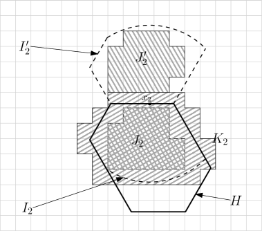
Figure 1: The hexagonal hull $H$ and regions $I_{2},J_{2},K_{2}$ and $I_{2}^{\prime},J_{2}^{\prime}$.

We consider the six tangents to the convex hull of $X$ making angles of $0$, $\frac{\pi}{3}$ and $\frac{2\pi}{3}$ with the $x$-axis (two for each angle). Together, these define a hexagon $H(X)$ containing $X$ whose edges are segments of the tangents (some of which may have zero length). We shall call $H(X)$ the hexagonal hull of $X$, and label its edges $E_{1},E_{2},\ldots E_{6}$ in cyclic order so that the top and bottom edges parallel to the $x$-axis are $E_{2}$ and $E_{5}$ respectively .

Consider $E_{1}$. There exists $x_{1}\in E_{1}\cap X$. Let $r_{1}$ be distance between $x_{1}$ and its $k$-th nearest neighbour. Let $I_{1}$ be the intersection of the ball of radius $r_{1}$ centred at $x_{1}$ with the hexagon $H(X)$. Let $I_{1}^{\prime}$ be the reflection of $I_{1}$ with respect to $L_{1}$. Since $I_{1}^{\prime}\subset U_{n}\setminus H(X)$ and since every point of $I_{1}^{\prime}$ lies at distance at most $r_{1}$ from $x_{1}$, it follows that $I_{1}^{\prime}$ contains no point of $\mathcal{P}$. We shall show that $I_{1}^{\prime}$ covers many tiles.

Let $J_{1}$ be the union of all of the tiles wholly contained inside $I_{1}$, and let $J_{1}^{\prime}$ be the union of all of the tiles wholly contained inside $I_{1}^{\prime}$. Let $K_{1}$ be the union of all of the tiles meeting $I_{1}$ and let $K_{1}^{\prime}$ be the union of all of the tiles meeting $I_{1}^{\prime}$. Since no tile in $U_{n}$ contains more than $(1+\eta)\frac{\log n}{N^{2}}$ points of $\mathcal{P}$, it follows that $K_{1}$ is the union of at least $\frac{k}{(1+\eta)\log n/N^{2}}$ tiles.

A tile is contained in $K_{1}\setminus J_{1}$ only if it meets the boundary of $I_{1}$. Now, since $I_{1}$ is a convex subset of a disc of radius $r_{1}$, the boundary of $I_{1}$ has length less than $2\pi r_{1}$, so by Lemma 10, $K_{1}\setminus J_{1}$ is the union of at most $\frac{18\pi r_{1}}{\sqrt{\log n}/N}$ tiles. By the same argument, $K_{1}^{\prime}\setminus J_{1}^{\prime}$ is the union of at most $\frac{18\pi r_{1}}{\sqrt{\log n}/N}$ tiles. Denote by $|I_{1}|$ the area of $I_{1}$, and similary $|I_{1}^{\prime}|,|J_{1}|,\ldots|K_{1}^{\prime}|$. We have

$$|J_{1}^{\prime}| \geq|I_{1}^{\prime}|-|K_{1}^{\prime}\setminus J_{1}^{\prime}|$$

$$\geq|I_{1}|-|K_{1}^{\prime}\setminus J_{1}^{\prime}|$$

$$\geq|K_{1}|-|K_{1}\setminus J_{1}|-|K_{1}^{\prime}\setminus J_{1}^{\prime}|.$$

Now each tile has area $\frac{\log n}{N^{2}}$. We therefore have

$$|J_{1}^{\prime}| \geq\frac{\log n}{N^{2}}\left(\frac{k}{(1+\eta)\log n/N^{2}}-\frac{36\pi r_{1}}{\sqrt{\log n}/N}\right)$$

$$\geq\frac{k}{1+\eta}-\frac{36\pi r_{1}\sqrt{\log n}}{N}$$

$$\geq\frac{k}{1+\eta}-\frac{9M\pi\log n}{2N}\qquad\textrm{since }r_{1}<\frac{M\sqrt{\log n}}{8}.$$

We turn at last to the choice of $N$: let $N=10\lceil 27M\pi\rceil$. For $k>0.3\log n$ and $\eta\leq\frac{1}{2}$, the above becomes:

$$|J_{1}^{\prime}| >\frac{11}{60}\log n.$$

For $i=2,3\ldots 6$ we may define $I_{i}$, $I_{i}^{\prime}$, etc… as above. It is easy to see that the $J_{i}^{\prime}$ are disjoint: each $J_{i}^{\prime}$ lies between the bisectors of two adjacent angles of the convex hexagon $H(X)$. Repeating the argument above to bound below $|J_{2}^{\prime}|$, $\ldots\ |J_{6}^{\prime}|$, we get:

$$\left|\bigcup_{i=1}^{6}J_{i}^{\prime}\right| =\sum_{i=1}^{6}|J_{i}^{\prime}|$$

$$>\frac{11}{10}\log n.$$

Thus there are at least $\frac{11}{10}\log n/(\log n/N^{2})=110{(\lceil 27M\pi\rceil)}^{2}$ tiles which receive no points. There are at most $\binom{M^{2}N^{2}}{110{(\lceil 27M\pi\rceil)}^{2}}$ ways of choosing this many tiles. Since $M$ and $N$ are constants this is just a (large) constant. The probability that there exist $110{(\lceil 27M\pi\rceil)}^{2}$ empty tiles (i.e., empty tiles with total area $\frac{11}{10}\log n$) in $U_{n}$ is therefore

$$O(\exp(-\frac{11}{10}\log n))=O(n^{-1.1}).$$

Thus

$$\mathbb{P}(A_{k}\setminus\bigcup_{Q}A_{k,Q})=O(n^{-1.1}),$$

as claimed.

∎

3 The sharp connectivity threshold for $S_{n,k}$

In Lemma 9 of the previous section we proved that small components witnessing $A_{k}$ have high point density. We use this fact to prove a sharpness result for $\mathbb{P}(A_{k})$, which by Corollary 8 implies in turn a sharp threshold for the connectivity of $S_{n,k}$ (i.e., Theorem 1). We shall do this by showing that, for all $k^{\prime}>k$, most pointsets in $A_{k^{\prime}}$ may be obtained by adding points to already dense parts of $A_{k}$ pointsets.

We shall need the following lemma, which is a convenient restatement of Theorem 5 of [1].

Lemma 11.

There exists a positive constant $c_{3}>0$ such that for every $\varepsilon$ with $0<\varepsilon\leq\frac{1}{2}$ and all $n>\varepsilon^{-c_{3}}$,

if $$k\leq 0.3\log n \mathbb{P}(S_{n,k}\textrm{ connected})<\varepsilon,$$, then

and if $$k\geq 0.6\log n \mathbb{P}(S_{n,k}\textrm{ connected})>1-\varepsilon.$$, then

Recall that in the previous section we fixed constants $0<\eta\leq\frac{1}{2}$ and $N\in\mathbb{N}$ and introduced a tiling of $U_{n}$ into $M^{2}N^{2}$ small square tiles as well as the families of events $A_{k,Q}$ and $A_{k,Q}^{\prime}$. Lemma 9 says that provided $\mathbb{P}(A_{k})=\Omega(n^{-1})$, we have $\mathbb{P}(\bigcup_{Q}A_{k,Q})=(1-O(n^{-0.1}))\mathbb{P}(A_{k})$. Thus if a small $A_{k}$ connected component occurs, then with high probability some tile $Q$ receives far more points than expected. We show that if $k^{\prime}>k$ then most $A_{k^{\prime}}$ pointsets can be obtained by adding points to an overpopulated tile of an $A_{k}$ pointset.

We need one more piece of notation: given a tile $Q$ let $A_{k,Q,L}$ be the event that if we remove any $L$ points from $Q$ then $A_{k,Q}^{\prime}$ occurs.

Lemma 12.

For any tile $Q$ and positive integer $L<\frac{\eta\log n}{2N^{2}}$ we have

$$A_{k+L,Q}\subseteq A_{k,Q,L}.$$

Proof.

Suppose that $\mathcal{P}\subset U_{n}$ is a pointset for which the event $A_{k+L,Q}$ occurs. It is enough to show that the removal of any $L$ points from $\mathcal{P}\cap Q$ yields a pointset $\mathcal{P}^{\prime}$ for which the event $A_{k,Q}^{\prime}$ occurs.

As in Lemma 9, write $U_{n,k}(\mathcal{P})$ for the $k$ nearest neighbours graph on $U_{n}$ associated with the pointset $\mathcal{P}$. Since we remove at most $L$ vertices from $\mathcal{P}$ every vertex in $\mathcal{P}$ loses at most $L$ of its $k+L$ nearest neighbours; the set of its $k$ nearest neighbours in $\mathcal{P}^{\prime}$ is thus a subset of the set of its $k+L$ nearest neighbours in $\mathcal{P}$. It follows that $U_{n,k}(\mathcal{P}^{\prime})$ is a subgraph of $U_{n,k+L}(\mathcal{P})$.

$U_{n,k+L}(\mathcal{P})$ has a connected component wholly contained inside $\frac{1}{2}U_{n}$. This component must contain at least $k+L+1>L$ vertices and since we have removed only $L$ vertices from $\mathcal{P}$ to obtain $\mathcal{P}^{\prime}$ some vertices of this component remain: that is, $U_{n,k}(\mathcal{P}^{\prime})$ must also have component wholly contained inside $\frac{1}{2}U_{n}$. Thus $\mathcal{P}^{\prime}\in A_{k}$.

Moreover the number of points in $\mathcal{P}^{\prime}\cap Q$ is exactly

$$|\mathcal{P}\cap Q|-L >(1+\eta)\frac{\log n}{N^{2}}-\frac{\eta\log n}{2N^{2}}=(1+\frac{\eta}{2})\frac{\log n}{N^{2}}$$

and hence $\mathcal{P}^{\prime}\in A_{k,Q}^{\prime}$ as claimed. ∎

Corollary 13.

Let $L<\frac{\eta\log n}{2N^{2}}$ be a positive integer and $Q$ a tile. Then

$$\mathbb{P}(A_{k+L,Q})<(1+\frac{\eta}{2})^{-L}\mathbb{P}(A_{k,Q}^{\prime}).$$

Proof.

First, note that we may consider the Poisson process on $U_{n}$ as the union of a Poisson process on $Q$ and an independent Poisson process on the disjoint set $U_{n}\setminus Q$. Now a Poisson point process on $Q$ is just a uniform point process placing

$$Z\sim~{}\textrm{Poisson}\left(\frac{\log n}{N^{2}}\right)$$

points in $Q$.

We may think of this uniform point process as adding points one by one. If $A_{k,Q,L}$ occurs then in particular $A_{k,Q}^{\prime}$ occurs if we remove the last $L$ points added by the point process. It follows that

$$\mathbb{P}(A_{k+L,Q}) \leq\mathbb{P}(A_{k,Q,L})$$ by Lemma 12

$$=\sum_{m}\mathbb{P}(A_{k,Q,L}|Z=m+L)\mathbb{P}(Z=m+L)$$

$$\leq\sum_{m}\mathbb{P}(A_{k,Q}^{\prime}|Z=m)\mathbb{P}(Z=m+L) A_{k,Q,L}$$ by definition of

$$=\sum_{m}\mathbb{P}(A_{k,Q}^{\prime}|Z=m)\mathbb{P}(Z=m)\prod_{i=1}^{L}\frac{N^{-2}\log n}{m+i}$$

By the definition of $A_{k,Q}^{\prime}$,

$$\mathbb{P}(A_{k,Q}^{\prime}|Z=m)=0\qquad\textrm{ for all }m<(1+\frac{\eta}{2})\frac{\log n}{N^{2}}.$$

For $m\geq(1+\frac{\eta}{2})\frac{\log n}{N^{2}}$, we have

$$\prod_{i=1}^{L}\frac{N^{-2}\log n}{m+i}<\left(\frac{N^{-2}\log n}{m}\right)^{L}\leq{(1+\frac{\eta}{2})}^{-L}.$$

It follows that

$$\mathbb{P}(A_{k+L,Q})<{(1+\frac{\eta}{2})}^{-L}\mathbb{P}(A_{k,Q}^{\prime}),$$

as claimed. ∎

Theorem 14.

There are constants $c_{4}$ and $L\in\mathbb{N}$ such that for all $n>c_{4}$ and all $k$ with

$$k\in[0.3\log n,0.6\log n]\textrm{ and }\mathbb{P}(A_{k})\geq n^{-1.05}$$

we have:

$$\mathbb{P}(A_{k+L})<e^{-1}\,\mathbb{P}(A_{k}).$$

Proof.

Let $L$ be an integer constant which we shall specify later on. As $\eta$, $L$ and $N$ are all constants, for an appropriate choice of our constant $c_{4}>0$ and all $n>c_{4}$, we have $L<\frac{\eta\log n}{2N^{2}}$ so that the hypothesis of Corollary 13 is satisfied. Also $k\in[0.3\log n,0.6\log n]$, so the hypothesis of Lemma 9 is satisfied as well. Applying the two lemmas successively, we get:

$$\mathbb{P}(A_{k+L}) =\mathbb{P}(\bigcup_{Q}A_{k+L,Q})+O(n^{-1.1})\qquad$$ by Lemma 9

$$\leq\sum_{Q}\mathbb{P}(A_{k+L,Q})+O(n^{-1.1})$$

$$\leq\sum_{Q}(1+\frac{\eta}{2})^{-L}\mathbb{P}(A_{k,Q}^{\prime})+O(n^{-1.1})$$ by Corollary 13

$$\leq M^{2}N^{2}(1+\frac{\eta}{2})^{-L}\mathbb{P}(A_{k})+O(n^{-1.1}) \mathbb{P}(A_{k,Q}^{\prime})\leq\mathbb{P}(A_{k})$$ (since .)

We now choose $L$: let

$$L=\left\lceil\frac{\log\left(M^{2}N^{2}e^{2}\right)}{\log(1+\frac{\eta}{2})}\right\rceil$$

so that

$$M^{2}N^{2}(1+\frac{\eta}{2})^{-L}\leq e^{-2}.$$

By assumption $\mathbb{P}(A_{k})\geq n^{-1.05}$, so for an appropriate choice of our constant $c_{4}>0$ and all $n>c_{4}$, we have

$$\mathbb{P}(A_{k+L})<e^{-1}\,\mathbb{P}(A_{k}),$$

as claimed. (Note that the choice of our constant $L$ depended only on the constant $M$, $N$ and $\eta$.) ∎

Proof of Theorem 1.

In essence, we just iterate Theorem 14. However, we have to choose the right parameters and make sure the conditions hold at each stage.

We choose $\gamma>0$ such that $\gamma>\max\left(c_{2},c_{3},\log_{2}c_{4},20\right)$. Note that, since $M\geq 30$, we have $\frac{e^{4}}{M^{2}\log n}\leq\frac{e^{4}}{900\log 2}<0.09$ for all $n\geq 2$ so $n^{-1/\gamma}>\frac{e^{4}}{M^{2}\log n}n^{-0.05}$ for all $n\geq 2$.

Suppose that $n$ and $k$ are such that $\mathbb{P}(S_{n,k}\textrm{ is connected})>\varepsilon$ and $n>\varepsilon^{-\gamma}$. We may assume that $\varepsilon\leq\frac{1}{2}$ and $\mathbb{P}(S_{n,k}\textrm{ connected})\leq 1-\varepsilon$, for otherwise we have nothing to prove. Since $n>\varepsilon^{-\gamma}>\varepsilon^{-c_{3}}$ and $\varepsilon<\mathbb{P}(S_{n,k}\textrm{ connected})<1-\varepsilon$, Lemma 11 implies that $0.3\log n<k<0.6\log n$. Thus, for $n>\varepsilon^{-\gamma}$, the assumptions of Corollary 8 and Theorem 14 are therefore satisfied.

Let $C$ be a strictly positive real constant which we shall specify later on. There are three cases to consider.

Suppose first of all that

$$k+\lfloor C\log\frac{1}{\varepsilon}\rfloor\geq 0.6\log n.$$

Then by Lemma 11 we have $\mathbb{P}(S_{n,k+\lfloor C\log(1/\varepsilon)\rfloor}\textrm{ connected})>1-\varepsilon$, and we are done.

Secondly suppose that $k+\lfloor C\log\frac{1}{\varepsilon}\rfloor<0.6\log n$ and

$$\mathbb{P}(A_{k+\lfloor C\log(1/\varepsilon)\rfloor})<n^{-1.05}.$$

Since $n>\varepsilon^{-\gamma}$,

$$n^{-1.05}<n^{-1/\gamma}\frac{M^{2}\log n}{e^{4}n}<\varepsilon\frac{M^{2}\log n}{e^{4}n},$$

so that by Corollary 8 we have $\mathbb{P}(S_{n,k+\lfloor C\log(1/\varepsilon)\rfloor}\textrm{ connected})>1-\varepsilon$, and we are done.

Finally if

$$k+\lfloor C\log\frac{1}{\varepsilon}\rfloor<0.6\log n\qquad\textrm{and}\qquad\mathbb{P}(A_{k+\lfloor C\log(1/\varepsilon)\rfloor})\geq n^{-1.05},$$

then since $\mathbb{P}(A_{k^{\prime}})$ monotonically decreases as $k^{\prime}$ increases we have $\mathbb{P}(A_{k^{\prime}})\geq n^{-1.05}$ for every $k^{\prime}:k\leq k^{\prime}\leq k+\lfloor C\log\frac{1}{\varepsilon}\rfloor$. Thus by Theorem 14 we have, for all $k^{\prime}:k\leq k^{\prime}\leq k+\lfloor C\log\frac{1}{\varepsilon}\rfloor$,

$$\mathbb{P}(A_{k^{\prime}+L})<e^{-1}\mathbb{P}(A_{k^{\prime}}).$$

Since $k<0.6\log n$, $\mathbb{P}(S_{n,k}\textrm{ connected})\leq 1-\varepsilon$ implies by Corollary 8 that $\mathbb{P}(A_{k})\leq\frac{eM^{2}\log n}{n}\log\frac{1}{\varepsilon}$. Thus

$$\mathbb{P}(A_{k+\lfloor C\log\frac{1}{\varepsilon}\rfloor}) \leq\exp\left(-\left\lfloor\frac{\lfloor C\log 1/\varepsilon\rfloor}{L}\right\rfloor\right)\mathbb{P}(A_{k})$$

$$\leq\exp\left(-\left\lfloor\frac{C\log 1/\varepsilon}{L}\right\rfloor\right)\left(\frac{eM^{2}\log n}{n}\log\frac{1}{\varepsilon}\right)$$

$$\leq\exp\left(-\left\lfloor\frac{C\log 1/\varepsilon}{L}\right\rfloor+1+\log\log{1}/{\varepsilon}\right)\frac{M^{2}\log n}{n}.$$

We now choose $C$: let

$$C=\left(2+\frac{6}{\log 2}\right)L.$$

Since $\varepsilon\leq\frac{1}{2}$, we have that $\frac{\log 1/\varepsilon}{\log 2}\geq 1$. Thus for this choice of $C$ we have

$$-\left\lfloor\frac{C\log 1/\varepsilon}{L}\right\rfloor +1+\log\log\frac{1}{\varepsilon}$$

$$\leq 2+\log\log\frac{1}{\varepsilon}-\frac{C\log 1/\varepsilon}{L}$$

$$=(2-2\frac{\log 1/\varepsilon}{\log 2})+(\log\log\frac{1}{\varepsilon}-\log\frac{1}{\varepsilon})-\frac{4\log 1/\varepsilon}{\log 2}-\log\frac{1}{\varepsilon}$$

$$\leq-4-\log\frac{1}{\varepsilon}.$$

Substituting this in the above bound for $\mathbb{P}(A_{k+\lfloor C\log{1}/{\varepsilon}\rfloor})$ we get

$$\mathbb{P}(A_{k+\lfloor C\log 1/\varepsilon\rfloor})\leq\varepsilon\frac{M^{2}\log n}{e^{4}n}.$$

By Corollary 8 this implies

$$\mathbb{P}(S_{n,k+\lfloor C\log{1}/{\varepsilon}\rfloor}\textrm{ connected})>1-\varepsilon,$$

proving the theorem. ∎

4 Higher connectivity

In this section, we shall apply our sharpness result Theorem 1 to prove Theorem 2, proving a conjecture of Balister, Bollobás, Sarkar and Walters [3]. Suppose that ${\mathcal{P}}$ is any pointset in in the square $S_{n}=[0,\sqrt{n}]^{2}$. As before, let $G_{k}({\mathcal{P}})$ denote the $k$ nearest neighbour graph on ${\mathcal{P}}$.

Lemma 15.

Suppose $S_{n,k}$ is the random geometric graph with $k$ an integer lying between $0.3\log n$ and $0.6\log n$. Let $s<0.1\log n$. Then there is a constant $c_{6}$ such that

$$\mathbb{P}(S_{n,k}\text{ not $s$-connected})\leq c_{6}(\log n)\mathbb{P}(S_{n,k-1}\text{ not $(s-1)$-connected})+O(n^{-3}).$$

Moreover

$$\mathbb{P}(S_{n,k}\text{ not $s$-connected})\leq(c_{6}\log n)^{s-1}\mathbb{P}(S_{n,k-s+1}\text{ not connected})+O\left(n^{-3}\log n\right).$$

We shall need the following technical result to prove Lemma 15.

Lemma 16.

Suppose $0.3\log n<k<0.6\log n$. Then there exists $c_{7}$ such that the collection of pointsets ${\mathcal{P}}$ from which we may delete at set $T$ of at most $0.1\log n$ points so that either of the following hold:

• there is any point $x\in S_{n}$ (not necessarily in ${\mathcal{P}}$) with $\lceil 0.6\log n\rceil$-nearest neighbour radius in $\mathcal{P}\setminus S$ at least $c_{7}\sqrt{\log n}$

• $G_{k}({\mathcal{P}})\setminus T$ contains at least two components of diameter at least $c_{7}\sqrt{\log n}$

has probability $O(n^{-3})$.

Proof.

This is an easy modification of Lemmas 2 and 6 of [1] ∎

Proof of Theorem 15.

We can view the Poisson distribution as follows. Suppose that $X_{1},X_{2},X_{3},\ldots$ is an infinite sequence of uniformly distributed random variables in $S_{n}$ and let $Z\sim{\rm Po}(n)$. Then let the points in ${\mathcal{P}}$ be given by $(X_{i})_{i=1}^{Z}$. Let ${\mathcal{P}}_{m}$ denote the collection of pointsets with exactly $m$ points which we give the conditional measure which we shall sometimes denote $\mathbb{P}_{m}$. From this point of view it is easy to see that we have $m$ measure preserving maps $\phi_{i}$ for $1\leq i\leq m$ from ${\mathcal{P}}_{m}$ to ${\mathcal{P}}_{m-1}$ given by deleting the point $X_{i}$. We shall usually abbreviate $\phi_{1}$ to $\phi$.

Let ${\mathcal{A}}_{s}$ denote the collection of pointsets ${\mathcal{P}}$ for which $G_{k}({\mathcal{P}})$ is not $s$-connected but $G_{k-1}({\mathcal{P}})$ is $(s-1)$-connected. Let ${\mathcal{B}}_{s}$ denote those pointsets ${\mathcal{P}}$ for which $G_{k-1}({\mathcal{P}})$ is not $(s-1)$-connected. Finally let ${\mathcal{C}}$ denote the collection of pointsets ${\mathcal{P}}$ for which either of the conditions in Lemma 16 hold, which we shall think of as the ‘bad’ pointsets. By Lemma 16, $\mathbb{P}({\mathcal{C}})=O(n^{-3})$.

For any pointset ${\mathcal{P}}$ in ${\mathcal{A}}_{s}$ it is clear that (at least) one of the functions $\phi_{i}$ maps ${\mathcal{P}}$ into ${\mathcal{B}}_{s}$. Indeed, since $G_{k}({\mathcal{P}})$ is not $s$-connected, there is a point $X_{i}$ which we can delete to make the graph not $(s-1)$-connected. Since $G_{k-1}({\mathcal{P}}\setminus X_{i})$ is a subgraph of $G_{k}({\mathcal{P}})\setminus X_{i}$ the map $\phi_{i}$ is one such function. Thus ${\mathcal{A}}_{s}\subseteq\bigcup_{i=1}^{m}\phi_{i}^{-1}({\mathcal{B}}_{s})$.

Note that $\mathbb{P}(|Z-n|>n/2)=o(e^{-n/2})$. We have

$$\mathbb{P}({\mathcal{A}}_{s}) =\sum_{m=0}^{\infty}\mathbb{P}({\mathcal{A}}_{s}|Z=m)\mathbb{P}(Z=m)$$

$$=\sum_{m=n/2}^{3n/2}\mathbb{P}({\mathcal{A}}_{s}|Z=m)\mathbb{P}(Z=m)+o(e^{-n/2})$$

$$=\sum_{m=n/2}^{3n/2}\mathbb{P}_{m}({\mathcal{A}}_{s}\setminus{\mathcal{C}})\mathbb{P}(Z=m)+O(n^{-3})$$

$$=\sum_{m=n/2}^{3n/2}\mathbb{P}_{m}({\mathcal{P}}\in{\mathcal{A}}_{s}\setminus{\mathcal{C}}\text{ and }\exists i:\phi_{i}({\mathcal{P}})\in{\mathcal{B}}_{s})\mathbb{P}(Z=m)+O(n^{-3})$$

$$\leq\sum_{m=n/2}^{3n/2}\sum_{i=1}^{m}\mathbb{P}_{m}({\mathcal{P}}\in{\mathcal{A}}_{s}\setminus{\mathcal{C}}\text{ and }\phi_{i}({\mathcal{P}})\in{\mathcal{B}}_{s})\mathbb{P}(Z=m)+O(n^{-3})$$

$$=\sum_{m=n/2}^{3n/2}m\mathbb{P}_{m}({\mathcal{P}}\in{\mathcal{A}}_{s}\setminus{\mathcal{C}}\text{ and }\phi({\mathcal{P}})\in{\mathcal{B}}_{s})\mathbb{P}(Z=m)+O(n^{-3}).$$

Now consider $\mathbb{P}_{m}({\mathcal{P}}\in{\mathcal{A}}_{s}\setminus{\mathcal{C}}\text{ and }\phi({\mathcal{P}})\in{\mathcal{B}}_{s})$. For each ${\mathcal{P}}\in{\mathcal{A}}_{s}\setminus{\mathcal{C}}$ with $\phi({\mathcal{P}})\in{\mathcal{B}}_{s}$ we see that $G_{k-1}({\mathcal{P}})$ is $(s-1)$-connected but $G_{k-1}(\phi({\mathcal{P}}))$ is not $(s-1)$-connected. Fix a separating set $T$ of $s-1$ vertices for $G_{k-1}(\phi({\mathcal{P}}))$. Since ${\mathcal{P}}\notin{\mathcal{C}}$ we have that all but one of the components in the separated graph $G_{k-1}(\phi({\mathcal{P}}))\setminus T$ are small: less than $c_{7}\sqrt{\log n}$ in diameter. Fix one such component $C$. Since $G_{k-1}({\mathcal{P}})$ is $(s-1)$-connected we see that $G_{k-1}({\mathcal{P}})\setminus T$ is connected so $X_{1}$ must be joined to $C$ in $G_{k-1}({\mathcal{P}})$ and, hence, that $X_{1}$ lies within distance $c_{7}\sqrt{\log n}$ of $C$. Therefore $X_{1}$ lies within a set of measure less than $4\pi c_{7}^{2}\log n$ which is determined by ${\mathcal{P}}\setminus X_{1}$. This event has probability less than $\left(\frac{4\pi c_{7}^{2}\log n}{n}\right)$. Thus, as $\phi$ is a measure preserving transformation from $\mathbb{P}_{m}$ to $\mathbb{P}_{m-1}$,

$$\mathbb{P}_{m}({\mathcal{P}}\in{\mathcal{A}}_{s}\setminus{\mathcal{C}}\text{ and }\phi({\mathcal{P}})\in{\mathcal{B}}_{s}) \leq\left(\frac{4\pi c_{7}^{2}\log n}{n}\right)\mathbb{P}_{m}(\phi({\mathcal{P}})\in{\mathcal{B}}_{s})$$

$$=\left(\frac{4\pi c_{7}^{2}\log n}{n}\right)\mathbb{P}_{m-1}({\mathcal{P}}\in{\mathcal{B}}_{s})$$

To complete the proof note that $\mathbb{P}(Z=m)\leq 2\mathbb{P}(Z=m-1)$ for all $m>n/2$. Thus

$$\mathbb{P}(A_{s}) \leq\sum_{m=n/2}^{3n/2}m\mathbb{P}_{m}({\mathcal{P}}\in{\mathcal{A}}_{s}\setminus{\mathcal{C}}\text{ and }\phi({\mathcal{P}})\in{\mathcal{B}}_{s})\mathbb{P}(Z=m)+O(n^{-3})$$

$$\leq\sum_{m=n/2}^{3n/2}m\left(\frac{4\pi c_{7}^{2}\log n}{n}\right)\mathbb{P}_{m-1}({\mathcal{P}}\in{\mathcal{B}}_{s})\mathbb{P}(Z=m)+O(n^{-3})$$

$$\leq\sum_{m=n/2}^{3n/2}\left(12\pi c_{7}^{2}\log n\right)\mathbb{P}_{m-1}({\mathcal{P}}\in{\mathcal{B}}_{s})\mathbb{P}(Z=m-1)+O(n^{-3})$$

$$\leq\left(12\pi c_{7}^{2}\log n\right)\mathbb{P}({\mathcal{B}}_{s})+O(n^{-3}).$$

Finally observe that

$$\{{\mathcal{P}}\ :\ S_{n,k}\text{ not $s$-connected}\}\subseteq{\mathcal{A}}_{s}\cup{\mathcal{B}}_{s}$$

so that the first part of the lemma holds with $c_{6}=12\pi c_{7}^{2}+1$:

$$\mathbb{P}(S_{n,k}\textrm{ not $s$-connected})\leq c_{6}\log n\mathbb{P}(S_{n,k-1}\textrm{ not $(s-1)$-connected})+O(n^{-3}).$$

Iterating this $s-1=O(\log n)$ times we obtain the second part of our claim. ∎

We can now finally turn to the proof of Theorem 2.

Proof of Theorem 2.

By Theorem 2 of [3] we may restrict ourselves to the case where $s(n)$ is an integer sequence with $s(n)\leq\frac{\log n}{2\gamma\log\log n}$. Suppose that $k=k(n)$ is such that $S_{n,k}$ is connected whp, so that

$$\mathbb{P}(S_{n,k}\text{ is not connected})\to 0.$$

By Theorem 1 with $\varepsilon={(c_{6}\log n)}^{-s}$,

$$\mathbb{P}(S_{n,k+\lfloor C\log 1/\varepsilon\rfloor}\text{ is not connected})<\varepsilon$$

for all sufficiently large $n$. (Explicitly, this is for all $n$ with $n>\varepsilon^{-\gamma}$. Given our choice of $\varepsilon$ and the restriction on $s$, $\varepsilon^{-\gamma}$ is at most $\exp(\frac{1}{2}\log n+O(\frac{\log n}{\log\log n}))$, so that this is indeed satisfiable for large enough $n$.) Now

$$C\log\frac{1}{\varepsilon}+s-1 <2Cs\log\log n$$

for all sufficiently large $n$. If $k+\lfloor 2Cs\log\log n\rfloor<0.6\log n$, we have by Lemma 15

$$\mathbb{P}( S_{n,k+\lfloor 2Cs\log\log n\rfloor}\text{ not $s$-connected})$$

$$\leq{(c_{6}\log n)}^{s-1}\mathbb{P}(S_{n,k-s+1+\lfloor 2Cs\log\log n\rfloor}\textrm{ not connected})+O\left(n^{-3}\log n\right)$$

$$\leq{(c_{6}\log n)}^{s-1}\mathbb{P}(S_{n,k+\lfloor C\log 1/\varepsilon\rfloor}\textrm{ not connected})+O\left(n^{-3}\log n\right)$$

$$<(c_{6}\log n)^{s-1}\varepsilon+O\left(n^{-3}\log n\right)$$

$$=O(1/\log n)=o(1)$$

as required. If on the other hand $k+\lfloor 2Cs\log\log n\rfloor\geq 0.6\log n$, we have

$$\mathbb{P}(S_{n,k+\lfloor 2Cs\log\log n\rfloor}\text{ is not $s$-connected})=o(1)$$

by Theorem 2 of [3]. The result follows. ∎