Stochastic quantum molecular dynamics for finite and extended systems

Abstract

We present a detailed account of the technical aspects of stochastic quantum molecular dynamics, an approach introduced recently by the authors [H. Appel and M. Di Ventra, Phys. Rev. B 80 212303 (2009)] to describe coupled electron-ion dynamics in open quantum systems. As example applications of the method we consider both finite systems with and without ionic motion, as well as describe its applicability to extended systems in the limit of classical ions. The latter formulation allows the study of important phenomena such as decoherence and energy relaxation in bulk systems and surfaces in the presence of time-dependent fields.

1 Introduction

Time-dependent density-functional theory (TDDFT) calculations are currently enjoying a large popularity due to their efficiency and success in describing low-lying excitation energies in molecular systems [1]. In addition, many applications have been investigated with TDDFT. Examples include electronic transport [2, 3, 4, 5], nonlinear optical response [6], or atoms and molecules in strong laser fields [7, 8]. In the latter cases, the time-dependent Kohn-Sham (TDKS) equations are usually evolved in real-time. However, the majority of these studies pertains to the description of closed quantum systems, since the corresponding TDKS equations describe a set of N particles evolving coherently in time.  On the other hand, most experimental situations involve some level of energy dissipation and/or decoherence induced by either some environments to which the given system is coupled, or the measurement apparatus itself which necessarily projects non-unitarily the state of the system onto states of the observables. This is generally true for both electrons and ions, so that a first-principles description of their coupled dynamics in the presence of one or more environments is of fundamental importance in order to describe phenomena and compare with experiments. At this point, it is worth noting that present quantum molecular dynamics (QMD) approaches, (e.g., the Born-Oppenheimer, Ehrenfest or Car-Parrinello methods) either do not allow excited states dynamics (Born-Oppenheimer and Car-Parrinello methods) or, if they do (e.g., Ehrenfest QMD), they do not permit electronic coupling to external environments. Indeed, in all these approaches, energy dissipation and thermal coupling to the environment are usually described with additional thermostats coupled directly to the classical nuclear degrees of freedom, which fall short of describing the numerous physical phenomena associated with decoherence and energy dissipation.

In order to overcome these shortcomings, we have recently introduced a novel time-dependent density functional approach based on stochastic time-dependent Kohn-Sham equations [13], where we allow the coupling of both electrons and (in principle quantum) ions with external baths. This approach - we have named stochastic quantum molecular dynamics (SQMD) - extends the previously introduced stochastic time-dependent-current density-functional theory (STDCDFT) [9, 10] to the coupled dynamics of electrons and ions. The latter was formulated to account for electrons interacting with external environments, without however including atomic motion. Therefore, SQMD combines and improves on the strengths of STDCDFT and present QMD methods by greatly expanding the physical range of applications of these methods.

Clearly, from a practical point of view the present approach suffers - like all density-functional theory (DFT) based methods - from our limited knowledge of the properties of the exact exchange-correlation functional. Furthermore, in the present case, the exact functional depends not only on the electronic degrees of freedom, but also on the ionic and bath(s) degrees of freedom [13]. Nevertheless, due to the weak system-bath(s) coupling assumption of the present theory, as well as the limited number of systems where quantum nuclear effects are of disproportionate importance, we may start by considering the limit of SQMD to classical nuclei and adopt the available functionals of standard closed-system TDDFT. Like in any other practical application of DFT, it is the predictions that we obtain and comparison with experiments that will be the ultimate judge of the range of validity of the approximate functionals used.

In Ref. [13] we have outlined the details of the proof of the theorem at the core of SQMD, and provided a simple example of the relaxation dynamics of a finite system (a molecule) prepared in some excited state and embedded in a thermal bath. However, there are some technical details behind an actual implementation of this approach we have not reported yet, and which are nonetheless important if one is interested in using this method for practical computations. In this work we then present all the technical aspects for a practical implementation and use of SQMD. In addition, we present the theory behind its applicability to extended systems which is of great importance in the study of decoherence and energy relaxation in bulk systems and surfaces. We are in the process of implementing SQMD for extended systems and we will report these results in a forthcoming publication [14].

The paper is organized as follows. In Section 2 we give an introduction to the theory of stochastic quantum molecular dynamics. For completeness, this includes general aspects of open quantum systems as well as the basic theorem of SQMD. In Section 3 we discuss the aspects of a practical implementation of SQMD. Finally, in Section 4 we illustrate with some examples the application of SQMD to finite systems with and without ionic motion, and outline its extension to periodic systems. Conclusions are reported in Section 5.

2 Theory

2.1 Stochastic Schrödinger equation

In the following, we consider an electron-ion many-body system coupled to a bosonic bath. For simplicity, we will consider only a single bath, but the formulation is trivially extended to the case of several environments. The total Hamiltonian of the entire system is then

$$\hat{H}=\hat{H}_{S}\otimes\hat{I}_{B}+\hat{I}_{S}\otimes\hat{H}_{B}+\lambda\hat{H}_{SB}.$$ (1)

Our system of interest is described by the many-body Hamiltonian $\hat{H}_{S}$ and the environment degrees of freedom are given in terms of $\hat{H}_{B}$. The interaction of the system with the environment is given by the Hamiltonian $\hat{H}_{SB}$ and is assumed to be weak in the sense that a perturbation expansion in terms of this coupling can be performed. With $\lambda$ we denote the corresponding coupling parameter for the system-bath interaction.

The total system described by the Hamiltonian $\hat{H}$ follows a unitary time-evolution, which can be formulated for pure states either in terms of the time-dependent Schrödinger equation (TDSE), with $\hbar=1$

$$i\partial_{t}\Psi(t)=\hat{H}(t)\Psi(t),$$ (2)

or, alternatively for mixed states, in terms of the Liouville-von Neumann equation

$$\frac{d}{dt}\hat{\rho}(t)=-i\left[\hat{H}(t),\hat{\rho}(t)\right],$$ (3)

where $\hat{\rho}$ is the statistical operator.

Since $\hat{H}$ is a many-body Hamiltonian and we have to deal, in principle, with infinitely many degrees of freedom (due to the bath) it is not possible to solve Eq. (2) or (3) in practice, except for a few simple model cases. In addition, in most cases of interest the microscopic knowledge about the bath is limited and only its macroscopic thermodynamic properties are known, e.g., one typically assumes that the bath is in thermal equilibrium. However, we are only interested in the dynamics of the system degrees of freedom. It is therefore desirable to find an effective description for the system only.

To accomplish this we may trace out the bath degrees of freedom at the level of the statistical operator, namely we perform the operation $\hat{\rho}_{S}=\textrm{Tr}_{B}\{\hat{\rho}\}$, where $\hat{\rho}_{S}$ is called the reduced statistical operator of system $S$. It is worth pointing out here that this procedure does not generally lead to a closed equation of motion for the reduced statistical operator and one needs further approximations. Depending on the approximations involved, one may arrive at an effective quantum master equation for the reduced density operator $\hat{\rho}_{S}$ [15, 16, 17]. As we will discuss later, this approach has some drawbacks when used within a density-functional formulation, both fundamental - in view of the theorems of DFT - and practical, since solving for the density matrix is computationally more demanding than solving directly for state vectors.

We therefore take here a different route. Instead of working with a derived/composite quantity like the statistical operator, we summarize briefly how the bath degrees of freedom can be traced out directly at the level of the wavefunction. The derivation that follows has been reported elsewhere in the literature (see, e.g., Ref. [18]). We repeat some steps here for completeness and to clarify our starting point.

To this end let us consider the set of eigenfunctions $\{\chi_{n}(x_{B})\}$ of the bath Hamiltonian

$$\hat{H}_{B}\chi_{n}(x_{B})=\varepsilon_{n}\chi_{n}(x_{B}),$$ (4)

with $x_{B}$ the bath’s coordinates (including possibly spin), and expand the total wavefunction of Eq. (2) in the complete set of orthonormal states formed by $\{\chi_{n}(x_{B})\}$, namely 

$$\Psi(x_{S},x_{B};t)=\sum_{n}\phi_{n}(x_{S};t)\chi_{n}(x_{B}),$$ (5)

with $\phi_{n}(x_{S};t)$ some functions (not necessarily normalized) in the Hilbert space of the system $S$.

In order to see that in the presence of a bath the functions $\phi_{n}(x_{S};t)$ form a statistical ensemble describing the properties of the subsystem $S$, let us proceed as follows. For a general observable $\hat{O}_{S}$ of the system $S$ we find after simple algebra (and using the orthonormality of the bath states $\chi_{n}(x_{B})$)

$$\begin{split}\langle\Psi(x_{S},x_{B};t)|\hat{O}_{S}&|\Psi(x_{S},x_{B};t)\rangle=\\ &\sum_{n}\langle\phi_{n}(x_{S};t)|\hat{O}_{S}|\phi_{n}(x_{S};t)\rangle.\end{split}$$ (6)

Let us now normalize the functions $\phi_{n}(x_{S};t)$ by writing

$$\psi_{n}(x_{S},t)\equiv\phi_{n}(x_{S};t)/p_{n}(t)$$ (7)

with

$$p_{n}(t)=\langle\phi_{n}(x_{S};t)|\phi_{n}(x_{S};t)\rangle,$$ (8)

which, according to Eq. (5), is nothing other than the probability for the bath to be in the state $\chi_{n}(x_{B})$.

We can now define the following statistical operator

$$\begin{split}\hat{\rho}_{S}&\equiv\sum p_{n}(t)|\psi_{n}(x_{S};t)\rangle\langle\psi_{n}(x_{S};t)|\\ &\equiv\overline{|\psi(t)\rangle\langle\psi(t)|},\end{split}$$ (9)

and immediately recognize that the average (6) can be re-written as

$$\langle\Psi(x_{S},x_{B};t)|\hat{O}_{S}|\Psi(x_{S},x_{B};t)\rangle=\textrm{Tr}\{\hat{\rho}_{S}O_{S}\},$$ (10)

namely, due to the interaction with the bath, the system $S$ is necessarily in a mixture of states defined by the macrostate $\{p_{n}(t),\psi_{n}(x_{S};t)\}$. We thus expect that the equation of motion for the representative wave-function $\psi(t)$ of the subsystem $S$ to be “naturally” stochastic, namely we expect to find an equation of motion that provides the macrostate $\{p_{n}(t),\psi_{n}(x_{S};t)\}$.

In order to show this we follow the Feshbach projection-operator method [19, 20] and define the following projection operators

$$\hat{P}_{n} :=\hat{I}_{S}\otimes\,|\,\chi_{n}{\,\rangle}{\langle\,}\chi_{n}\,|\,,$$ (11)

$$\hat{Q}_{n} :=\hat{I}_{S}\otimes\sum_{k\neq n}\,|\,\chi_{k}{\,\rangle}{\langle\,}\chi_{k}\,|\,,$$ (12)

where $\hat{I}_{S}$ is the identity in the Hilbert space of the system. The rationale behind the choice of the above operators is to obtain the equation of motion of a representative coefficient $\phi_{n}(x_{S};t)$.

By acting with these projection operators on the many-body TDSE for the combined system and bath in Eq. (2) we arrive at

$$i\partial_{t}\hat{P}_{n}\Psi(t)=\hat{P}_{n}\hat{H}\hat{P}_{n}\Psi(t)+\hat{P}_{n}\hat{H}\hat{Q}_{n}\Psi(t)$$ (13)

$$i\partial_{t}\hat{Q}_{n}\Psi(t)=\hat{Q}_{n}\hat{H}\hat{Q}_{n}\Psi(t)+\hat{Q}_{n}\hat{H}\hat{P}_{n}\Psi(t)$$ (14)

Equation (14) can be formally solved. Inserting the result back into Eq. (13) we obtain

$$\begin{split}i\partial_{t}&\hat{P}\Psi(t)=\hat{P}\hat{H}\hat{P}\hat{P}\Psi(t)+\hat{P}\hat{H}\hat{Q}e^{-i\hat{Q}\hat{H}\hat{Q}t}\hat{Q}\Psi(0)\\ &-i\int_{0}^{t}\,\hat{P}\hat{H}\hat{Q}e^{i\hat{Q}\hat{H}\hat{Q}(\tau-t)}\hat{Q}\hat{H}\hat{P}\hat{P}\Psi(\tau)\,d\tau,\end{split}$$ (15)

where we have omitted the index $n$ for brevity. The first term on the right hand side of Eq. (15) contains only projections on the system manifold, and describes the coherent evolution of the system degrees of freedom. The second term is a source term that carries a dependence on initial conditions ($\hat{Q}\Psi(0)$ are the initial conditions of all system’s states except the one we are considering), and the third term on the right hand side is a memory term that is recording the history of the time evolution.

Note that, up to this point, we have made no approximations, i.e., the time evolution given by Eq. (15) is still fully coherent. However, the solution of Eq. (15) is very involved and, apart from model systems, not feasible in practice. Furthermore, a solution would require the initial conditions for all the microscopic degrees of freedom of the bath. These cannot all be determined simultaneously by a measurement. In practice, one rather has only knowledge about macroscopic thermodynamic properties of the bath, like temperature and pressure. It is therefore common to perform the following additional approximations which are motivated by the form of the system-bath interaction and the thermodynamic properties of the bath: (i) due to the assumed weak coupling between system and bath the source and memory terms are expanded up to second order in the system-bath coupling parameter $\lambda$, (ii) the bath and subsystem $S$ are assumed to be uncorrelated at the initial time, (iii) a random phase approximation is performed for the phases in the source and memory terms, and (iv) it is assumed that the bath degrees of freedom form a dense energy spectrum and are in local thermal equilibrium characterized by

$$\hat{\rho}_{B}=\frac{1}{\mbox{Tr}(e^{-\beta\hat{H}_{B}})}\,e^{-\beta\hat{H}_{B}},$$ (16)

where $\beta=1/{k_{B}T}$.

Let us then write the interaction Hamiltonian as

$$\hat{H}_{SB}=\sum_{\alpha}\hat{S}_{\alpha}\otimes\hat{B}_{\alpha},$$ (17)

where $\hat{S}_{\alpha}$ and $\hat{B}_{\alpha}$ are - in the most general case - many-body operators that act on the Hilbert spaces of the system and bath, respectively. In the following we will also assume that the average of the operators $\hat{B}_{\alpha}$ vanishes on the n-th eigenstate of the bath, namely

$$\sum_{\alpha}\hat{S}_{\alpha}{\langle\,}\chi_{n}\,|\,\hat{B}_{\alpha}\,|\,\chi_{n}{\,\rangle}=0.$$ (18)

If this is not the case we simply redefine the system Hamiltonian via

$$\hat{H}^{\prime}_{S}=\hat{H}_{S}+\lambda\sum_{\alpha}\hat{S}_{\alpha}{\langle\,}\chi_{n}\,|\,\hat{B}_{\alpha}\,|\,\chi_{n}{\,\rangle},$$ (19)

and the interaction Hamiltonian as $\hat{H}^{\prime}_{SB}=\hat{H}_{SB}-\lambda\sum_{\alpha}\hat{S}_{\alpha}{\langle\,}\chi_{n}\,|\,\hat{B}_{\alpha}\,|\,\chi_{n}{\,\rangle}$. The term ${\langle\,}\chi_{n}\,|\,\hat{B}_{\alpha}\,|\,\chi_{n}{\,\rangle}$ thus contributes to the unitary evolution of the system by renormalizing its eigenvalues (a typical example of this is the Lamb shift [16, 17]).

With these approximations in place, the source term can be regarded as a stochastic driving term. This is because, the system’s state we have singled out in Eq. (11) now interacts with a (practically infinite) large set of bath states densely distributed in energy. The previously coherent equation Eq. (15) then has to be regarded as a non-Markovian stochastic Schrödinger equation for the general state vector $\psi(t)\equiv\phi_{n}(x_{S};t)/\langle\phi_{n}(x_{S};t)|\phi_{n}(x_{S};t)\rangle$ [18]

$$\begin{split}i\partial_{t}&\psi(t)=\hat{H}_{S}\psi(t)+\lambda\sum_{\alpha}l_{\alpha}(t)\hat{S}_{\alpha}\psi(t)\\[-5.69054pt] &-i\lambda^{2}\sum_{\alpha\beta}\int_{0}^{t}C_{\alpha\beta}(t-\tau)\hat{S}^{\dagger}_{\alpha}e^{-i\hat{H}_{S}(t-\tau)}\hat{S}_{\beta}\psi(\tau)d\tau\\ &+{\cal O}(\lambda^{3}),\end{split}$$ (20)

where $l_{\alpha}(t)$ are stochastic processes with zero ensemble average, $\overline{l_{\alpha}(t)}=0$, and correlation functions

$$\overline{l_{\alpha}(t)l_{\beta}(t^{\prime})}=0,$$ (21)

$$\overline{l^{*}_{\alpha}(t)l_{\beta}(t^{\prime})}=C_{\alpha\beta}(t-t^{\prime}).$$ (22)

Equation (20) is a general non-Markovian stochastic Schrödinger equation. Indeed, it still contains a time-integral over the past dynamics which is originating from the memory term of Eq. (15). Even though the theorem of SQMD could be formulated with non-Markovian baths we will focus in the following only on the Markovian limit

$$C_{\alpha\beta}(t-t^{\prime})\propto\delta_{\alpha\beta}\delta(t-t^{\prime}),$$ (23)

namely, we consider baths that are $\delta$-correlated. Physically, this means that the bath does not retain memory of the interaction with the system which is valid when the typical thermalization time-scales inside the bath are much faster than the thermalization time-scales of the system. This approximation is well justified for a large number of bath degrees of freedom. If this assumption does not hold, one has to resort to the solution of the more involved Eq. (20).

By inserting the Markov approximation, Eq. (23), into Eq. (20) we then arrive at the stochastic Schrödinger equation in the Born-Markov limit

$$\begin{split}i\partial_{t}\psi(t)=&\hat{H}_{S}(t)\psi(t)-\frac{i}{2}\sum_{\alpha}\hat{S}^{\dagger}_{\alpha}\hat{S}_{\alpha}\psi(t)\\ &+\sum_{\alpha}l_{\alpha}(t)\hat{S}_{\alpha}\psi(t),\end{split}$$ (24)

where the parameter $\lambda$ has been absorbed in the operators $\hat{S}_{\alpha}$. The first term on the right hand side of Eq. (24) is the usual unitary evolution of the system under the action of the system Hamiltonian $\hat{H}_{S}$, the second term describes the dissipation effects introduced by the bath and would indeed make the probability density generated by $\psi(t)$ decay in time. The last term, however, introduces fluctuations so that the norm of the state vector $\psi(t)$ averaged over the ensemble is conserved, namely $\langle\overline{\psi(t)|\psi(t)}\rangle=1+{\cal O}(\lambda^{4})$.

Due to the stochastic nature of this equation, the stochastic process described by Eq. (24) has to be simulated in terms of an ensemble of state vectors $\psi(t)$. Each member $\psi(t)$ of the ensemble evolves differently in time due to the random variables $l_{\alpha}(t)$ in the third term on the rhs. of Eq. (24). If we consider an initial mixed state

$$\hat{\rho}_{S}(0)=\sum_{k}p^{0}_{k}\,|\,\psi_{k}(0){\,\rangle}{\langle\,}\psi_{k}(0)\,|\,,$$ (25)

where $p^{0}_{k}$ are the probabilities (with $\sum_{k}p^{0}_{k}=1$) of finding the state $\psi_{k}(0)$ in the ensemble, the statistical average over all members of the ensemble allows us to construct the reduced density operator for the system degrees of freedom

$$\hat{\rho}_{S}(t)=\sum_{k}p^{0}_{k}\overline{\,|\,\psi_{k}(t){\,\rangle}{\langle\,}\psi_{k}(t)\,|\,}.$$ (26)

Here, we use the symbol $\overline{\cdots}$ to indicate the statistical average over all members of the ensemble of state vectors $\psi_{k}(t)$, namely the ensemble $\{\psi^{i}_{k}(t)\}$ of state vectors with initial conditions $\psi_{k}(0)$.

The expectation value of a general physical observable of the system $S$, $\hat{O}_{S}$, can then be computed as in Eq. (10), i.e.,

$$\begin{split}{\langle\,}\hat{O}_{S}{\,\rangle}&=\mathrm{Tr}(\hat{O}_{S}\hat{\rho}_{S}(t))\\ &=\mathrm{Tr}(\hat{O}_{S}\sum_{k}p^{0}_{k}\overline{\,|\,\psi_{k}(t){\,\rangle}{\langle\,}\psi_{k}(t)\,|\,})\\ &=\sum_{k}p^{0}_{k}\overline{{\langle\,}\psi_{k}(t)\,|\,\hat{O}_{S}\,|\,\psi_{k}(t){\,\rangle}},\end{split}$$ (27)

where the last step shows that the construction of $\hat{\rho}_{S}(t)$ is not actually required: we can compute expectation values of observables directly from the wave-functions in the usual way, followed by a statistical average over all members of the ensemble of state vectors. It is also important to note that this approach provides directly the full distribution of the given observable at any given time, provided we can compute a large enough set of realizations of the stochastic processes $l_{\alpha}(t)$ (for an example of this see, e.g., Ref. [13]). From this distribution we can then compute all higher moments and/or cumulants (e.g., the variance, skewness, etc.) some of which are directly accessible experimentally.

2.2 Derivation of the Lindblad equation and stochastic Hamiltonians

For many-body Hamiltonians which are not stochastic, namely they do not depend on internal degrees of freedom - Hamiltonians $\hat{H}_{S}\neq\hat{H}_{S}[\{|\psi^{j}_{k}\rangle\}]$ - or do not depend explicitly on some stochastic field, like e.g., a stochastic thermostat [22], it is possible to derive the Lindblad equation [23, 24, 16, 17] from the stochastic Schrödinger equation (24).

For notational clarity, let us denote in the following discussion with $|\psi\rangle$ a single member of the stochastic ensemble $\{|\psi^{j}_{k}\rangle\}$. If we consider for simplicity the case of a single bath operator in Eq. (24), and observe that in the Markovian limit

$$W(t)=\int_{0}^{t}l(t^{\prime})dt^{\prime}$$ (28)

is a Wiener process [15] with properties $\overline{dW}=0$ and $\overline{dW^{\dagger}dW}=dt$, we can formulate the stochastic Schrödinger equation (24) for a single bath in differential form according to

$$d|\psi\rangle=\left[-i\hat{H}_{S}|\psi\rangle-\frac{1}{2}\hat{S}^{\dagger}\hat{S}|\psi\rangle\right]dt-i\hat{S}|\psi\rangle dW.$$ (29)

Next, we employ Itô stochastic calculus in order to compute the following differential

$$d|\psi\rangle\langle\psi|=(d|\psi\rangle)\langle\psi|+|\psi\rangle(d\langle\psi|)+(d|\psi\rangle)(d\langle\psi|).$$ (30)

Unlike in normal calculus, we also have to keep the third term in the product rule above. This becomes necessary, since a statistical average over the Wiener increment $dW^{\dagger}dW$ is proportional to $dt$, which will cause terms quadratic in $dW$ to contribute to first order in $dt$. Inserting Eq. (29) and its Hermitian conjugate into Eq. (30) we arrive after elementary algebra at

$$d|\psi\rangle\langle\psi|= -i\hat{S}|\psi\rangle\langle\psi|dW+\mbox{h.c.}$$

$$-i\Big{[}\hat{H}_{S},|\psi\rangle\langle\psi|\Big{]}dt-\frac{1}{2}\Big{\{}\hat{S}^{\dagger}\hat{S},|\psi\rangle\langle\psi|\Big{\}}dt$$

$$+\hat{S}|\psi\rangle\langle\psi|\hat{S}^{\dagger}dW^{\dagger}dW$$

$$+\hat{S}|\psi\rangle\langle\psi|\hat{H}_{S}\,dWdt+\mbox{h.c.}$$ (31)

$$+\frac{i}{2}\hat{S}|\psi\rangle\langle\psi|\hat{S}^{\dagger}\hat{S}\,dWdt+\mbox{h.c.}$$

$$+\hat{H}_{S}|\psi\rangle\langle\psi|\hat{H}_{S}dt^{2}+\frac{1}{4}\hat{S}^{\dagger}\hat{S}|\psi\rangle\langle\psi|\hat{S}^{\dagger}\hat{S}dt^{2}$$

$$+\frac{i}{2}\Big{\{}\hat{H}_{S},|\psi\rangle\langle\psi|\hat{S}^{\dagger}\hat{S}\Big{\}}dt^{2}.$$

In order to construct the statistical operator from the state vectors of the statistical ensemble $\{|\psi^{j}_{k}\rangle\}$, we perform in the next step the statistical average over all members in the ensemble, i.e.

$$d\hat{\rho}=d\overline{|\psi\rangle\langle\psi|}.$$ (32)

Taking the properties $\overline{dW}=0$, $\overline{dWdt}=0$ and $\overline{dW^{\dagger}dW}=dt$ of the stochastic process $l(t)$ into account, we see that only the second and third line in Eq. (2.2) contribute to first order in $dt$ and we arrive at

$$d\hat{\rho}= -i\overline{\Big{[}\hat{H}_{S},|\psi\rangle\langle\psi|\Big{]}}dt-\frac{1}{2}\Big{\{}\hat{S}^{\dagger}\hat{S},\overline{|\psi\rangle\langle\psi|}\Big{\}}dt$$

$$+\hat{S}\overline{|\psi\rangle\langle\psi|}\hat{S}^{\dagger}dt+O(dt^{2}).$$ (33)

At this point, note that this equation of motion is not necessarily closed for $\hat{\rho}=\overline{|\psi\rangle\langle\psi|}$ because the first term on the right hand side of Eq. (2.2) is not equal to the commutator $-i\left[\hat{H}_{S},\hat{\rho}_{S}\right]$ unless $\hat{H}_{S}\neq\hat{H}_{S}[\{|\psi^{j}_{k}\rangle\}]$, or $\hat{H}_{S}$ does not depend on any stochastic field, or the system is in a pure state at all times - which would amount to the case $\hat{S}=0$. However, if the Hamiltonian is stochastic, one has to deal with an ensemble of Hamiltonians, and the statistical average of the first term on the right hand side of Eq. (2.2) involves also a statistical average over these Hamiltonians (see, e.g., Refs. [25, 26]).

For the moment being, let us assume that $\hat{H}_{S}\neq\hat{H}_{S}[\{|\psi^{j}_{k}\rangle\}]$ and furthermore that the Hamiltonian $\hat{H}_{S}$ does not depend on some external stochastic field. In this case we find

$$\partial_{t}\hat{\rho}_{S}=-i\left[\hat{H}_{S},\hat{\rho}_{S}\right]-\frac{1}{2}\left\{\hat{S}^{\dagger}\hat{S},\hat{\rho}_{S}\right\}+\hat{S}\hat{\rho}_{S}\hat{S}^{\dagger}$$ (34)

which is the well-known quantum master equation in Born-Markov limit (or Lindblad equation if the bath operators and the Hamiltonian, do not depend on time) [23, 24, 16, 17].

We have thus shown that the stochastic Schrödinger equation of Eq. (24) and the master equation (34) lead to the same statistical operator, if and only if the Hamiltonian is not stochastic. However, in order to prove any DFT theorem one is led to consider the dynamics of the actual many-body system and that of any auxiliary one (including the Kohn-Sham system) with different interaction potentials, but reproducing the exact many-body density or current density. It is then at this stage that a choice has to be made - in the case of a many-body system open to one or more environments - regarding the basic equation of motion to work with. If we choose to work with a quantum master equation of the type (34), then we are assuming from the outset that the Kohn-Sham Hamiltonian is not stochastic. But this is an hypothesis that constitutes part of the final thesis, namely we have to prove that this statement is correct, not assume it a priori [27]. This issue does not arise with the stochastic Schrödinger equation (24), because in that case we can consider all possible Hamiltonians, including those that are stochastic.

In addition to the above important point, we also recall that for arbitrary time-dependent operators $\hat{S}(t)$ and $\hat{H}_{S}(t)$, Eq. (34) may not yield a positive-definite statistical operator at all times (see, e.g., Ref. [28]). This is a major limitation in practical calculations, since loss of positivity (which precludes a statistical interpretation of physical observables) should then be checked at every instant of time. Note that such a limitation does not pertain to the stochastic Schrödinger equation which can be equally applied to arbitrary time-dependent operators without possible loss of positivity of the ensuing statistical operator. Therefore, the above two issues make the equation of motion of the statistical operator a less solid starting point for a DFT theory of open quantum systems.

2.3 Theorem of Stochastic QMD

We are now in a position to state the basic theorem of SQMD. Before doing this let us define the basic quantities we work with. The many-body system we are interested in consists of ${N_{\rm e}}$ electrons with coordinates $\underline{\bf r}\equiv\{{\bf r}_{j}\}$ and $N_{n}=\sum_{s}N_{s,n}$ nuclei, where each nuclear species $s$ comprises $N_{s,n}$ particles with charges $Z_{s,j}$, masses $M_{s,j}$, $j=1\ldots N_{s,n}$, and coordinates $\underline{\bf R}\equiv\{{\bf R}_{s,j}\}$, respectively. Their dynamics - subject to an arbitrary classical electromagnetic field, whose vector potential is ${\bf A}(t)$ - is described by the Hamiltonian

$${\hat{H}}_{S}(t) ={\hat{T}}_{\rm e}({\bf\underline{r}},t)+{\hat{W}}_{\rm ee}({\bf\underline{r}})+{\hat{U}}_{\rm ext,e}({\bf\underline{r}},t)+{\hat{W}}_{\rm en}({\bf\underline{r}},{\bf\underline{R}})$$

$$+{\hat{T}}_{\rm n}({\bf\underline{R}},t)+{\hat{W}}_{\rm nn}({\bf\underline{R}})+{\hat{U}}_{\rm ext,n}({\bf\underline{R}},t),$$ (35)

where ${\hat{T}}_{\rm e}(t)$ and ${\hat{T}}_{\rm n}(t)$ are the kinetic energies of electrons and ions, with velocities ${\hat{v}}_{k}(t)=[{\hat{p}}_{k}+e{\bf A}({\hat{\bf r}}_{k},t)]/m$ and ${\hat{V}}_{\alpha}(t)=[{\hat{P}}_{\alpha}-Z_{\alpha}{\bf A}({\hat{\bf R}}_{\alpha},t)]/M_{\alpha}$, respectively and ${\hat{U}}_{\rm ext,e}({\bf\underline{r}},t)$, ${\hat{U}}_{\rm ext,n}({\bf\underline{R}},t)$ the external potentials acting on electrons and ions. The particle-particle interactions are given by

$$\begin{split}{\hat{W}}_{\rm ee}({\bf\underline{r}})&=\frac{1}{4\pi\epsilon_{0}}\sum_{{j<k}}^{N_{\rm e}}\frac{e^{2}}{|{\hat{\bf r}}_{j}-{\hat{\bf r}}_{k}|}\equiv\sum_{{j<k}}^{N_{\rm e}}w_{\rm ee}({\hat{\bf r}}_{j}-{\hat{\bf r}}_{k}),\\ {\hat{W}}_{\rm nn}({\bf\underline{R}})&=\frac{1}{4\pi\epsilon_{0}}\sum_{\alpha<\beta}^{N_{\rm n}}\frac{Z_{\alpha}\,Z_{\beta}}{|{\hat{\bf R}}_{\alpha}-{\hat{\bf R}}_{\beta}|}\\ &\equiv\sum_{{\alpha<\beta}}^{N_{\rm n}}w_{\rm nn}({\hat{\bf R}}_{\alpha}-{\hat{\bf R}}_{\beta}),\\ {\hat{W}}_{\rm en}({\bf\underline{r}},{\bf\underline{R}})&=-\frac{1}{4\pi\epsilon_{0}}\sum_{k=1}^{N_{\rm e}}\sum_{\alpha=1}^{N_{\rm n}}\frac{e\,Z_{\alpha}}{|{\hat{\bf r}}_{k}-{\hat{\bf R}}_{\alpha}|}\\ &\equiv\sum_{k=1}^{N_{\rm e}}\sum_{\alpha=1}^{N_{\rm n}}w_{\rm en}({\hat{\bf r}}_{k}-{\hat{\bf R}}_{\alpha}).\end{split}$$ (36)

We then define the charge current operator

$${\hat{j}}{({\bf r},t)}=\frac{e}{2m}\sum_{k}\{{\hat{v}}_{k}(t),\delta(\bf{r}-{\hat{\bf r}}_{k})\}$$ (37)

for the electrons, and

$${\hat{J}}_{\alpha}{({\bf R},t)}=\frac{Z_{\alpha}}{2M_{\alpha}}\sum_{\stackrel{{\scriptstyle\beta}}{{Z_{\alpha}=Z_{\beta},\,M_{\alpha}=M_{\beta}}}}\{{\hat{V}}_{\beta}(t),\delta(\bf{R}-{\hat{\bf R}}_{\beta})\},$$ (38)

for the ions. The total particle and current density operators of the system can then be written as

$${\hat{N}}{({\bf x},t)}={\hat{n}}{({\bf r},t)}+\sum_{\alpha}{\hat{N}}_{\alpha}{({\bf R},t)}$$ (39)

for the particle number, and

$${\hat{\bf J}}{({\bf x},t)}={\hat{j}}{({\bf r},t)}+\sum_{\alpha}{\hat{J}}_{\alpha}{({\bf R},t)}$$ (40)

for the current density. To simplify the notation we have also denoted with $\underline{\bf x}\equiv\{\underline{\bf R},\underline{\bf r}\}$ the combined set of electronic and nuclear coordinates, and we use the combined index $\alpha=\{s,j\}$ for the nuclear species.

We now formulate the theorem for a single bath operator. It trivially extends to many operators. Theorem.— For a given bath operator $\hat{S}$, many-body initial state $\Psi(\underline{\bf x},t=0)$ (not necessarily pure) and external vector potential ${\bf A}(\underline{\bf x},t)$, the dynamics of the stochastic Schrödinger equation in Eq. (24) generates ensemble-averaged total particle and current densities $\overline{N(\underline{\bf x},t)}$ and $\overline{{\bf J}(\underline{\bf x},t)}$. Under reasonable physical assumptions, any other vector potential ${\bf A}^{\prime}(\underline{\bf x},t)$ (but same initial state and bath operator) that leads to the same ensemble-averaged total particle and current density, has to coincide, up to a gauge transformation, with ${\bf A}(\underline{\bf x},t)$.

A sketch of the proof of this theorem can be found in the original paper [13]. We thus refer the reader to this publication for more details. Here, we just mention an important point. As in Ref. [9, 10] we are implicitly assuming that given an initial condition, bath operator, and ensemble-averaged current density, a unique ensemble-averaged density can be obtained from its equation of motion:

$$\frac{\partial\overline{N(\underline{\bf x},t)}}{\partial t}= -\nabla\cdot\overline{{\bf J}(\underline{\bf x},t)}$$ (41)

$$+\left\langle\overline{\hat{S}^{\dagger}\hat{n}\hat{S}-\frac{1}{2}\hat{S}^{\dagger}\hat{S}\hat{n}-\frac{1}{2}\hat{n}\hat{S}^{\dagger}\hat{S}}\right\rangle.$$

If we write this equation in the compact form

$$\partial_{t}\overline{N(\underline{\bf x},t)}=-\nabla\cdot\overline{{\bf J}(\underline{\bf x},t)}+\mathcal{F}_{B}(\underline{\bf x},t)$$ (42)

the above amounts to saying that $\mathcal{F}_{B}(\underline{\bf x},t)$ is a functional of $\overline{N(\underline{\bf x},t)}$ and $\overline{{\bf J}(\underline{\bf x},t)}$, or better of $\overline{{\bf J}(\underline{\bf x},t)}$ alone, and that Eq. (41) admits a unique physical solution. Therefore, unlike what has been recently argued [12], the density is not independent of the current density, and our theorem establishes a one-to-one correspondence between current density and vector potential. If this were not the case, namely that the particle and current densities were independent functions, then $\mathcal{F}_{B}(\underline{\bf x},t)$ would not be completely determined by the sole knowledge of $\overline{N(\underline{\bf x},t)}$ and $\overline{{\bf J}(\underline{\bf x},t)}$ [27].

2.4 The limit of classical nuclei and Kohn-Sham scheme

At this stage we may formulate a Kohn-Sham (KS) scheme of SQMD where an exchange-correlation (xc) vector potential ${\bf A}_{xc}$ - functional of the initial states, bath operator(s), and ensemble-averaged current density - acting on non-interacting species, allows to reproduce the exact ensemble-averaged density and current densities of the original interacting many-body system. The ensuing charge and current densities would contain all possible correlations in the system - if the exact functional were known.

However, in the present case, we could construct several schemes - based on corresponding theorems - by defining different densities and current densities. For instance, we could collect all nuclear densities into one quantity as done in Ref. [29]. This, by no means is a limitation of this approach. Rather, it allows us to “specialize” the given schemes to specific physical problems. Instead, a much more serious limitation relates to the construction of xc functionals for the chosen scheme. Therefore, as anticipated in the introduction, we will restrict ourselves here to the limit of classical nuclei.

Let us then assume that we know the vector potential ${\bf A}_{\rm eff}$ that generates the exact current density in the non-interacting system. By construction, the system follows the dynamics induced by the stochastic Schrödinger equation (for a single bath operator)

$$\begin{split}d|\Psi_{KS}\rangle=&\left(-i\hat{H}_{KS}-\frac{1}{2}\hat{S}^{\dagger}\hat{S}\right)|\Psi_{KS}\rangle dt\\ &-i\hat{S}|\Psi_{KS}\rangle dW\end{split}$$ (43)

where $|\Psi_{KS}\rangle$ is a Slater determinant of single-particle wave-functions and

$$\hat{H}_{KS}=\sum_{k=1}^{N}\frac{\left[{\bf{\hat{p}}}_{k}+e{\bf A}_{\rm eff}({\hat{\bf r}}_{k},{\bf\underline{R}},t)\right]^{2}}{2m}$$ (44)

is the Hamiltonian of non-interacting particles with

$${\bf A}_{\rm eff}({\hat{\bf r}}_{k},{\bf\underline{R}},t)={\bf A}_{\rm ext}({\hat{\bf r}}_{k},{\bf\underline{R}},t)+{\bf A}_{\rm hxc}({\hat{\bf r}}_{k},{\bf\underline{R}},t),$$ (45)

where ${\bf A}_{\rm ext}$ is the vector potential applied to the true many-body system, and ${\bf A}_{\rm hxc}$ is the vector potential whose only scope is to mimic the correct dynamics of the ensemble-averaged current density, and we have lumped in it also the Hartree interaction potential in addition to the xc one. All these potentials depend on the instantaneous classical nuclear coordinates ${\bf\underline{R}}$.

We immediately note that for a general many-body bath operator acting on many-body states one cannot reduce Eq. (43) to a set of independent single-particle equations, as done in the usual DFT schemes for closed systems. In other words, this would generally require the solution of an equation of motion of Slater determinants, which is still computationally quite demanding. To see this point, suppose we have $N$ particles and retain $M$ single-particle states. We then need to solve for $C_{N}^{M}-1$ elements of the state vector (with $C_{N}^{M}=M!/N!(M-N)!$ and the $-1$ comes from the normalization condition). In addition, one has to average over an amount, call it $m$, of different realizations of the stochastic process. The problem thus scales exponentially with the number of particles. If this seems prohibitive let us also recall that a density-matrix formalism would be even more computationally demanding, requiring the solution of $(C_{N}^{M}+2)\times(C_{N}^{M}-1)/2$ coupled differential equations, even after taking into account the constraints of hermiticity and unit trace of the density matrix.

It was recently suggested in Ref. [30] that for operators of the type $\hat{O}=\sum_{j}\hat{O}_{j}$, namely operators that can be written as sum over single-particle operators (like the density or current density), the expectation value of $\hat{O}$ over a many-particle non-interacting state with dissipation can be approximated as a sum of single-particle expectation values of $\hat{O}_{j}$ over an ensemble of $N$ single-particle systems with specific single-particle dissipation operators. In particular, it was found that the approximate single-particle scheme provides an excellent approximation for the current density compared to the exact many-body calculation. [30] We refer the reader to Ref. [30] for the numerical demonstration of this scheme and its analytical justification.

From now on, for numerical convenience, we will then adopt the same ansatz which in the present case reads,

$$\overline{\langle\Psi_{KS}|\hat{O}|\Psi_{KS}\rangle}\simeq\sum_{j=1}^{N_{\rm e}}\overline{\langle\phi^{j}_{KS}|\hat{O}_{j}|\phi^{j}_{KS}\rangle},$$ (46)

with $|\phi^{j}_{KS}\rangle$ single-particle KS states solutions of

$$d|\phi^{j}_{KS}\rangle= -i\frac{\left({\bf\hat{p}}+e{\bf A}_{\rm eff}({\hat{\bf r}},{\bf\underline{R}},t)\right)^{2}}{2m}|\phi^{j}_{KS}\rangle dt$$ (47)

$$-\frac{1}{2}\hat{S}^{j\dagger}_{sp}\hat{S}^{j}_{sp}|\phi^{j}_{KS}\rangle dt-i\hat{S}^{j}_{sp}|\phi^{j}_{KS}\rangle dW(t),$$

with $\hat{S}^{j}_{sp}$ an operator acting on single particle states.

2.5 Model for the system-bath interaction

The single-particle operators $S^{j}_{sp}$ in Eq. (47) that we employ in the present work are given by the following time-independent projectors

$$\hat{S}^{j}_{kk^{\prime}}(\underline{\bf r})=\, \delta_{kj}(1-\delta_{kk^{\prime}})\sqrt{\gamma_{jk^{\prime}}(\underline{\bf r})f_{D}(\epsilon_{k})}$$

$$\times\,|\,\psi_{j}^{\rm GS}(\underline{\bf r}){\,\rangle}{\langle\,}\psi_{k^{\prime}}^{\rm GS}(\underline{\bf r})\,|\,,$$ (48)

where $f_{D}({\bf\varepsilon}_{k})=\left[1+\exp\left(\frac{\varepsilon_{k}-\mu}{k_{B}T}\right)\right]^{-1}$ denotes the usual Fermi-Dirac distribution and $\delta_{kj}(1-\delta_{kk^{\prime}})$ denote Pauli blocking factors. The projectors in Eq. (2.5) cause a relaxation of the system back to the ground-state orbitals $\,|\,\psi_{j}^{\rm GS}(\underline{\bf r}){\,\rangle}$ with a rate given by the rate constants $\gamma_{jk}(\underline{\bf r})$ (generally space and orbital dependent), while the temperature in the Fermi factor is modeling the temperature of the bath.

For the present paper, we further assume that the rates are independent of space and orbital indexes, i.e, $\gamma_{jk}(\underline{\bf r})\propto 1/\tau$, where $\tau$ is a relaxation time. The bath operators of this model are sufficient for the illustration purposes of the present work but they clearly provide only a simplified picture of the full system-bath interaction. We emphasize here, that a rigorous form of the bath operators and the associated relaxation rates can always be derived from the microscopic form of the complete Hamiltonian of system and bath and their mutual interaction, Eq. (1). For example, in the case of a phonon bath, the system-bath interaction Hamiltonian could be taken into account in terms of e.g., a Fröhlich interaction. In that case the relaxation rates can be extracted from the electron-phonon coupling matrix elements. The situation is much simpler is the case of a photon bath, where the Einstein rates of stimulated and spontaneous emmission can be used.

2.6 Forces on ions

Once we have the single-particle KS states and the corresponding Slater determinant $\Psi_{KS}(\underline{\bf x},t)$ at hand we can compute the forces on the nuclei as [13]

$${\bf F}_{\alpha}(t)=-\langle\Psi_{KS}(\underline{\bf x},t)|\nabla_{\alpha}\hat{H}_{KS}(\underline{\bf x},t)|\Psi_{KS}(\underline{\bf x},t)\rangle\,,$$ (49)

for each realization of the stochastic process.  Note, that this force is stochastic in nature since the wavefunctions in the above expectation value are solutions of a stochastic Schrödinger equation. Since approximations to the xc functional of the Kohn-Sham Hamiltonian may make the latter stochastic then the force one would obtain using a density matrix approach - e.g., by solving the quantum master equation (34) - would not be necessarily equal to the average force obtained from Eq. (49) by averaging over the ensemble of realizations.

3 Simulation Algorithms

We have now outlined the general theory behind SQMD and we are ready to move on to the description of its actual implementation.

3.1 Real-time propagation

The standard real-time propagation of the Kohn-Sham orbitals for a closed quantum system is based on numerical approximations for the time-ordered evolution operator

$$\hat{U}(t+\Delta t,t)=\hat{T}\exp\left(-i\int_{t}^{t+\Delta t}\hat{H}_{\rm KS}(\tau)d\tau\right).$$ (50)

There are several approaches employed in standard TDDFT computer packages, like, e.g., octopus [33] to evaluate Eq. (50) numerically. Here, we have chosen the Magnus propagator as basic building block for our stochastic simulations. [34] The Magnus series [34] provides an exact expression for the time-evolution operator (50) as a time-unordered exponential of so called Magnus operators $\Omega_{j}$ in the form

$$\hat{U}(t+\Delta t,t)=\exp\left(\hat{\Omega}_{1}+\hat{\Omega}_{2}+\hat{\Omega}_{3}+\cdots\right),$$ (51)

where the $\hat{\Omega}_{j}$ are given in terms of time-integrals over nested commutators of the Hamiltonian at different points in time

$$\begin{split}\hat{\Omega}_{1}=&-i\int_{t}^{t+\Delta t}\hat{H}_{\rm KS}(\tau)d\tau\\ \hat{\Omega}_{2}=&\int_{t}^{t+\Delta t}\int_{t}^{\tau_{1}}[\hat{H}_{\rm KS}(\tau_{1}),\hat{H}_{\rm KS}(\tau_{2})]d\tau_{2}d\tau_{1}\\ &\vdots\end{split}$$ (52)

The time-integrals can be evaluated numerically with e.g., a Gauss-Legendre quadrature. In the simplest case, which is accurate up to second order in the time-step, one arrives at the exponential midpoint rule

$$\begin{split}\hat{U}(t+\Delta t,t)&=\exp\left(\hat{\Omega}_{1}\right)+O(\Delta t^{3})\\ \hat{\Omega}_{1}&=-i\hat{H}_{\rm KS}(t+\Delta t/2)+O(\Delta t^{3}).\end{split}$$ (53)

Higher-order approximations can be easily derived from the Magnus series and appropriate quadrature points and weights, but experience shows that the second order gives a good balance between speed and accuracy for many applications. In the present work we use this approximation for the piecewise deterministic evolution that we are going to introduce in the next section.

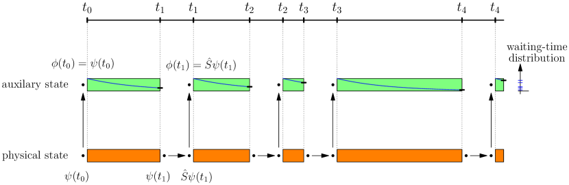
Figure 1: The figure illustrates the time-evolution as generated by the quantum jump algorithm. The lower track represents the piecewise deterministic propagation of the physical state which is intercepted at instances in time where the bath operator $\hat{S}$ acts on the state. The points in time where this takes place are determined by sampling a waiting-time distribution. The sampling is performed by propagating an auxiliary state (represented in the upper track) with a non-Hermitian Hamiltonian. Uniformly distributed random numbers are drawn and once the norm of the auxiliary state drops below the current random number the propagation of the physical and the auxiliary state is suspended. At this point in time the action of the bath operator on the physical state results in a new state which is then also used to initialize the auxiliary state for the evolution. The simulation of both states is then resumed again.

3.2 Quantum Jump Algorithm

We are now left with the actual solution of the stochastic Schrödinger equation (24). In past work, this has been done by directly integrating this equation with standard approaches - e.g., with appropriately modified Runge-Kutta methods (see e.g. [10, 35] and references therein). These approaches are reasonable when we deal with a small number of accessible states or short propagation times. However, they become increasingly unstable with an increasing number of states or for very long timescales, which is the case for realistic systems, like molecular structures, surfaces or solids. As an alternative, we have thus adopted the quantum jump algorithm pioneered in the work of Diósi [36], Dalibard [37], Zoller and Gardiner and collaborators [38, 39, 40] as well as Carmichael [41]. At the price of introducing the propagation of auxiliary states, the quantum jump algorithm provides improved stability for systems with a large number of states/particles and, due to the piecewise deterministic evolution, also a stable propagation scheme for long timescales.

This algorithm works as follows. Consider the deterministic time-evolution given by the follwing norm-preserving non-linear Schrödinger equation

$$\frac{d}{dt}\psi_{j}(t)=-i\left(\hat{\cal H}_{S}+\frac{i}{2}||\hat{S}\psi||^{2}\right)\psi_{j}(t),$$ (54)

where the non-Hermitian Hamiltonian ${\cal H}_{S}$ is given by

$$\hat{\cal H}_{S}=\hat{H}_{S}-\frac{i}{2}S^{\dagger}S.$$ (55)

As before, the operators $\hat{H}_{S}$ and $\hat{S}$ denote the Hermitian system Hamiltonian and the bath operator of Eq. (24) . The main objective of the quantum jump algorithm is to sample the stochastic process given by Eq. (24) in terms of a piecewise deterministic evolution, i.e. a set of deterministic time intervals generated by the evolution of Eq. (54) and action of the bath operator $\hat{S}$ between two consecutive time intervals. A central ingredient of the algorithm is a waiting-time distribution which determines when the jumps (i.e., actions of the bath operator) appear throughout the simulation.

In order to sample the unknown waiting-time distribution, an auxiliary set of wavefunctions $\phi_{j}^{\rm aux}$ is introduced. The wavefunctions $\phi_{j}^{\rm aux}$ are propagated with the non-Hermitian Hamiltonian $\hat{\cal H}_{S}$ alongside the actual states $\psi_{j}$. Since the auxiliary system evolves with a non-Hermitian Hamiltonian, the norm of the states $\phi_{j}^{\rm aux}$ is not preserved. It can be shown [16] that the decay of the norm of the auxilary wavefunctions is related to the waiting-time distribution. The algorithm makes use of this fact and directly samples the waiting-time distribution on the fly from the norm decay.

In terms of the Kohn-Sham system, the steps of the algorithm can then be summarized as follows

• Draw a uniform random number $\eta_{k}\in[0,1]$ for the Kohn-Sham Slater determinant

• Propagate $N$ auxiliary orbitals $\phi_{j}^{\rm aux}$ under the non-Hermitian dynamics

  $$i\partial_{t}\phi_{j}^{\rm aux}=\left[{\hat{H}}_{\rm KS}-\frac{i}{2}{\hat{S}}^{\dagger}{\hat{S}}\right]\phi_{j}^{\rm aux},\qquad j=1\ldots N$$

• Propagate the orbitals $\psi_{j}^{\rm KS}$, $j=1\ldots N$ of the Kohn-Sham system with a norm-conserving dynamics according to

  $$i\partial_{t}\psi_{j}^{\rm KS}=\left[{\hat{H}}_{\rm KS}-\frac{i}{2}{\hat{S}}^{\dagger}{\hat{S}}+i||\hat{S}\psi_{j}^{\rm KS}||^{2}\right]\psi_{j}^{\rm KS}$$

• If the norm of the Kohn-Sham Slater determinant drops below the drawn random number $\eta_{j}$, act with the bath operator(s) on the Kohn-Sham orbitals and update the auxiliary orbitals

  $$||\mbox{Det}\{\phi_{j}^{\rm aux}(t_{k})\}||\leq\eta_{k}\rightarrow\,\, \begin{cases}\psi_{j}^{\rm KS}(t_{k})={\hat{S}}\psi_{j}^{\rm KS}(t_{k})&\\ \phi_{j}^{\rm aux}(t_{k})=\psi_{j}^{\rm KS}(t_{k})&\end{cases}$$

• Go to step 1)

The piecewise deterministic evolution that is generated by the steps of this algorithm is illustrated schematically in Fig. 1.

Averaging at any given time over an ensemble of stochastic realizations allows then to obtain mean values of any physical observable. It is also important to realize that we have a full statistical ensemble at hand. This allows to compute distributions of observables, higher order moments, cumulants, etc. In this sense the ensemble of stochastic realizations generated by the stochastic Schrödinger equation carries more information than the statistical operator, since the latter is merely a first order moment and higher order moments and cumulants cannot be computed easily from the first order moment (if at all).

We also emphasize here, that the interpretation of a single stochastic trajectory is not meaningful: the stochastic realizations have to be considered always as an ensemble. When averages over the stochastic ensemble are performed, the “convergence” of all observables of interest has to be checked carefully by increasing the number of realizations of the stochastic process.

Note that without further constraints the action of the bath operator in step 4) of the algorithm can in principle lead to a loss of orthogonality. For example, all orbitals of the Slater determinant could relax to the same orbital shape. The system could loose in this way its fermionic character. In order to maintain the fermionic nature of the Kohn-Sham state vector, we have to ensure that the orbitals of the Kohn-Sham Slater determinant remain orthogonal. To achieve this, we perform an orthogonalization of the orbitals after each action of the bath operators. This orthogonalization can be thought of as being part of the definition of the action of the operator $\hat{S}$.

From our numerical experience so far, the waiting-time distribution seems to follow mainly a single exponential distribution. It would therefore appear appealing to parametrize this distribution and to draw the waiting times from the analytical expression of the parametrization. In this way the propagation of the auxiliary states could be avoided and a speedup of the propagation by a factor of two could be gained. However, it is not clear if the waiting times of the Kohn-Sham system follow always an exponential distribution. In particular, the shape of the distribution is unknown, when, e.g., ionic motion is involved, or when the system is subject to strong external electric or magnetic fields. Therefore, to be on the safe side, in the present work we always sample the waiting-time distribution by propagating the auxiliary system.

It is also worth noting that the average over stochastic realizations of the ensemble generally converges faster when the system-bath interaction increases. In the opposite limit the convergence is slow. When the system-bath interaction is very weak, only a small damping will be exerted by the ${\hat{S}}^{\dagger}{\hat{S}}$ term in Eq. (2)), and hence it takes longer for the norm of the auxiliary wave functions to drop below their waiting times. This in turn implies that fewer jumps occur and hence more stochastic realizations are required to converge to a smooth observable distribution.

4 Applications

4.1 Finite Systems

In the last section we have introduced technical details for the quantum jump algorithm that we use to simulate the stochastic process associated with the stochastic Kohn-Sham equation, Eq. (47). In this section we apply the algorithm to molecular systems with and without clamped ions. As first example we consider a situation of clamped ionic coordinates. As testcase we investigate a (1,4)-phenylene-linked zincbacteriochlorin-bacteriochlorin complex. Due to an extra Mg atom in the left porphyrin ring of the complex the molecule is not fully symmetric. As a result, the highest-occupied molecular orbital (HOMO) of this molecule is located on the left porphyrin ring, whereas the lowest-unoccupied molecular orbital (LUMO) is located on the right porphyrin ring, cf. Fig. 2.

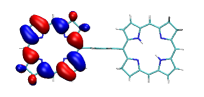
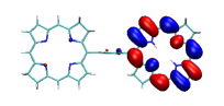
Figure 2: Real part of the HOMO (left panel) and LUMO (right panel) orbitals of (1,4)-phenylene-linked zincbacteriochlorin-bacteriochlorin.

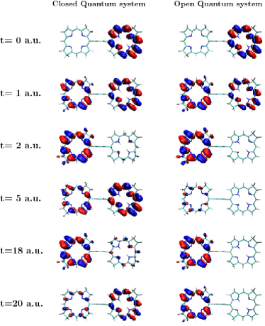
Figure 3: Snapshots of the time evolution of the HOMO orbital of zincbacteriochlorin-bacteriochlorin with clamped ions. The plots display the real part of the orbital. In the left column the closed quantum system evolution is shown at different points in time and the right column displays the evolution of the system with a coupling to a thermal bath. A rather fast relaxation rate of $\tau=1$ a.u. has been used for the bath operator in the open quantum system case.

This system has been used as a model to study charge-transfer excitations in linear response TDDFT [42]. Here instead we consider open and closed system real-time propagation. We prepare the zincbacteriochlorin-bacteriochlorin complex in an entangled initial-state, where the orbital of the HOMO is replaced by

$$\psi_{{}^{\rm HOMO}}^{{}^{\rm TDKS}}(t=0)=\frac{1}{\sqrt{2}}\left[\psi_{{}^{\rm HOMO}}^{{}^{\rm GS}}+e^{-i\frac{\pi}{2}}\psi_{{}^{\rm LUMO}}^{{}^{\rm GS}}\right],$$ (56)

where $\psi_{{}^{\rm HOMO}}^{{}^{\rm GS}}$ and $\psi_{{}^{\rm LUMO}}^{{}^{\rm GS}}$ denote the ground-state HOMO and LUMO, respectively. For all other orbitals the ground-state configuration is used at the initial time. Starting from this excited initial Slater determinant the system is then evolved freely in time without any external fields. For the bath operators we employ the model of Eq. (2.5) introduced in section 2.5 at zero temperature. The dynamics of the system is illustrated in Fig. 3 where we plot the real part of the HOMO orbital for different snapshots in time. The left panel summarizes the closed system evolution and the right panel an ensemble average over 100 stochastic realizations in the open system case. Let us first focus on the closed quantum system case. Due to the entangled initial state in Eq. (56), the time-dependence of the orbital $\psi_{{}^{\rm HOMO}}^{{}^{\rm TDKS}}(t)$ has mainly oscillatory phase contributions $\exp(-i\epsilon_{\rm HOMO}t)$ and $\exp(-i\epsilon_{\rm LUMO}t)$ from the ground-state HOMO and LUMO, respectively. Only small nonlinearities arise due to the dependence of the Kohn-Sham Hamiltonian on the time-dependent density. Since the system is propagated as closed quantum system, the phase oscillations would continue indefinitely.

On the other hand, the open quantum system evolution in the right panel of Fig. 3 shows for $\psi_{{}^{\rm HOMO}}^{{}^{\rm TDKS}}(t)$ a fast relaxation from the entangled initial state back to the HOMO which is localized on the left porphyrin ring. If we now imagine computing Ehrenfest forces from these orbital contributions, it is clear that the forces will differ qualitatively in the closed and open quantum system cases. While in the closed quantum system case the forces will be oscillatory, they will show relaxation behavior similar to the orbitals in the open quantum case. This example emphasizes that the coupling of electronic degrees of freedom to a thermal bath yields qualitatively different forces compared to standard QMD approaches.

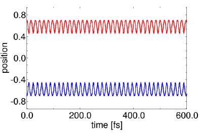
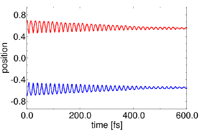
Figure 4: Left panel: Here we show the ionic positions of a Neon dimer as function of time for a closed quantum system. As initial condition we have selected a stretched configuration of the dimer which results in an indefinite coherent oscillation of the two nuclei. Right panel: Using the same initial state we have evolved with SQMD a stochastic ensemble of trajectories. Shown is the average of the nuclear positions for an ensemble with 100 stochastic realizations. As relaxation time for the simulation we have employed $\tau=300$ fs. The ionic velocities follow a Maxwell-Boltzmann distribution with a temperature of 290K.

This observation motivates our second example, where we consider a stochastic QMD simulation for a neon dimer. In this case the ions are not clamped at the equilibrium configuration. Instead we use stretched initial positions for the ions of the dimer as initial state for the open and closed system propagation. If we would treat the ions quantum mechanically, then the bath operators would also act on the nuclear wavefunctions. However, since we have restricted ourselves here to the limit of classical ions we replace this action of the bath operators by modifying the velocities of the ions. At every occasion when the bath operators act on the electronic wavefunctions we draw new velocities for the ions from a Maxwell-Boltzmann distribution. This is a simple approach but can be improved with e.g., recently introduced stochastic thermostats for the ions [22].

In the left panel of figure Fig. 4 we show the ionic positions of the dimer as function of time for a standard Ehrenfest TDDFT closed quantum system evolution. In the right panel we display for the same initial conditions the open quantum system evolution within SQMD. For the SQMD simulation we have employed a relaxation time of $\tau=300$ fs and an average over 100 stochastic trajectories has been performed which results in a smooth decay of the nuclear oscillations.

4.2 Extended Systems

So far we have considered only finite molecular systems. However, a large class of applications requires also the treatment of periodic boundary conditions in one, two or three dimensions. This includes for example decoherence and dissipation in nanowires, electronic relaxation on surfaces, or hot electron thermalization in bulk systems. For these cases it is desirable to extend our approach to periodic systems. In this section we briefly discuss the necessary steps in order to apply SQMD to extended systems.

There are some extra details and conditions that have to be satisfied in order to treat periodic systems with SQMD. As a first step we expand the stochastic Kohn-Sham orbitals of the periodic system of interest in the complete set of the corresponding ground-state Bloch-orbitals $\varphi_{k}(\underline{\bf r})$

$$\psi_{k}(\underline{\bf r},t)=\sum_{k^{\prime}}d_{k^{\prime}}(t)\varphi_{k^{\prime}}(\underline{\bf r}).$$ (57)

This gives rise to stochastic expansion coefficients $d_{k}(t)$ which are then propagated in time using, e.g., the quantum jump algorithm that we have presented in section 3.2. Similar to the case of molecules, the fermionic nature of the electronic subsystem needs to be taken into account by orthogonalizing the occupied states after each application of the bath operator (cf. step (4) of the quantum jump algorithm).

In addition, care has to be taken for the choice of gauge for the vector and scalar potentials in the Hamiltonian of the extended system. Here, the same restrictions apply as in standard closed-system TDDFT simulations. In practice, we consider only purely time-dependent vector potentials which retain the periodicity of the considered system at all times. In the present context we have to assume in addition that the bath operators retain the periodicity of the extended system as well. This restricts the choice of baths represented by local operators that satisfy the condition

$$\hat{S}(\underline{\bf r})=\hat{S}(\underline{\bf r}+{\bf R})$$ (58)

where ${\bf R}$ denotes the usual displacement vector of the unit cell. This may exclude certain relaxation mechanisms. However, the importance of these relaxation and dephasing channels can always be checked by increasing the size of the supercell that is used in the simulation.

While we do not have fully implemented this scheme yet, we want to argue about important physical processes that can be studied with this approach. For instance, one could study adsorption of molecules on surfaces whose opposite side is set on a thermal stage that keeps the electron and/or ion temperatures fixed. Again, this could be accomplished in a supercell geometry by coupling some “bulk” layers away from the surface with a local operator that maintains energy equilibrium in that region (an example of such operator is given in Ref. [43]). The rest of the system is let to follow its own dynamics. If we excite the molecules and/or surface - e.g., by application of a short electromagnetic field - electrons and ions can then distribute energy and momentum first in the layers adjacent to the surface and then relax energy into the bath, where they would thermalize to the appropriate canonical distributions. Analogously, we could monitor energy relaxation of electrons and ions in a bulk exited either thermally or electrically and kept at a given temperature by a thermal stage. Important phenomena that are then accessible would be, e.g., phase transitions driven by dissipative effects.

5 Conclusions

In summary, we have presented a detailed account of stochastic quantum molecular dynamics. The approach is based on a stochastic Schrödinger equation, which may or may not describe Markovian dynamics - although we have focused the discussion to the Markovian case. Our approach allows us to describe the dynamics of electrons and ions coupled to one or many external environments. For simplicity we have restricted our examples to the situation of classical ions, but the approach is, in principle, valid also for quantum ions. Although we have not reported any actual implementation of SQMD for periodic systems, we have outlined the theory behind its extension to this important case. Work along these lines is in progress and will be reported elsewhere [14].

This approach is thus amenable to studying many interesting phenomena related to energy relaxation and dephasing of the electronic subsystem in the presence of ionic dynamics, such as local ionic and electronic heating in laser fields, relaxation processes in photochemistry, etc., a feature that is lacking in any “standard” molecular dynamics approach.

We acknowledge support from DOE under grant DE-FG02-05ER46204 and Lockheed Martin.

References

- [1] M. A. L. Marques, C. A. Ullrich, F. Nogueira, A. Rubio, K. Burke, E. K. U. Gross, Time-Dependent Density Functional Theory (Lecture Notes in Physics), Springer-Verlag, Berlin, 2006.
- [2] M. Di Ventra, T. N. Todorov, Transport in nanoscale systems: the microcanonical versus grand-canonical picture, J. Phys. Cond. Mat. 16 (2004) 8025.
- [3] N. Bushong, N. Sai, M. Di Ventra, Approach to steady-state transport in nanoscale conductors, Nano Letters 5 (2005) 2569.
- [4] K. Burke, R. Car, R. Gebauer, Density Functional Theory of the Electrical Conductivity of Molecular Devices, Phys. Rev. Lett. 94 (2005) 146803.
- [5] S. Kurth, G. Stefanucci, E. Khosravi, C. Verdozzi, E. K. U. Gross, Dynamical coulomb blockade and the derivative discontinuity of time-dependent density functional theory, Phys. Rev. Lett. 104 (2010) 236801.
- [6] F. D. Vila, D. A. Strubbe, Y. Takimoto, X. Andrade, A. Rubio, S. G. Louie, J. J. Rehr, Basis set effects on the hyperpolarizability of chcl[sub 3]: Gaussian-type orbitals, numerical basis sets and real-space grids, J. Chem. Phys. 133 (2010) 034111.
- [7] M. Petersilka, E. K. U. Gross, Strong-field double ionization of helium: A density-functional perspective, Laser Phys. 9 (1999) 105.
- [8] T. Kreibich, N. Gidopoulos, R. van Leeuwen, E. Gross, Towards time-dependent density-functional theory for molecules in strong laser pulses, Prog. Theor. Chem. and Phys. 14 (2003) 69.
- [9] M. Di Ventra, R. D’Agosta, Stochastic time-dependent current-density-functional theory, Phys. Rev. Lett. 98 (2007) 226403.
- [10] R. D’Agosta, M. Di Ventra, Stochastic time-dependent current-density-functional theory: A functional theory of open quantum systems, Phys. Rev. B 78 (2008) 165105.
- [11] X. Zheng, G. Chen, Y. Mo, S. Koo, H. Tian, C. Yam, Y. Yan, Time-dependent density functional theory for quantum transport, J Chem. Phys. 133 (2010) 114101.
- [12] J. Yuen-Zhou, C. Rodríguez-Rosario, A. Aspuru-Guzik, Time-dependent current-density functional theory for generalized open quantum systems, Phys. Chem. Chem. Phys. 11 (2009) 4509.
- [13] H. Appel, M. Di Ventra, Stochastic quantum molecular dynamics, Phys. Rev. B 80 (2009) 212303.
- [14] H. Appel, M. Di Ventra, Stochastic relaxation in periodic systems, In preparation.
- [15] N. G. V. Kampen, Stochastic Processes in Physics and Chemistry, Elsevier Science and Technology, 3rd Ed., 2007.
- [16] H. P. Breuer, F. Petruccione, The Theory of Open Quantum Systems, Oxford University Press, Oxford, 2002.
- [17] U. Weiss, Quantum Dissipative Systems (Series in Modern Condensed Matter Physics), World Scientific Publishing Company; 3 edition, 2008.
- [18] P. Gaspard, M. Nagaoka, Non-markovian stochastic Schrödinger equation, J. Chem. Phys. 111 (1999) 5676.
- [19] H. Feshbach, Unified theory of nuclear reactions, Annals of Physics 5 (1958) 357.
- [20] S. Nordholm, S. A. Rice, A quantum ergodic theory approach to unimolecular fragmentation, J. Chem. Phys. 62 (1975) 157.
- [21] S. Kurth, G. Stefanucci, C.-O. Almbladh, A. Rubio, E. K. U. Gross, Time-dependent quantum transport: A practical scheme using density functional theory, Phys. Rev. B 72 (2005) 035308.
- [22] G. Bussi, D. Donadio, M. Parrinello, Canonical sampling through velocity rescaling, J. Chem. Phys. 126 (2007) 014101.
- [23] G. Lindblad, On the generators of quantum dynamical semigroups, Commun. Math. Phys. 48 (1976) 119.
- [24] C. Gardiner, Stochastic Methods: A Handbook for the Natural and Social Sciences, Springer Series in Synergetics, Vol. 13, 2nd ed., 1985.
- [25] R. Balian, From microphysics to macrophysics, Springer, Berlin, 1991.
- [26] M. Di Ventra, Electrical transport in nanoscale systems, Cambridge University Press, Cambridge, 2008.
- [27] M. Di Ventra, R. D’Agosta, Comment on ”time-dependent current-density functional theory for generalized open quantum systems” by J. Yuen-Zhou, C. Rodriiguez-Rosario and A. Aspuru-Guzik, arXiv http://arxiv.org/abs/0911.3932 (2009) 3.
- [28] S. Maniscalco, F. Intravaia, J. Piilo, A. Messina, Misbeliefs and misunderstandings about the non-markovian dynamics of a damped harmonic oscillator, Journal of Optics B: Quantum and Semiclassical Optics 6 (2004) S98.
- [29] T. Kreibich, E. K. U. Gross, Multicomponent density-functional theory for electrons and nuclei, Phys. Rev. Lett. 86 (2001) 2984.
- [30] Y. V. Pershin, Y. Dubi, M. Di Ventra, Effective single-particle order- scheme for the dynamics of open noninteracting many-body systems, Phys. Rev. B 78 (2008) 054302.
- [31] N. Bushong, M. Di Ventra, The decay of excited He from stochastic density-functional theory: a quantum measurement theory interpretation, J. Phys. Cond. Mat. 20 (2008) 395214.
- [32] M. Di Ventra, S. T. Pantelides, Hellmann-feynman theorem and the definition of forces in quantum time-dependent and transport problems, Phys. Rev. B 61 (2000) 16207.
- [33] A. Castro, et al., octopus: a tool for the application of time-dependent density functional theory, phys. stat. sol. B 243 (2006) 2465.
- [34] W. Magnus, On the exponential solution of differential equations for a linear operator, Comm. Pure Appl. Math. 7 (1954) 649.
- [35] P. E. Kloeden, E. Platen, Numerical Solution of Stochastic Differential Equations (Stochastic Modelling and Applied Probability), Springer, Berlin, 1992.
- [36] L. Diosi, Quantum stochastic processes as models for state vector reduction, Journal of Physics A: Mathematical and General 21 (1988) 2885.
- [37] J. Dalibard, Y. Castin, K. Mølmer, Wave-function approach to dissipative processes in quantum optics, Phys. Rev. Lett. 68 (1992) 580.
- [38] R. Dum, A. S. Parkins, P. Zoller, C. W. Gardiner, Monte carlo simulation of master equations in quantum optics for vacuum, thermal, and squeezed reservoirs, Phys. Rev. A 46 (1992) 4382.
- [39] C. W. Gardiner, A. S. Parkins, P. Zoller, Wave-function quantum stochastic differential equations and quantum-jump simulation methods, Phys. Rev. A 46 (1992) 4363.
- [40] R. Dum, P. Zoller, H. Ritsch, Monte carlo simulation of the atomic master equation for spontaneous emission, Phys. Rev. A 45 (1992) 4879.
- [41] H. J. Carmichael, S. Singh, R. Vyas, P. R. Rice, Photoelectron waiting times and atomic state reduction in resonance fluorescence, Phys. Rev. A 39 (1989) 1200.
- [42] A. Dreuw, M. Head-Gordon, Failure of time-dependent density functional theory for long-range charge-transfer excited states: The zincbacteriochlorin-bacteriochlorin and bacteriochlorophyll-spheroidene complexes, J. Am. Chem. Soc. 126 (2004) 4007.
- [43] Y. Dubi, M. Di Ventra, Thermoelectric effects in nanoscale junctions, Nano Letters 9 (2009) 97.