Subtlety of Studying the Critical Theory of a Second Order Phase Transition

Abstract

We study the quantum phase transition from a super solid phase to a solid phase of $\rho=1/2$ for the extended Bose-Hubbard model on the honeycomb lattice using first principles Monte Carlo calculations. The motivation of our study is to quantitatively understand the impact of theoretical input, in particular the dynamical critical exponent $z$, in calculating the critical exponent $\nu$. Hence we have carried out four sets of simulations with $\beta=2N^{1/2}$, $\beta=8N^{1/2}$, $\beta=N/2$, and $\beta=N/4$, respectively. Here $\beta$ is the inverse temperature and $N$ is the numbers of lattice sites used in the simulations. By applying data collapse to the observable superfluid density $\rho_{s2}$ in the second spatial direction, we confirm that the transition is indeed governed by the superfluid-insulator universality class. However we find it is subtle to determine the precise location of the critical point. For example, while the critical chemical potential $(\mu/V)_{c}$ occurs at $(\mu/V)_{c}=2.3239(3)$ for the data obtained using $\beta=2N^{1/2}$, the $(\mu/V)_{c}$ determined from the data simulated with $\beta=N/2$ is found to be $(\mu/V)_{c}=2.3186(2)$. Further, while a good data collapse for $\rho_{s2}N$ can be obtained with the data determined using $\beta=N/4$ in the simulations, a reasonable quality of data collapse for the same observable calculated from another set of simulations with $\beta=8N^{1/2}$ can hardly be reached. Surprisingly, assuming $z$ for this phase transition is determined to be 2 first in a Monte Carlo calculation, then a high quality data collapse for $\rho_{s2}N$ can be achieved for $(\mu/V)_{c}\sim 2.3184$ and $\nu\sim 0.7$ using the data obtained with $\beta=8N^{1/2}$. Our results imply that one might need to reconsider the established phase diagrams of some models if the accurate location of the critical point is crucial in obtaining a conclusion.

I Introduction

Searching and investigating models in which one might observe a supersolid phase (SS) has been one of the central research interests in condensed matter physics recently. Indeed, it is reported numerically that several spin models and extended Bose-Hubbard models provide convincing evidence for the existence of a supersolid state, where the long range superfluid order and solid order coexist Sen05 ; Wes05 ; Mel05 ; Bon05 ; Mel06 ; Ng06 ; Sen07 ; Gan07_1 ; Wes07 ; Gan07_2 ; Laf07 ; Che08 . For example, a Monte Carlo investigation of bilayer spin-1/2 Heisenberg model with an external uniform magnetic field on the square lattice demonstrates that a field-induced supersolid phase can be stabilized when the magnitude of the external magnetic field takes certain values Ng06 ; Laf07 . A supersolid phase is observed numerically by considering interacting bosons as well Sen05 ; Wes05 ; Mel05 ; Bon05 ; Mel06 ; Gan07_1 ; Wes07 ; Gan07_2 ; Che08 . Further, it is expected that SS and the quantum phase transitions out of SS might be realized experimentally using ultracold atoms on optical lattices Gre02 ; Sto04 ; Blo06 . Although rich phase diagrams have been obtained for both spin models and extended Bose-Hubbard models, a detailed investigation of the nature of the phase transitions out of SS is available only for bilayer spin-1/2 Heisenberg model on the square lattice. Further, despite the fact that the bilayer spin-1/2 Heisenberg model can be mapped into the hard-core Bose-Hubbard model, it is known that both the hard-core Bose-Hubbard model on the square and the honeycomb lattices do not exhibit a stable SS phase in the $t/V$-$\mu/V$ phase diagram at a fixed $U/t$ Wes07 ; Bat00 . Here $t$ is the nearest-neighbor hopping parameter, $\mu$ is the chemical potential, $V$ is a nearest-neighbor repulsion, and $U$ stands for an onsite repulsion. As a consequence, it will be interesting to carry out an investigation on the nature of quantum phase transitions out of SS for the extended Bose-Hubbard model. Finally, considering the many noticeable properties of graphene Nov04 ; Nov05 ; Zha05 ; Cas09 , for which the underlying lattice is a honeycomb lattice, as well as the fact that quantum fluctuations are expected to be more relevant on the honeycomb lattice due to its coordination number, in this paper we study the phase transition from a SS phase to a solid state of $\rho=1/2$ for the extended Bose-Hubbard model on the honeycomb lattice using first principles Monte Carlo simulations. Here $\rho$ refers to the average number of bosons per lattice site.

The nature of quantum phase transitions out of a SS to a superfluid and a solid phases have been studied quantitatively using first principles unbiased quantum Monte Carlo method for the bilayer spin-1/2 Heisenberg model Laf07 . Indeed it is demonstrated convincingly that the critical theories determined from the Monte Carlo data are consistent with the theoretical prediction Laf07 . For example, by applying the technique of data collapse to the observable superfluid density $\rho_{s}$, one reaches a perfect agreement between the numerical data and the theoretical prediction of superfluid-insulator universality class for the phase transition from a SS to a solid state Fis89 ; Ale04 . To obtain the ground-state phase diagrams of the desired models using finite temperature Monte Carlo algorithms, in particular to quantitatively study the nature of the phase transitions in the phase diagrams, one useful strategy is to scale the inverse temperature $\beta$ by the relation $\beta=cL^{z}$ in the simulations. Here in addition to the dynamical critical exponent $z$ which is already introduced earlier, $L$ and $c$ appearing in $\beta=cL^{z}$ are the box sizes used in the simulations and a constant, respectively. Surprisingly, despite the fact that the correct way to determine the critical theory for a second order phase transition is to employ the relation $\beta=cL^{z}$ in the simulations, several studies seem to simply use $\beta=cL$ and ignore the impact of the dynamical critical exponent $z$ when obtaining the ground-state phase diagrams. Whether the strategy of using $\beta=cL$ instead of $\beta=cL^{z}$ in the Monte Carlo calculations has noticeable influence on determining the critical theory for a second order phase transition remains to explore.

The motivation of our investigation on the quantum phase transition from a supersolid state to a solid state of $\rho=1/2$ by varying $\mu/V$ at fixed $U/t=20$ and $t/V=0.16$ in the parameter space for the extended Bose-Hubbard model is twofold. First of all, we would like to determine the critical chemical potential $(\mu/V)_{c}$ as precise as possible since such a study is useful in calculating critical exponents such as $\beta$ ($\beta/\nu$) and $\eta$. Secondly, since one should scale the inverse temperature $\beta$ with the system size for the phase transition considered here due to the theoretical prediction $z=2$, we would like to understand the impact of scaling $\beta$ linearly with the linear length of the system on studying the corresponding critical theory of this transition. Indeed as we will demonstrate later, scaling $\beta$ linearly with the system linear length either leads to poor data collapse for the observables measured in this study, or one would arrive at a different critical theory than the expected one.

This paper is organized as follows. After a brief description of the motivation behind this study, the extended Bose-Hubbard model considered here as well as the observables measured in our Monte Carlo simulations are introduced. Follows that we present our numerical results. In particular, the corresponding critical point is determined with high precision by the method of data collapse. The subtlety of determining the critical theory for the transition from a SS phase to a solid state of $\rho=1/2$ is demonstrated as well. Finally, a section is devoted to conclude our investigation.

II The Model and Observables

The extended Bose-Hubbard model considered in this study is given by

$$H = -t\sum_{\langle i,j\rangle}\left(b^{\dagger}_{i}b_{j}+b^{\dagger}_{j}b_{i}\right)+\frac{U}{2}\sum_{i}n_{i}(n_{i}-1)$$ (1)

$$+V\sum_{\langle i,j\rangle}n_{i}n_{j}-\mu\sum_{i}n_{i},$$

where $b^{\dagger}_{i}$ ($b_{i}$) are the bosonic creation (annihilation) operators at site $i$ and $n_{i}$ is the occupation number at lattice site $i$. Further, $U$, $V$, $t$, and $\mu$ appearing in Eq. (1) are defined as before.

The honeycomb lattice with periodic spatial boundary conditions implemented in our simulations is depicted in figure 1. The dashed rectangle in figure 1, which contains $4$ spins, is the elementary cell for building a periodic honeycomb lattice covering a rectangular area. For instance, the honeycomb lattice shown in figure 1 contains 3 $\times$ 3 elementary cells. The lattice spacing $a$ is the distance between two neighboring sites. The honeycomb lattice is not a Bravais lattice. Instead it consists of two triangular Bravais sub-lattices $A$ and $B$ (depicted by solid and open circles in figure 1). As a consequence, the momentum space of the honeycomb lattice is a doubly-covered Brillouin zone of the two triangular sub-lattices.

Following earlier works in Wes07 ; Gan07_2 , our primary interest for the model described by Eq. (1) is to study the phase transitions from a supersolid phase to a solid phase of $\rho=1/2$ and from a superfluid phase to a Mott insulator phase of $\rho=1$ by varying the chemical potential $\mu/V$ at fixed $U/t=20$ and $t/V=0.16$ in the parameter space. In particular we would like to determine the critical chemical potentials $(\mu/V)_{c}$ as well as the correlation length critical exponents $\nu$ and dynamical critical exponents $z$ for these two phase transitions accurately. To fulfill these tasks, we have measured the superfluid density $\rho_{si}=\langle W_{i}^{2}\rangle/\beta$ with $i\in\{1,2\}$ in our simulations and have focused on the finite-size scaling of $\rho_{s2}N^{z/2}$. Here $\langle W_{i}^{2}\rangle$ is the winding number fluctuation in $i$-direction.

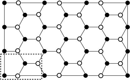
Figure 1: The periodic honeycomb lattice consisting of two triangular sub-lattices A and B, which are depicted by solid and open circles, respectively. The dashed rectangle is an elementary cell for building a periodic honeycomb lattice covering a rectangular area.

III Determination of the critical point

To determine the location of the critical point in the parameter space $\mu/V$, one useful technique is to study the finite-size scaling of certain observables. For example, if the transition is second order, then near the transition, the observable $\rho_{si}N^{z/2}$ for $i\in\{1,2\}$ should be described well by the following finite-size scaling ansatz

$${\cal O}_{N}(j)=g_{{\cal O}}(jN^{1/2\nu},N^{z/2}/\beta),$$ (2)

where ${\cal O}_{N}$ stands for $\rho_{si}N^{z/2}$, $j=(\mu_{c}-\mu)/\mu_{c}$, and $\nu$ is the critical exponent corresponding to the correlation length $\xi$. Finally $g_{{\cal O}}$ appearing above is a smooth function of the variables $jN^{1/2\nu}$ and $N^{z/2}/\beta$. In writing Eq. (2), we have ignored explicitly the confluent correction to the scaling. Taking this correction into account, one concludes that for large enough $\beta$ when the finite-temperature effects can be ignored, the curves of different $N^{1/2}$ for ${\cal O}_{N}$, as functions of $\mu/V$, should have the tendency to intersect at critical point $(\mu/V)_{c}$ for large $N^{1/2}$. Theoretically, it is predicted that the transition from a supersolid phase to a solid phase of $\rho=1/2$ for this model is governed by the superfluid-insulator universality class, namely one has $\nu=0.5$, $\beta=0.5$ and $z=2$ Fis89 ; Ale04 . In the following we will apply the finite-size scaling formula, Eq. (2), to the observable $\rho_{s2}L$ to determine $(\mu/V)_{c}$. In particular, we would like to examine whether the theoretical prediction is consistent with our Monte Carlo data.

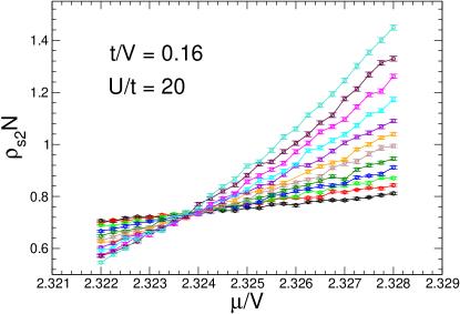
Figure 2: Monte Carlo data of $\rho_{s2}N$ as functions of $\mu/V$ for the quantum phase transition from a supersolid state to a solid state of $\rho=1/2$. For a given fixed $N$, the inverse temperature $\beta$ used for this set of simulations is given by $\beta=2N^{1/2}$.

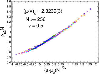
Figure 3: Data collapse for the observable $\rho_{s2}N$ with $16^{2}\leq N\leq 32^{2}$ for the quantum phase transition from a supersolid state to a solid state of $\rho=1/2$. The data is calculated using $\beta=2N^{1/2}$. In obtaining the figure, the critical exponent $\nu$ is fixed to be the expected theoretical value $\nu=0.5$.

To study the critical theory for the phase transition of our central interest, we have performed large scale Monte Carlo simulations using the directed loop algorithms available in the ALPS library ALP07 . Without losing the generality, in our simulations we have fixed $V$ to be $1.0$ and have varied $\mu$. To determine $(\mu/V)_{c}$ using the finite-size scaling ansatz Eq. (2), one needs to use large enough $\beta$ so that the finite-temperature effects are negligible. For this purpose, we have carried out a trial simulation at $\mu/V=2.53$ with $N=14^{2}$ and we have found that one already obtains the zero-temperature result for $\rho_{s2}$ using $\beta=2\times 14^{1/2}$. Hence we use $\beta=2N^{1/2}$ in other simulations as well. Notice the strategy of applying $\beta=2N^{1/2}$ or similar ones for a fixed $N^{1/2}$ in the simulations was used in many studies exploring the phase diagrams of certain models in the literature. After determining the relation $\beta=2N^{1/2}$ which allows one to access zero-temperature values for the observable $\rho_{s2}$, we have further carried out large scale simulations with $N$ ranging from $N=10^{2}$ to $N=32^{2}$. Figure 2 demonstrates the results of $\rho_{s2}N$ as functions of $\mu/V$ for this set of simulations. The figure indicates that the phase transition is likely a second order transition because the curves of different $N^{1/2}$ have the tendency to intersect at a particular $\mu/V$ is the parameter space. Using fixed $z=2$ and $\nu=0.5$, the best result of data collapse for $\rho_{s2}N$ is reached with $(\mu/V)_{c}=2.3239(3)$ for the data of lattice sizes $16^{2}\leq N\leq 32^{2}$ (figure 3). The quality of data collapse shown in figure 3 is not good, but acceptable. One might attribute the poor quality shown in figure 3 to a correction in Eq. (2) that is not taken into account in our analysis. At this stage, one would naturally conclude that our Monte Carlo data is consistent with the theoretical prediction, namely the critical exponent $\nu$ and dynamical critical exponent $z$ of the phase transition considered above is governed by $\nu=0.5$ and $z=2$.

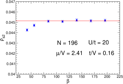
Figure 4: $\rho_{s2}$ as a function of $\beta$ at $\mu/V=2.41$ and $N=196$.

To make sure that we indeed obtain the ground-state properties of the model, we repeat above analysis by firstly determining the required $\beta$ for reaching the ground-state value of $\rho_{s2}$ at $\mu/V=2.41$ and $N=14^{2}$. Surprisingly, we find that one has to use $\beta\sim 6N^{1/2}$ in order to reach the zero-temperature value of $\rho_{s2}$ (figure 4). Because of this observation, we have performed another set of simulations using $\beta=8N^{1/2}$. The results of $\rho_{s2}N$ as functions of $\mu/V$ for this new set of runs is shown in figure 5. By comparing figures 2 and 5, one clearly observes a statistically difference between the critical chemical potentials calculated from these two set of data. To make the discrepancy between these two critical chemical potentials more transparent, we additionally simulating the model using $\beta=2N^{1/2}$ in the range $2.316\leq\mu/V\leq 2.32075$ where $(\mu/V)_{c}$ for the second set of data (which are determined with $\beta=8N^{1/2}$) is located. Figure 6 shows the results of $\rho_{s2}N$ as functions of $\mu/V$ for these new runs. No intersection between the curves of different $N^{1/2}$ shown in figure 6 confirms our observation that the $(\mu/V)_{c}$ for these two set of data are statistically different.

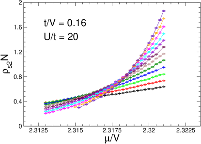
Figure 5: Monte Carlo data of $\rho_{s2}N$ as functions of $\mu/V$ for the quantum phase transition from a supersolid state to a solid state of $\rho=1/2$. For a given fixed $N$, the inverse temperature $\beta$ used for this set of simulations is given by $\beta=8N^{1/2}$.

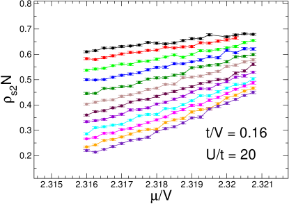
Figure 6: Monte Carlo data of $\rho_{s2}N$ as functions of $\mu/V$ in the range $2.316\leq\mu\leq 2.32075$ with $10^{2}\leq N\leq 32^{2}$. For a given fixed $N$, the inverse temperature $\beta$ used for this set of simulations is given by $\beta=2N^{1/2}$.

After demonstrating that the critical chemical potentials determined from the sets of data obtained using $\beta=2N^{1/2}$ and $\beta=8N^{1/2}$ are statistically different, let us return to the analysis of the second set of $\rho_{s2}$ data. Yet another surprise we find is that a good data collapse for $\rho_{s2}N$ can hardly be achieved if data points of small $N$ are included in the analysis. Only with data of large $N$, namely $N\geq 24^{2}$, a reasonable data collapse for $\rho_{s2}N$ with a fixed $\nu=0.5$ can be obtained given that $(\mu/V)_{c}=2.3185(2)$ (figure 7). The results presented so far in this study raise an interesting question, namely what values of $\beta$ should be used in our simulations in order to obtain the ground-state values for the observable $\rho_{s2}$. In other words, should one perform another set of simulations with even larger values of $\beta$? Actually by examining the relevant finite-size scaling ansatz Eq. (2) carefully, one would realize that the correct strategy is to scale $\beta$ with $N$. Figure 8 shows the results of $\rho_{s2}N$ obtained with $\beta=N/2$ as functions of $\mu/V$. The tendency of crossing between curves of different $N^{1/2}$ shown in figure 8 is much stronger compared to those presented in figures 2 and 5. Finally the quality of data collapse for $\rho_{s2}N$ demonstrated in figure 9 which are obtained from the set of simulations using $\beta=N/2$ is also much better than those found in figures 3 and 7. Notice the $(\mu/V)_{c}$ determined from the data simulated with $\beta=N/2$ is given by $(\mu/V)_{c}=2.3186(2)$ which agrees with $(\mu/V)_{c}=2.3185(2)$, but is statistically different from $(\mu/V)_{c}=2.3239(3)$ obtained earlier from the data determined using $\beta=2N^{1/2}$.

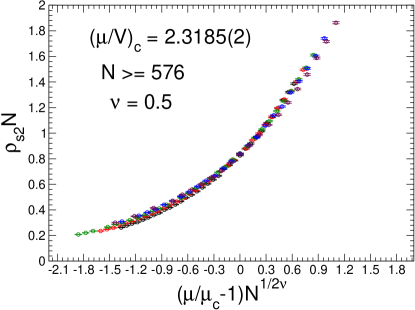
Figure 7: Data collapse of the observable $\rho_{s2}N$ with $24^{2}\leq N\leq 32^{2}$ for the quantum phase transition from a supersolid state to a solid state of $\rho=1/2$. The data is calculated using $\beta=8N^{1/2}$. In obtaining the figure, the critical exponent $\nu$ is fixed to be the expected theoretical value $\nu=0.5$.

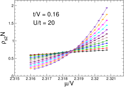
Figure 8: Monte Carlo data of $\rho_{s2}N$ as functions of $\mu/V$ for the quantum phase transition from a supersolid state to a solid state of $\rho=1/2$. For a given fixed $N$, the inverse temperature $\beta$ used for this set of simulations is given by $\beta=N/2$.

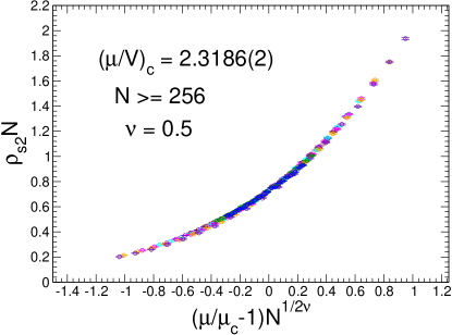
Figure 9: Data collapse of the observable $\rho_{s2}N$ with $16^{2}\leq N\leq 32^{2}$ for the quantum phase transition from a supersolid state to a solid state of $\rho=1/2$. The data is calculated using $\beta=N/2$. In obtaining the figure, the critical exponent $\nu$ is fixed to be the expected theoretical value $\nu=0.5$.

Of course, one might argue that since $N/2>8N^{1/2}$ in the range of $N$ used in the simulations and analysis, the better results shown in figures 8 and 9 than those in figures 2, 3, 5, and 7 is simply because one reaches the ground-state values of $\rho_{s2}$ for the set of data determined using $\beta=N/2$ and the $\rho_{s2}$ data points calculated with $\beta=8N^{1/2}$ still receive finite-temperature effects. To rule out such a possibility, we have performed another set of simulations using $\beta=N/4$ with which the condition $N/4\leq 8N^{1/2}$ is satisfied for $N^{1/2}=18,20,...,32$. Figures 10 and 11 show the results of $\rho_{s2}N$ with $18^{2}\leq N\leq 32^{2}$ for these new simulations using $\beta=N/4$ as functions of $\mu/V$ and the corresponding results of data collapse. In obtaining figure 11, the critical exponent $\nu$ is fixed to $\nu=0.5$ as before. Again the quality of crossing and data collapse seen in figures 10 and 11 are much better than those in figures 5 and 7. To make the comparison on the same footing, figure 12 shows the results of data collapse for $\rho_{s2}N$ determined using $\beta=8N^{1/2}$ with $18^{2}\leq N\leq 32^{2}$. Figures 11 and 12 clearly indicate that the quality of data collapse in figure 11 is much better than that of figure 12. Interestingly, assuming $z=2$ is determined first in a Monte Carlo calculation before one performs the large scale simulations for obtaining $\rho_{s2}$ using $\beta=8N^{1/2}$, then a good data collapse can be reached with $(\mu/V)_{c}=2.3184$ and $\nu=0.7$ using the data of $\rho_{s2}N(N\geq 24^{2})$ calculated with $\beta=8N^{1/2}$ (figure 13). While $(\mu/V)_{c}=2.3184$ is consistent with $(\mu/V)_{c}=2.3185(2)$ and $(\mu/V)_{c}=2.3186(2)$, the $\nu=0.7$ we find is significantly different from the theoretical expectation $\nu=0.5$. Without the theoretical input $\nu=0.5$, one might be misled by figure 13 to conclude an unconventional phase transition is observed for this model. Our results presented in this study clearly imply the importance of using the correct relation for $\beta$ and $N^{1/2}$ in investigating the critical theory of a second order phase transition.

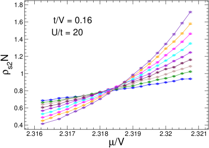
Figure 10: Monte Carlo data of $\rho_{s2}N$ as functions of $\mu/V$ for the quantum phase transition from a supersolid state to a solid state of $\rho=1/2$. For a given fixed $N$, the inverse temperature $\beta$ used for this set of simulations is given by $\beta=N/4$.

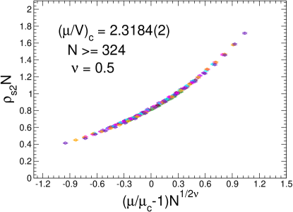
Figure 11: Data collapse of the observable $\rho_{s2}N$ with $18^{2}\leq N\leq 32^{2}$ for the quantum phase transition from a supersolid state to a solid state of $\rho=1/2$. The data is calculated using $\beta=N/4$. In obtaining the figure, the critical exponent $\nu$ is fixed to be the expected theoretical value $\nu=0.5$.

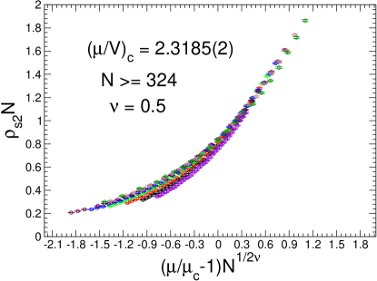
Figure 12: Data collapse of the observable $\rho_{s2}N$ with $18^{2}\leq N\leq 32^{2}$ for the quantum phase transition from a supersolid state to a solid state of $\rho=1/2$. The data is calculated using $\beta=8N^{1/2}$. In obtaining the figure, the critical exponent $\nu$ is fixed to be the expected theoretical value $\nu=0.5$.

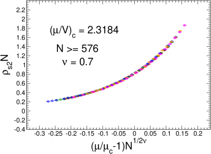
Figure 13: Data collapse of the observable $\rho_{s2}N$ with $24^{2}\leq N\leq 32^{2}$ for the quantum phase transition from a supersolid state to a solid state of $\rho=1/2$. The data is calculated using $\beta=8N^{1/2}$. In obtaining the figure, the critical chemical potential $\mu_{c}$ and the critical exponent $\nu$ are fixed to be $\mu_{c}=2.3184$ and $\nu=0.7$, respectively.

In additional to the quantum phase transition from a supersolid phase to a solid phase of $\rho=1/2$ for the extended Bose-Hubbard model, we have studied the critical theory of the phase transition from a superfluid phase to a Mott insulator phase of $\rho=1$ as well. Inspired by the subtlety we observed earlier, we use $\beta=N/2.5$ for this new investigation since the dynamical critical exponent $z$ for this transition is predicted to be 2 theoretically. Indeed using $\nu=0.5$ which is the expected theoretical value for $\nu$, a good data collapse is reached for $\rho_{s2}N$ provided that $(\mu/V)_{c}=3.6378(2)$ and $N\geq 16^{2}$ (figure 14). In other words, our Monte Carlo data is fully compatible with the predicted universality class for the transition from a superfluid phase to a Mott insulator phase of $\rho=1$.

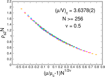
Figure 14: Data collapse of the observable $\rho_{s2}N$ with $18^{2}\leq N\leq 32^{2}$ for the quantum phase transition from a superfluid state to a Mott insulator state of $\rho=1$. The data is calculated using $\beta=N/2.5$. In obtaining the figure, the critical exponent $\nu$ is fixed to be the expected theoretical value $\nu=0.5$.

IV Discussions and Conclusions

In this paper, we use first principles Monte Carlo methods to study the quantum phase transitions from a supersolid phase to a solid phase of $\rho=1/2$ and from a superfluid phase to a Mott insulator phase of $\rho=1$ by varying the chemical potential $\mu/V$ at fixed $U/t=20$ and $t/V=0.16$ in the parameter space for the extended Bose-Hubbard model. We confirm that our Monte Carlo results for both phase transitions are fully compatible with the corresponding theoretical prediction. Specifically, we obtain a good quality of data collapse for $\rho_{s2}N$ with fixed $\nu=0.5$ and $z=2$ in the analysis. On the other hand, we find it is subtle to determine the correct critical chemical potential $(\mu/V)_{c}$ for the phase transition from a supersolid phase to a soild phase of $\rho=1/2$. For example, while the $(\mu/V)_{c}$ calculated from a set of $\rho_{s2}$ data obtained using $\beta=2N^{1/2}$ is given by $(\mu/V)_{c}=2.3289(2)$, another set of $\rho_{s2}$ data determined from the simulations with $\beta=N/2$ leads to $(\mu/V)_{c}=2.3186(2)$. The deviation of these two values of $(\mu/V)_{c}$ found from different strategies of scaling the inverse temperature $\beta$ with the system sizes is statistically significant. The later result for $(\mu/V)_{c}$ should be more reliable considering the fact that the dynamical critical exponent $z$ is 2. We also demonstrate that using the incorrect scaling of $\beta$, namely one scales $\beta$ linearly with the system linear length $N^{1/2}$, would either lead to bad quality of data collapse for the observables considered here, or one would arrive at a different critical theory for the phase transition investigated in this study. Despite the fact that the principles behind the technique of data collapse is exact, it might mislead one to conclude an observation of an unconventional phase transition. Our results of $(\mu/V)_{c}=2.3184$ and $\nu=0.7$ obtained by carrying out the data collapse for $\rho_{s2}N$ determined from the simulations with $\beta=8N^{1/2}$ is a good example of such a scenario. When applying the technique of data collapse to study the critical theory of a second order phase transition, it might be useful to employ this technique in a more rigorous manner. At this stage, it is a surprise that the motivation behind our investigation, namely whether scaling $\beta$ linearly with the system linear length for studying a second order phase transition with $z=2$ is an appropriate strategy, is ignored in some studies of phase diagrams for certain models in the literature. To re-examine the corresponding critical points seems to be the required step in order to confirm the quantitative correctness of the established phase diagrams of some spin and bose models. Our results does not necessarily indicate that the phase diagram of the bilayer spin-1/2 Heisenberg model in an external magnetic field studied in Laf07 and the phase diagram of extended Bose-Hubbard model mapped out in Gan07_2 are not quantitatively correct. However one might need to reconsider the phase diagrams of these models if the precise location of a critical point in the parameter space is crucial in drawing a conclusion. Finally, based on the results presented in this paper, in particular the unexpected $\nu=0.7$ obtained from the data $\rho_{s2}N$ calculated with $\beta=8N^{1/2}$, it will be important to determine the dynamical critical exponent $z$ first when investigating the critical theory for a second order phase transition which might be described by a new universality class and is poor known theoretically.

References

- (1) P. Sengupta et al., Phys. Rev. Lett. 94, 207202 (2005).
- (2) S. Wessel and M. Troyer, Phys. Rev. Lett. 95, 127205 (2005).
- (3) R. Melko et al., Phys. Rev. Lett. 95, 127207 (2005).
- (4) M. Boninsegni and N. Prokof’ev, Phys. Rev. Lett. 95, 237204 (2005).
- (5) R. G. Melko, A. Del Maestro, and A. A. Burkov, Phys. Rev. B 74, 214517 (2006).
- (6) Kwai-kong Ng and T.-K. Lee, Phys. Rev. Lett. 97, 127204 (2006).
- (7) P. Sengupta and C. D. Batista, Phys. Rev. Lett. 98, 227201 (2007).
- (8) Jing Yu Gan, Yu Chuan Wen, and Yue Yu, Phys. Rev. B 75, 094501 (2007).
- (9) S. Wessel, Phys. Rev. B 75, 174301 (2007).
- (10) J. Y. Gan, Y. C. Wen, J. Ye, T. Li, S.-J. Yang, and Y. Yu, Phys. Rev. B 75, 214509 (2007).
- (11) N. Laflorencie and F. Mila, Phys. Rev. Lett. 99, 027202 (2007).
- (12) Yu-Chun Chen, Roger G. Melko, Stefan Wessel, and Ying-Jer Kao Phys. Rev. B 77, 014524 (2008)
- (13) M. Greiner et al., Nature 415, 39 (2002).
- (14) T. Stöferle, et al., Phys. Rev. Lett. 91, 130403 (2004).
- (15) S. Fölling, et al., Phys. Rev. Lett. 97, 060403 (2006).
- (16) M. Batrouni and R. T. Scalettar, Phys. Rev. Lett. 84, 1599 (2000).
- (17) K. S. Novoselov. et al., Science 306, 666 (2004).
- (18) K.S. Novoselov, et al., Nature 438, 197 (2005).
- (19) Y. Zhang, et al., Nature 438, 201 (2005).
- (20) A.H. Castro Neto, F. Guinea, N.M.R. Peres, K.S. Novoselov, and A.K. Geim, Rev. Mod. Phys. 81: 109-162, 2009.
- (21) M .P. A. Fisher et al., Phys. Rev. B 40, 546 (1989).
- (22) F. Alet and E. S. Sorensen, Phys. Rev. B 70, 024513 (2004).
- (23) A. F. Albuquerque et. al, Journal of Magnetism and Magnetic Material 310, 1187 (2007).