$\rm{K}^{0}-\overline{\rm{K}}^{0}$ on the Lattice

Petros Dimopoulos

Physics Department
University of Rome “La Sapienza”
piazz.le Aldo Moro 2, I-00185 Rome, Italy

I review recent lattice calculations performed with $N_{f}=2$ and $N_{f}=2+1$ dynamical fermions which provide a precise computation of the $B_{\rm{K}}$ bag parameter. I also report on $N_{f}=2$ dynamical quark simulations aiming at the computation of the full basis of the $\Delta S=2$ four-fermion operator matrix elements that are relevant to models beyond the Standard Model.

PRESENTED AT

Proceedings of CKM2010,
the 6th International Workshop
on the CKM Unitarity Triangle,
University of Warwick, UK, 6-10 September 2010

1 Introduction

The indirect CP violation, present in the neutral Kaon meson pair ($\rm{K}^{0}-\overline{\rm{K}}^{0}$) oscillations [1], is a confirmed experimental fact. The neutral Kaons ${\rm K}^{0}=(\overline{s}d)$ and $\overline{\rm{K}}^{0}=(s\overline{d})$ are flavour eigenstates which, in the Standard Model (SM), can mix to lowest order through a box diagram due to the weak interactions. The weak hamiltonian describing the time evolution of the kaon pair system can be expressed via a 2 $\times$ 2 non-hermitian matrix, $H=M-i\Gamma/2$. The dispersive and absorptive parts, $M$ and $\Gamma$ respectively, are hermitian matrices. Defining the CP eigenstates $|K_{\pm}\rangle=(|K^{0}\rangle\pm|\overline{K}^{0}\rangle)/\sqrt{2}$, it turns out that the two hamiltonian eigenstates, called $K-$ short and $K-$ long, are $|K_{\scriptstyle{S/L}}\rangle=\frac{\textstyle{1}}{\textstyle{\sqrt{1+\overline{\epsilon}^{2}}}}~{}(|K_{\pm}\rangle+\overline{\epsilon}|K_{\mp}\rangle)$. The paramater $\overline{\epsilon}$ represents the mixing between the two CP eigenstates; it depends on the phase conventions of the eigenstates and represents the theoretical measure of the indirect CP violation. On the other hand the experimental measurement involves a phase independent quantity which is

$$\epsilon_{\rm{K}}=\frac{{\cal A}(K_{L}\longrightarrow(\pi\pi)_{I=0}))}{{\cal A}(K_{S}\longrightarrow(\pi\pi)_{I=0}))}$$ (1)

It turns out that (Ref. [2]) $\epsilon_{\rm{K}}=\overline{\epsilon}+i\xi$, where $\xi=\frac{\textstyle{\rm{Im}\,A_{0}}}{\textstyle{\rm{Re}\,A_{0}}}$ and $A_{0}$ is the isospin zero amplitude for the $\rm{K}^{0}$ decay to either $(\pi^{0}\pi^{0})$ or $(\pi^{-}\pi^{+})$. It has been shown ( [3],[4], [5]; see also [6]) that, under reasonable estimates for the long-distance contribution to both the dispersive and the absorptive parts of the hamiltonian, $\epsilon_{\rm{K}}$ is approximately given

$$\epsilon_{\rm{K}}\simeq\kappa_{\epsilon}\frac{e^{i\phi_{\epsilon}}}{\sqrt{2}}\frac{\rm{Im}\,M_{12}}{\Delta m_{\rm{K}}}$$ (2)

In Eq. (2) the phase $\phi_{\epsilon}=43.51(5)^{o}$ and the mass difference between $\rm{K}_{L}$ and $\rm{K}_{L}$, $\Delta m_{\rm{K}}=3.483(6)\times 10^{-12}~{}\rm{MeV}$, have been determined experimentally with high precision [7]. The factor $\kappa_{\epsilon}=0.94(2)$ incorporates in an approximate way the effect of the long distance contributions mentioned above.

In the SM the calculation of $\rm{Im}\,M_{12}$ is performed in the Operator Product Expansion (OPE) approach. Once the heavy degrees of freedom, including the charm quark, are integrated out the CP violation contribution in the neutral K-meson mixing is described in terms of the $\overline{K}^{0}-K^{0}$ matrix element of a local $\Delta S=2$ four-fermion operator:

$$M_{12}=\frac{1}{2m_{\rm{K}}}(\langle\overline{K}^{0}|{\cal H}_{eff}^{\Delta S=2}|K^{0}\rangle)^{*}=\frac{1}{2m_{\rm{K}}}C_{{\cal W}}^{\rm{SM}}(\mu)(\langle\overline{K}^{0}|{\cal O}^{\Delta S=2}(\mu)|K^{0}\rangle)^{*}$$ (3)

The Wilson coefficient $C_{{\cal W}}^{\rm{SM}}(\mu)$ contains all the short distance effects which are calculated in perturbation theory. The matrix element of the four-fermion operator ${\cal O}^{\Delta S=2}\equiv{\cal O}_{1}=(\overline{s}d)_{V-A}(\overline{s}d)_{V-A}\equiv\overline{s}\gamma_{\mu}(1-\gamma_{5})d\,\,\overline{s}\gamma_{\mu}(1-\gamma_{5})d$ is written in the form

$$\langle\overline{K}^{0}|{\cal O}_{1}(\mu)|K^{0}\rangle=\frac{8}{3}m_{\rm{K}}^{2}f_{\rm{K}}^{2}B_{\rm{K}}(\mu)$$ (4)

where the parameter $B_{\rm{K}}$ is the amount by which it differs from its Vacuum Saturation Approximation (VSA) value and $m_{\rm{K}}$ and $f_{\rm{K}}$ are the mass and the decay constant of the Kaon respectively. Therefore the bag parameter $B_{\rm{K}}$ is the measure of the non-perturbative QCD contribution in the hadronic matrix element of the K-meson pair oscillation. The Renormalisation Group Invariant (RGI) quantity is defined by the equation

$$\hat{B}_{\rm{K}}=\raisebox{-1.29167pt}{\mbox{\LARGE$\left[\right.$}}\alpha_{s}^{(3)}(\mu)\raisebox{-1.29167pt}{\mbox{\LARGE$\left.\right]$}}^{-2/9}~{}\raisebox{-1.29167pt}{\mbox{\LARGE$\left[\right.$}}1+\frac{\alpha_{s}^{(3)}(\mu)}{4\pi}\,J_{3}\raisebox{-1.29167pt}{\mbox{\LARGE$\left.\right]$}}B_{\rm{K}}({\mu})$$ (5)

where $\alpha_{s}^{(3)}(\mu)$ is the running coupling constant for $N_{f}=3$ flavours and $J_{3}$ has been computed up to NLO order [8]. Eqs. (2)-(5) yield

$$|\epsilon_{K}|=\kappa_{\epsilon}C_{\epsilon}\hat{B}_{\rm{K}}\,|V_{cb}|^{2}\lambda^{2}\overline{\eta}\raisebox{-1.29167pt}{\mbox{\LARGE$\left[\right.$}}-\eta_{1}S_{0}(x_{c})(1-\frac{\lambda^{2}}{2})+\eta_{2}S_{0}(x_{t})|V_{cb}|^{2}\lambda^{2}(1-\overline{\rho})+\eta_{3}S_{0}(x_{c},x_{t})\raisebox{-1.29167pt}{\mbox{\LARGE$\left.\right]$}}$$ (6)

where $C_{\epsilon}=\frac{G_{F}^{2}f_{\rm{K}}^{2}m_{\rm{K}}M_{\rm{W}}^{2}}{6\sqrt{2}\pi^{2}\Delta m_{\rm{K}}}$ and $\lambda=|V_{us}|$. $S_{0}$ are the Inami-Lim functions depending on $x_{c,t}=m_{c,t}^{2}/M_{\rm{W}}^{2}$ and give the charm, top and charm-top contributions to the box diagram; $\eta_{i=1,2,3}$ contain the corresponding short distance QCD contributions to NLO order ([9]-[11]). The experimental value of $|\epsilon_{K}|=2.228(11)\times 10^{-3}$ is known with high precision [7]. Therefore, the hyperbola defined by Eq. (6) in the $(\overline{\rho},\overline{\eta})$ plane can be used to (over-)constrain the upper vertex of the unitarity triangle with a precision that depends on the quality of the estimates of $|V_{us}|$, $|V_{cb}|$ and $\hat{B}_{\rm{K}}$. While the numerical value of the first is known to very good precision (see Ref. [13]), the estimate of (inclusive) $|V_{cb}|$ (Ref. [14]) is still given with un uncertainty of $\sim 2\%$ which gets amplified four times in Eq. (6) because it enters to the fourth power. $\hat{B}_{\rm{K}}$ can be calculated on the lattice from first principles. Its estimate, until 2008, used to represent the largest source of uncertainty in Eq. (6) but now, thanks to recent precision lattice calculations, it is known with a total (statistical and systematic) uncertainty of less than $4\%$. This is the consequence of employing unquenched simulations with $N_{f}=2$ and $N_{f}=2+1$ dynamical quarks with high statistics, controlling with better accuracy both the discretization errors and the extrapolation to the physical point and using non-perturbative methods for the renormalisation of the operators on the lattice.

2 $\mathbf{B_{\rm{K}}}$ calculation on the lattice

2.1 General considerations

The evaluation of $B_{\rm{K}}$ on the lattice requires the computation of a three point correlation function with the insertion of two pseudoscalar meson interpolating fields at two time slices, say, $t_{1}$ and $t_{2}$ and the insertion of the $\Delta S=2$ four-fermion operator considered at any time slice $t_{0}$ with $t_{0}\in[t_{1},t_{2}]$. In order to carry out the computation of Eq. (4), the three point correlation function needs to be divided by two two-point correlation functions each of which involves a pseudoscalar meson and an axial current interpolating fields; then one takes the asymptotic limit i.e. $t_{1}\ll t_{0}\ll t_{2}$ in order to obtain the value of the matrix element between the lowest-lying states. In summary, one has

$$\frac{\langle{\cal P}(t_{1})^{\dagger}\,{\cal O}^{\Delta S=2}(t_{0})\,{\cal P}(t_{2})\rangle}{(8/3){\langle\cal P}(t_{1})^{\dagger}{\cal A}_{0}(t_{0})\rangle\,\langle{\cal A}_{0}(t_{0})^{\dagger}{\cal P}(t_{2})\rangle}\xrightarrow{t_{1}\ll t_{0}\ll t_{2}}\frac{\langle{\overline{K}^{0}}|{\cal O}^{\Delta S=2}|{K^{0}}\rangle}{(8/3)\langle\overline{K}^{0}|A_{0}|0\rangle\langle 0|A_{0}^{\dagger}|K^{0}\rangle}=B_{\rm{K}}$$ (7)

where ${\cal P}(t)$ and ${\cal A}(t)$ denote the pseudoscalar density and axial current interpolating fields respectively. Note also that $\langle 0|A_{0}|K^{0}\rangle=f_{\rm{K}}\,m_{\rm{K}}$. In practice, due to parity conservation in QCD, one needs to evaluate only the matrix element of the parity-even part, ${\cal O}_{VV+AA}=\overline{s}\gamma_{\mu}d\overline{s}\gamma_{\mu}d+\overline{s}\gamma_{\mu}\gamma_{5}d\overline{s}\gamma_{\mu}\gamma_{5}d$, of the ${\cal O}^{\Delta S=2}$ operator.

Naturally, a renormalization step is necessary to get finite results in the continuum limit ($a\rightarrow 0$). For this purpose the renormalization constant (RC) of the operator ${\cal O}$, $Z_{{\cal O}}$, (or a full matrix of RCs in the general case where more than one operators get mixed in the renormalisation procedure) has to be computed at a certain scale $\mu$ (the same as that of the Wilson coefficient). Lattice perturbation theory can be used. The result, however, suffers from more or less insufficiently well estimated systematic errors due to the truncation of the perturbative expansion. This is especially true for not so fine lattice spacings. In any case non-perturbative methods offer a more accurate way in computing the RC of operators. By imposing renormalization conditions on correlation functions with operator insertions and performing calculations of matrix elements on the lattice, one has the opportunity to embody in the calculation both higher order contibutions and non-perturbative effects. In this way the remaining sources of systematic error are only due to the use of perturbation theory in passing from the lattice scheme (at some scale $\mu$) to a continuum renormalisation scheme.

Lattice calculations are performed at a number of various values of lattice spacing and suffer from discretization errors which can be eliminated when the extrapolation to the continuum limit (c.l.) is achieved. This source of systematic error can be well kept under control if the values of the lattice spacing are small, typically less than about 0.1 fm. Then simulations for at least three values of the lattice spacing are typically necessary to be able to perform the extrapolation to the continuum limit. In most of the cases discretization error of the various physical quantities measured on the lattice are of at most $O(a^{2})$.

It is interesting to have a look at the “world-average” values of $\hat{B}_{\rm{K}}$ which cover a period of the past fifteen years as they reported at the Lattice Conferences. The RGI results (computed with the same running using $N_{f}=3$ flavours, see Ref. [15]) are shown in Fig. 1.

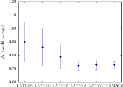
Figure 1: $\hat{B}_{\rm{K}}$ “world averages” over the last fifteen years reported at the Lattice Conferences. The world average result at CKM2010 is also included.

It is impressive to notice the great improvement in the quality of the results where total uncertainty has decreased by almost five times in the last fifteen years. It should also be noticed that even until 2005 the $\hat{B}_{\rm{K}}$ “world average” result was based on estimates computed in the quenched approximation with the systematic error due to quenching being in practice unknown. However, the “world average” value of the last two years is based only on results produced with unquenched simulations.

2.2 Recent lattice $\mathbf{B_{\rm{K}}}$ computations

Different lattice groups compute $B_{\rm{K}}$ using a variety of lattice regularizations which conserve (most of) the chiral symmetry and provide well controlled and small $O(a^{2})$ discretization errors. Besides that, simulations have been performed at a well tuned physical value for the strange quark mass while the lightest simulated quark mass value, even if not yet at its physical value, has smaller values than in any preceding calculation of $B_{\rm{K}}$. Four collaborations, performing unquenched simulations, have computed the continuum limit value for $B_{\rm{K}}$. Three of them have simulated $N_{f}=2+1$ dynamical quarks, while the fourth one has used $N_{f}=2$ dynamical quark simulations.

Collaboration	$N_{f}$	fermion discr.	$a\,[\rm{fm}]$	$\raisebox{-1.29167pt}{\mbox{\LARGE$\left[\right.$}}M_{\pi}^{\rm{val}}/M_{\pi}^{\rm{sea}}\raisebox{-1.29167pt}{\mbox{\LARGE$\left.\right]$}}_{\rm{min}}$	$\raisebox{-1.29167pt}{\mbox{\LARGE$\left[\right.$}}M_{\pi}^{\rm{val}}L\raisebox{-1.29167pt}{\mbox{\LARGE$\left.\right]$}}_{\rm{min}}$	Renorm/tion
		val. / sea		in [MeV]
ALV                [16]	2+1	DW/Asqtad	0.12, 0.09	240/370	3.5	Non-Pert.
BSW               [17]	2+1	HYP-stag/Asqtad	0.12, 0.09, 0.06	240/300	2.5	Pert.
RBC-UKQCD [18]	2+1	DW/DW	0.11, 0.09	220/290	3.1	Non-Pert.
ETMC             [19]	2	OS/TM	0.10, 0.09, 0.07	280/280	3.3	Non-Pert.

Table 1: Simulation details of unquenched simulations of $B_{\rm{K}}$ computation with $N_{f}=2$ and $N_{f}=2+1$ dynamical quarks.

Table 1 gives a summary of the simulation details for the computation by each collaboration; Table 2 contains $B_{\rm{K}}$ results expressed in the $\overline{\rm{MS}}$ scheme at 2 GeV as well as in the RGI definition (see Refs. [16]-[19]); the first error is statistical while the second is the systematic one; the total error has to be calculated as the sum in quadrature of the statistical and the systematic ones. In the following paragraphs a short description of each computation is presented.

Aubin, Laiho and Van de Water (ALV) (see Ref. [16]) have presented a mixed action calculation performed with Domain Wall (DW) fermion regularization in the valence quark sector on $N_{f}=2+1$ dynamical Asqtad-improved staggered quarks (MILC). DW fermions in the valence sector offer the possibility to use the MILC dynamical configurations without having to bother about taste mixing. Since they have a residual chiral breaking (due to the finite size of the fifth lattice dimension), the renormalisation of the parity even four-fermion operator suffers from mixing with operators of wrong chirality through coefficients whose values are expected to be suppressed at order $O((am_{res})^{2})$. The implementation of the non-perturbative renormalisation method (RI-MOM) is straightforward for DW fermions. They have done simulations at two values of lattice spacing, namely $a=0.12$ and $0.09$ fm. They extrapolate to the physical point using fit functions based on Mixed action $\chi$PT with the addition of NNLO analytical terms. Their result is given in Table 2 ; a large part of the systematic error quoted is due to the uncertainty in the renormalisation constant computation.

Bae et al. (BSW, see Ref. [17]) have also completed a mixed action computation where they have used HYP-smeared staggered valence quarks on MILC $2+1$ dynamical quark configurations. The choice for this particular valence quark regularization is justified by its property of dispalying rather small taste breaking effects and a computationally cheap implementation. They extrapolate to the physical point trying fit functions based on SU(3) and SU(2) Staggered-$\chi$PT. The two fitting procedures give compatible results with the latter being more straightforward in fitting the data. Simulations have been carried out at three values of lattice spacing, $a=0.12$, 0.09 and 0.06 fm. The dominant source of uncertainty is due to the perturbative approach they use to renormalize the four-fermion operator. In fact, the total error is almost $6\%$ the larger part of which is due to RC’s uncertainty.

RBC-UKQCD Collaboration (Ref. [18]) used a $N_{f}=2+1$ DW action both for the sea and the valence quarks at two values of the lattice spacing, $a=0.11$ and 0.09 fm. The renormalization of the four-fermion operator is performed employing RI-MOM methods where non-exceptional momentum renormalization conditions and twisted boundary conditions have been applied. They achieve further suppression of the residual wrong chirality mixing and a matching to $\overline{\rm{MS}}$ at a higher scale value (3 GeV) which allows for a a better control of the perturbative systematic uncertainty. The uncertainty to the final value due to the renormalisation procedure is estimated 2$\%$. The physical point is reached via a combined continuum and SU(2) PQ$\chi$PT fitting formula. The total error in the final value is $3.6\%$, while the pure stastistical one is about $0.9\%$.

ETM Collaboration (Ref. [19]) has adopted a mixed action set-up to perform the computation with a Wilson fermion regularization. Actually, since Wilson fermions explicitly break the chiral symmetry, the relevant $B_{\rm{K}}$ computation done with the use of plain Wilson quarks suffers from $O(a)$ discretization errors and yields wrong chirality mixing in the process of renornalizing the lattice ${\cal O}_{VV+AA}$ operator. It is known that both problems can inject serious systematic uncertainties in the computation. However, it has been shown that they can be tackled simultaneously by employing Osterwalder-Seiler (OS) valence on Twisted Mass (TM) sea fermions, both tuned at maximal twist (see Ref. [20]). ETMC has carried out the computation working with $N_{f}=2$ dynamical quark simulations, so the strange quark is still quenched. Unitarity violations due to the mixed action set-up, that are expected to be $O(a^{2})$ effects, have been shown to be well under control in the continuum limit. The extrapolation to the physical light quark mass is performed using a fit function based on SU(2)-$\chi$PT while three values of the lattice spacing, $a=0.10$, 0.09 and 0.07 fm, have been used to extrapolate to the continuum limit. The renormalization of the four-fermion operator has been carried out in a non-perturbative way using the RI-MOM method. The mixing with operators of wrong chirality has been shown to be numerically negligible. The total error is $4\%$.

Collaboration		$N_{f}$	$B_{\rm{K}}^{\overline{\rm{MS}}}(2\,\rm{GeV})$	$\hat{B}_{\rm{K}}$
ALV	[16]	2+1	0.527(06)(20)	0.724(08)(28)
BSW	[17]	2+1	0.529(09)(32)	0.724(12)(43)
RBC-UKQCD	[18]	2+1	0.549(05)(26)	0.749(07)(26)
ETMC	[19]	2	0.517(18)(11)	0.729(25)(17)

Table 2: Results in the continuum limit for the $B_{\rm{K}}$-parameter expressed in the $\overline{\rm{MS}}$ scheme and in the RGI definition from unquenched simulations with $N_{f}=2$ and $2+1$ dynamical quarks. The first error is quoted as statistical while the second is the estimate of the systematic uncertainties.

The $\hat{B}_{\rm{K}}$ results published in the last five years and computed on quenched ($N_{f}=0$) and unquenched lattices with $N_{f}=2$ and $N_{f}=2+1$ dynamical quark simulations are collected in Fig. 2. The label (c.l.) is attached to the $\hat{B}_{\rm{K}}$ values obtained after the continuum limit has been taken. Vertical lines indicate the average $\hat{B}_{\rm{K}}$ result with its error, based on $N_{f}=2+1$ simulations, which is

$$\hat{B}_{\rm{K}}=0.736(05)(26)~{}~{}~{}~{}@~{}~{}~{}~{}N_{f}=2+1$$ (8)

This value has been obtained by taking the average of the $N_{f}=2+1$ results weighted with the quoted statistical error. The systematic uncertainty is the smallest error quoted in Table 2. The total uncertainty is about $3.6\%$. The $\hat{B}_{\rm{K}}$ average for the $N_{f}=2$ case obviously coincides with the result provided by ETMC, since it is the only continuum limit result available. One finds

$$\hat{B}_{\rm{K}}=0.729(25)(16)~{}~{}~{}~{}@~{}~{}~{}~{}N_{f}=2$$ (9)

Results from Eqs. (8) and (9) indicate that the systematic uncertainty due to the quenching of the strange quark has an impact which is smaller than other systematic errors. Moreover, comparing the result of Eq. (8) with the most precise of the quenched results (see Ref. [25]), one can infer that the systematic uncertainty due to the quenching is small (actually $\sim 6\%$).

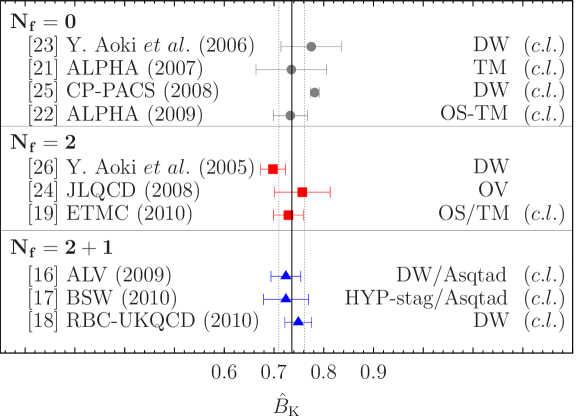
Figure 2: $\hat{B}_{\rm{K}}$ results from $N_{f}$ = 0 (quenched) and unquenched simulations with $N_{f}$ = 2 and $N_{f}$ = 2+1 dynamical quarks. Computations where the continuum limit has been taken are indicated with “(c.l.)”. Vertical lines refer to the average result of Eq. (8). In the plot, results from pioneer works with $N_{f}$ = 2 [27] and $N_{f}$ = 2+1 [28] unquenched simulations have not been included since their quoted total uncertainty is now considered too large compared to today standards.

3 $\mathbf{K^{0}-\overline{K}^{0}}$mixing beyond the SM

There are various models for the physics Beyond the SM (BSM) which lead to other possible $\Delta S=2$ processes at one loop. In this case the computation of the relevant matrix elements of the effective hamiltonian in combination with the experimental value of $\epsilon_{\rm{K}}$ would offer the chance of obtaining constraints on the parameters of the model (like for instance estimates on the off-diagonal terms of the squark matrix in supersymmetric models [29]) which enter explicitly in the Wilson coefficients.

The general form for the $\Delta S=2$ effective Hamiltonian in BSM models reads

$${\cal H}_{\rm{eff}}^{\Delta S=2}=\sum_{i=1}^{5}C_{i}(\mu){\cal O}_{i}+\sum_{i=1}^{3}\tilde{C}_{i}(\mu)\tilde{{\cal O}}_{i}$$ (10)

where

$${\cal O}_{1} = [\overline{s}^{a}\gamma_{\mu}(1-\gamma_{5})d^{a}][\overline{s}^{b}\gamma_{\mu}(1-\gamma_{5})d^{b}],$$

$${\cal O}_{2} = [\overline{s}^{a}(1-\gamma_{5})d^{a}][\overline{s}^{b}(1-\gamma_{5})d^{b}],~{}~{}~{}~{}~{}~{}~{}~{}{\cal O}_{3}=[\overline{s}^{a}(1-\gamma_{5})d^{b}][\overline{s}^{b}(1-\gamma_{5})d^{a}],$$

$${\cal O}_{4} = [\overline{s}^{a}(1-\gamma_{5})d^{a}][\overline{s}^{b}(1+\gamma_{5})d^{b}],~{}~{}~{}~{}~{}~{}~{}~{}{\cal O}_{5}=[\overline{s}^{a}(1-\gamma_{5})d^{b}][\overline{s}^{b}(1+\gamma_{5})d^{a}]$$

$$\tilde{{\cal O}}_{1} = [\overline{s}^{a}\gamma_{\mu}(1+\gamma_{5})d^{a}][\overline{s}^{b}\gamma_{\mu}(1+\gamma_{5})d^{b}],$$

$$\tilde{{\cal O}}_{2} = [\overline{s}^{a}(1+\gamma_{5})d^{a}][\overline{s}^{b}(1+\gamma_{5})d^{b}],~{}~{}~{}~{}~{}~{}~{}~{}\tilde{{\cal O}}_{3}=[\overline{s}^{a}(1+\gamma_{5})d^{b}][\overline{s}^{b}(1+\gamma_{5})d^{a}]$$ (11)

We have seen that in the SM case, Eq. (3), only the operator ${\cal O}_{1}$ contributes.
The parity-even parts of the operators $\tilde{{\cal O}}_{i}$ coincide with those of the operators ${\cal O}_{i}$. Therefore, due to parity conservation in the strong interactions only the parity-even contribution of the operators ${\cal O}_{i}$ need to be calculated. A basis of the parity-even operators is

$$O^{VV} = (\overline{s}\gamma_{\mu}d)(\overline{s}\gamma_{\mu}d),~{}~{}~{}~{}~{}~{}~{}~{}O^{AA}=(\overline{s}\gamma_{\mu}\gamma_{5}d)(\overline{s}\gamma_{\mu}\gamma_{5}d),$$

$$O^{PP} = (\overline{s}\gamma_{5}d)(\overline{s}\gamma_{5}d),~{}~{}~{}~{}~{}~{}~{}~{}~{}O^{SS}=(\overline{s}d)(\overline{s}d),$$

$$O^{TT} = (\overline{s}\sigma_{\mu\nu}d)(\overline{s}\sigma_{\mu\nu}d)$$ (12)

in terms of which and after using a Fierz transformation one obtains the relations

$${\cal O}_{1} = (O^{VV}+O^{AA}),~{}~{}~{}~{}{\cal O}_{2}=(O^{SS}+O^{PP}),~{}~{}~{}~{}{\cal O}_{3}=-\frac{1}{2}(O^{SS}+O^{PP}-O^{TT}),$$

$${\cal O}_{4} = (O^{SS}-O^{PP}),~{}~{}~{}~{}~{}{\cal O}_{5}=-\frac{1}{2}(O^{VV}-O^{AA})$$ (13)

The B-parameters for the operators of Eq. (3) are defined as

$$\langle\overline{K}^{0}|{\cal O}_{1}(\mu)|K^{0}\rangle = B_{1}(\mu)\frac{8}{3}m_{K}^{2}f_{K}^{2}\equiv B_{K}(\mu)\frac{8}{3}m_{K}^{2}f_{K}^{2}$$

$$\langle\overline{K}^{0}|{\cal O}_{i}(\mu)|K^{0}\rangle = C_{i}B_{i}(\mu)\raisebox{-1.29167pt}{\mbox{\LARGE$\left[\right.$}}\frac{m_{K}^{2}f_{K}}{m_{s}(\mu)+m_{d}(\mu)}\raisebox{-1.29167pt}{\mbox{\LARGE$\left.\right]$}}^{2},$$

where $C_{i}=\{-5/3,1/3,2,2/3\},~{}~{}i=2,\ldots,5$. The matrix element of the operator ${\cal O}_{1}$ vanishes in the chiral limit while the matrix element of the operators ${\cal O}_{i},~{}i=2,\ldots,5$ get a non-zero value in the chiral limit. From the above equations it can be seen that the calculation of the $B_{i}$ parameters for $i=2,\ldots,5$ involves the calculation of the quark mass at a common renormalization scale $\mu$. In order to avoid any extra systematic uncertainties in the computation of the matrix elements due to the quark mass evaluation, an alternative calculation has been proposed which consists in calculating directly appropriate ratios of the ${\cal O}_{i},~{}i=2,\ldots,5$ four-fermion matrix elements with the ${\cal O}_{1}$ one ([30], [31]).

There are a few quenched lattice calculations performed with the use of tree-level improved Wilson fermions [30], overlap fermions [31] and DW fermions [32]. However only the first two computations have been carried out using two values of the lattice spacing allowing for the possibility of estimating discretisation effects. A preliminary study referring to the bare matrix elements computation using $N_{f}=2+1$ dynamical DW fermions was also presented in Ref. [33]. Recently ETMC has presented a $N_{f}=2$ unquenched calculation using the mixed action set-up described above (Section 2.2). Both $B_{i}$-bag parameters and matrix elements ratios have been calculated at three values of the lattice spacing, $a=0.1$, 0.09 and 0.07 fm from which reliable continuum limit estimates can be obtained. The results presented in Ref. [34] are preliminary; however, it might be useful to proceed at a first comparison between the quenched and the unquenched estimates for the bag-parameters $B_{i},~{}i=2,\ldots,5$ calculated in the $\overline{\rm{MS}}$ scheme at 2 GeV. This comparison is provided in Fig. 3.

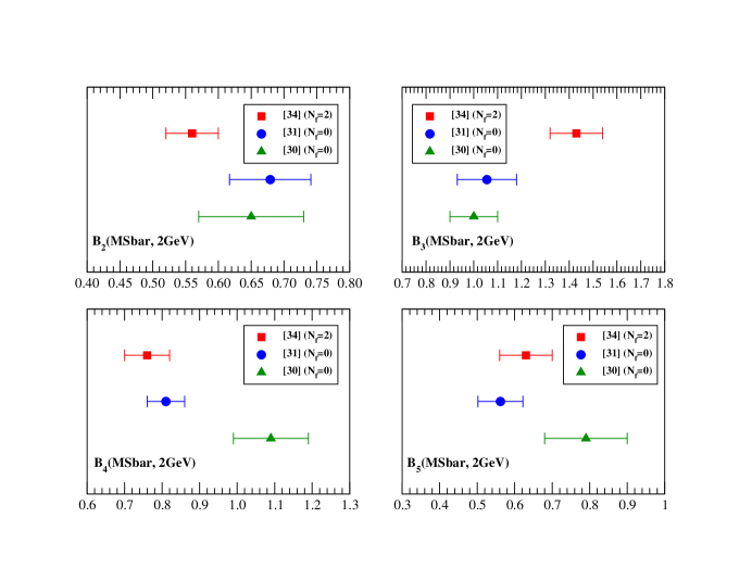
Figure 3: Comparison of continuum limit $B_{i},~{}(i=2,\ldots,5)$ results (in $\overline{\rm{MS}}$ scheme at 2 GeV) obtained using $N_{f}$ = 0 (quenched) ([30], [31]) and unquenched $N_{f}$ = 2 simulations [34].

4 Conclusions

$B_{\rm{K}}$ computation on the lattice has already entered the era of precision measurements with fully unquenched simulations. A number of lattice collaborations using various lattice regularizations provide results that are in nice agreement among themselves. The total estimated uncertainty is less than $4\%$; as a consequence the lattice calculations are not responsible any more for the main source of uncertainty in the $\epsilon_{\rm{K}}$ equation (Eq. 6). The comparison of $B_{\rm{K}}$ results produced with $N_{f}=2+1$ and $N_{f}=2$ unquenched simulations indicate that the systematic error due to the quenching of the strange quark is smaller than other systematic uncertianties. The variety of fermion regularisations, today in use, offer a very good control over the contamination of wrong chirality operator mixing in the renormalisation of the $\Delta S=2$ four-fermion operator. Multiplicative renormalization is guaranteed with discretization errors of $O(a^{2})$. Many collaborations use non-perturbative methods for the operator renormalization leading to a good control over an important source of systematic uncertainty. However the operator renormalisation still representes about half of the systematic uncertainties. Another source of systematic error comes from the fit extrapolation to the physical point; both the choice of the fitting function and the relatively large value of the lightest quark mass actually used in the simulations for $B_{\rm{K}}$ inevitably inject a non-negligible systematic uncertainty into the final result. Of course simulations at finer lattice spacing in the near future would make smaller the systematics due to lattice artifacts making more reliable the continuum limit extrapolation itself as well as the evaluation of renormalization constants.

Recently a $N_{f}=2$ unquenched computation of the matrix elements of the full $\Delta S=2$ operator basis emerging from box diagrams in models beyond the Standard Model has been presented by the ETM Collaboration using three values of the lattice spacing. The continuum limit extrapolated results offer the opportunity of providing constraints on the input parameters of a class of models BSM.

ACKNOWLEDGEMENTS

I thank the CKM2010 Organiser Committee for the hospitality and financial support. I wish to thank V. Lubicz and G.C. Rossi for carefully reading the manuscript and helpful comments. Discussions with G. Martinelli and F. Mescia are gratefully acknowledged.

References

- [1] J. H. Christenson, J. W. Cronin, V. L. Fitch and R. Turlay, Phys. Rev. Lett. 13 (1964) 138.
- [2] L. L. Chau, Phys. Rept. 95 (1983) 1.
- [3] A. J. Buras and D. Guadagnoli, Phys. Rev. D 78 (2008) 033005 [arXiv:0805.3887 [hep-ph]].
- [4] A. J. Buras, D. Guadagnoli and G. Isidori, Phys. Lett. B 688 (2010) 309 [arXiv:1002.3612 [hep-ph]].
- [5] A. Lenz et al., arXiv:1008.1593 [hep-ph].
- [6] D. Guadagnoli, CKM2010 (proceedings).
- [7] K. Nakamura et al. [Particle Data Group], J. Phys. G 37 (2010) 075021.
- [8] M. Ciuchini et al. Nucl. Phys. B 523 (1998) 501 [arXiv:hep-ph/9711402].
- [9] A. J. Buras, M. Jamin and P. H. Weisz, Nucl. Phys. B 347 (1990) 491.
- [10] S. Herrlich and U. Nierste, Nucl. Phys. B 419 (1994) 292 [arXiv:hep-ph/9310311].
- [11] S. Herrlich and U. Nierste, Nucl. Phys. B 476 (1996) 27 [arXiv:hep-ph/9604330].
- [12] J. Brod and M. Gorbahn, Phys. Rev. D 82 (2010) 094026 arXiv:1007.0684 [hep-ph].
- [13] G. Colangelo et al., [FLAG] [arXiv:1011.4408 [hep-lat]].
- [14] [The Heavy Flavor Averaging Group] D. Asner et al., arXiv:1010.1589 [hep-ex].
- [15] V. Lubicz, PoS LAT2009 (2009) 013 [arXiv:1004.3473 [hep-lat]].
- [16] C. Aubin, J. Laiho and R. S. Van de Water, Phys. Rev. D 81 (2010) 014507 [arXiv:0905.3947 [hep-lat]].
- [17] T. Bae et al., Phys. Rev. D 82 (2010) 114509 [arXiv:1008.5179 [hep-lat]].
- [18] [RBC-UKQCD] Y. Aoki et al., [arXiv:1012.4178 [hep-lat]].
- [19] M. Constantinou et al. [ETM Collaboration], arXiv:1009.5606 [hep-lat].
- [20] R. Frezzotti and G. C. Rossi, JHEP 0410 (2004) 070 [arXiv:hep-lat/0407002].
- [21] ALPHA Collaboration, P. Dimopoulos et al., Nucl. Phys. B 776 (2007) 258 [arXiv:hep-lat/0702017].
- [22] ALPHA Collaboration, P. Dimopoulos, H. Simma and A. Vladikas, JHEP 0907 (2009) 007 [arXiv:0902.1074 [hep-lat]].
- [23] Y. Aoki et al., Phys. Rev. D 73 (2006) 094507 [arXiv:hep-lat/0508011].
- [24] S. Aoki et al. [JLQCD Collaboration], Phys. Rev. D 77 (2008) 094503 [arXiv:0801.4186 [hep-lat]].
- [25] Y. Nakamura, S. Aoki, Y. Taniguchi and T. Yoshie [CP-PACS Collaboration], Phys. Rev. D 78 (2008) 034502 [arXiv:0803.2569 [hep-lat]].
- [26] Y. Aoki et al., Phys. Rev. D 72 (2005) 114505 [arXiv:hep-lat/0411006].
- [27] J. M. Flynn, F. Mescia and A. S. B. Tariq [UKQCD Collaboration], JHEP 0411 (2004) 049 [arXiv:hep-lat/0406013].
- [28] E. Gamiz et al. [HPQCD Collaboration and UKQCD Collaboration], Phys. Rev. D 73 (2006) 114502 [arXiv:hep-lat/0603023].
- [29] M. Ciuchini et al. JHEP 9810 (1998) 008 [arXiv:hep-ph/9808328].
- [30] A. Donini, V. Gimenez, L. Giusti and G. Martinelli, Phys. Lett. B 470 (1999) 233 [arXiv:hep-lat/9910017].
- [31] R. Babich et al. Phys. Rev. D 74 (2006) 073009 [arXiv:hep-lat/0605016].
- [32] Y. Nakamura et al. PoS LAT2006 (2006) 089 [arXiv:hep-lat/0610075].
- [33] J. Wennekers [RBC Collaboration and QKQCD Collaboration], PoS LATTICE2008 (2008) 269 [arXiv:0810.1841 [hep-lat]].
- [34] P. Dimopoulos et al. [ETM Collaboration] PoS(Lattice 2010)302 [arXiv:1012.3355 [hep-lat]].