Introduction to Sporadic Groups

Introduction to Sporadic Groups

Luis J. BOYA

L.J. Boya

Departamento de Física Teórica, Universidad de Zaragoza, 50009 Zaragoza, Spain luisjo@unizar.es

Received September 18, 2010, in final form January 12, 2011; Published online January 16, 2011

This is an introduction to finite simple groups, in particular sporadic groups, intended for physicists. After a short review of group theory, we enumerate the $1+1+16=18$ families of finite simple groups, as an introduction to the sporadic groups. These are described next, in three levels of increasing complexity, plus the six isolated “pariah” groups. The (old) five Mathieu groups make up the first, smallest order level. The seven groups related to the Leech lattice, including the three Conway groups, constitute the second level. The third and highest level contains the Monster group $\mathbb{M}$, plus seven other related groups. Next a brief mention is made of the remaining six pariah groups, thus completing the $5+7+8+6=26$ sporadic groups. The review ends up with a brief discussion of a few of physical applications of finite groups in physics, including a couple of recent examples which use sporadic groups.

group theory; finite groups

20D08; 20F99

1 Introduction

1.1 Motivation

Finite groups were first applied in physics to classify crystals (Bravais); with the advent of quantum mechanics (1925), emphasis shifted towards continuous (Lie) groups (Wigner, Weyl). Around 1960 some groups, like ${\rm SU}(3)$ (flavour) were employed to classify particle states (Gell-Mann). Today one needs no justification to use routinely Lie groups and their representations in physics.

On the other hand, the use of discrete, finite groups in particle physics has been limited to the symmetric group ${\rm S}_{n}$ (statistics for identical particles), and to some involutory operations like CPT. Recently, however, the use of finite groups in particle physics has been rekindled, due to new developments; for example, the Monster group $\mathbb{M}$, which is the largest sporadic group, first defined (ca. 1980) as automorphism group of a certain algebra, was afterwards also built up (around 1984) with the use of vertex operators, a construct typical of the physical super string theory. A Japanese group (Eguchi et al., June 2010) has found relations of the K3 (complex) surface, much used in compactification of extra dimensions, with the Mathieu group ${\rm M}_{24}$, the last of the five groups constituting the first level of the sporadic groups.

So the aim of this review is to introduce finite simple groups, in particular sporadic groups, to a physics audience. We anticipate that the use of these finite groups in physics is only expected to increase, so at this time an introduction to the subject seems justified. In this section we set the stage for the situation, by recalling definitions and elementary properties of our objects, the groups whose order is finite. A nice historical review of groups in physics can be found in [2].

1.2 Elementary definitions and properties

We recall a group $G$ is a set with an internal operation $G\times G\rightarrow G$ ($\{g,k\}\rightarrow gk$) associative with unity $I$ (or Id) and inverse $g^{-1}$. $|G|=n$ denotes the number of elements, the order of the group. If $gk=kg$, the group is called Abelian. Among the infinite ($n=\infty$) groups, Lie groups enjoy a special position, as they can be expressed by a finite number of parameters (real numbers), the dimension of the underlying group manifold: e.g. the rotation group ${\rm SO}(3)$ is a continuous Lie group with three (bounded) parameters [3].

A morphism (homomorphism) $\mu:G\rightarrow Q$ is the natural map, obeying $\mu(gk)=\mu(g)\mu(k)$, for any $g,k\in G$. A subgroup $H\subset G$ is a subset which is group by itself. Conjugation of $g$ by $h$, i.e., $h:g\rightarrow h\cdot g\cdot h^{-1}$ is morphism; it splits $G$ into disjoint classes of conjugate elements. A subgroup $H\subset G$ invariant under conjugation, $gHg^{-1}=H$, is called a normal subgroup (invariant, distinguished); if $A$ is Abelian, any subgroup is normal. A group $G$ is simple, if the only normal subgroups are $G$ itself and the identity $I$. We are interested in finite simple groups:

$$G\ {\rm f\/inite\;simple}\Longleftrightarrow|G|<\infty,\quad{\rm and}\quad H\subset G\ {\rm normal}\ \Longrightarrow\ H=G\quad\mbox{or}\quad H={\rm Id}.$$

The period of $g\in G$ is the minimum $r$ with $g^{r}=I$; period 2 elements are called involutions, $a=a^{-1}$. If $g$ is of period $m$, it and its powers generate the cyclic group $Z_{m}$, Abelian and of order $m$. All even-order groups have involutions a (Cauchy) (pair $g\neq a$ with $g^{-1}:{\rm Id}$ and involutions a form an even-order set). With a pair $H\subset G$, if we form $gH$ for $G\ni g\notin H$, we have the left coset due to $g$; two such, $gH$ and $kH$, verify $|gH|=|kH|=|H|$, so $G$ can be put as union of same-order cosets; similarly for right cosets. Hence, the order of $H$ divides that of $G$: Lagrange theorem; for a prime $p$, the group $Z_{p}$ is therefore simple: it is the first family of finite simple groups, and the only Abelian one. The number of cosets is called the index of $H$ in $G$, written $[G:H]$. $gH\equiv Hg$ if $H\subset G$ is normal; one can then also multiply cosets, forming the so-called quotient group, noted $Q:=G/H$, of order the index, $|Q|=[G:H]$. Viceversa, in any morphism $\mu:G\rightarrow Q$, the image $\mu(G)$ is a subgroup of $Q$, and ${\rm Ker}\,\mu:=\mu^{-1}({\rm Id}_{Q})$ is a normal subgroup of $G$. We write $Q:=G/H$ as a short exact sequence

$$1\longrightarrow H\longrightarrow G\longrightarrow Q\longrightarrow 1,$$

meaning $H$ injects in $G$ (monomorphism), $G$ covers $Q$ (epimorphism) and exactness means e.g. the kernel $(H)$ in the map $G\rightarrow Q$ is the image of previous map, $H\rightarrow G$.

If $z$ in $G$ verifies $g\cdot z\cdot g^{-1}=z$, i.e. is fixed by conjugation, is called central; $I={\rm Id}$ is central; centrals are class by themselves. The set of central elements makes up a normal subgroup, called the centre (center) of the group, noted $C_{G}$. ${\rm SU}(2)$, used as quantum mechanical rotation group, has center $\pm I$, i.e., isomorphic to $Z_{2}$.

If $\mu:G\rightarrow G^{\prime}$ is one-to-one onto, it has an inverse ($\exists\,\mu^{-1}$), and is called isomorphism; groups related by isomorphism are not considered different, $G\approxeq G^{\prime}$. Endomorphism is a $\mu:G\rightarrow G$; the set of endomorphisms of an Abelian group $A$ forms a ring, ${\rm End}(A)$. An isomorphism $i:G\rightarrow G$ is called automorphism, and their set ${\rm Aut}(G)$ is a well defined group for any group $G$. Conjugation is an automorphism, called inner. They form a normal subgroup, ${\rm Inn}(G)$ normal in ${\rm Aut}(G)$, and the quotient ${\rm Aut}(G)/{\rm Inn}(G):={\rm Out}(G)$ is called the group of classes of automorphisms. The natural map $G\rightarrow G$ given by conjugation is morphism, whose kernel is clearly the centre $C_{G}$ of the group. We summarize these definitions in the following diagram $(G^{\prime},{\rm Ab}(G)$ explained next):

$$\begin{array}[]{@{}ccccccc}&&C_{G}&&&&\\ &&\downarrow&&&&\\ G^{\prime}&\rightarrow&G&\rightarrow&{\rm Ab}(G)&&\\ &&\downarrow&&&&\\ &&{\rm Inn}(G)&\rightarrow&{\rm Aut}(G)&\rightarrow&{\rm Out}(G)\end{array}\qquad\qquad{\bf Diagram\ I}$$

The commutator of two elements $g$, $k$ is $g\cdot k\cdot g^{-1}\cdot k^{-1}$, $={\rm Id}$ iff $g$ and $k$ commute, $gk=kg$; all commutators $\{g\cdot k\cdot g^{-1}\cdot k^{-1}\}$ generate a normal subgroup of $G$, called the commutator or derived group, $G^{\prime}$; the quotient $G/G^{\prime}$ is Abelian (as the kernel has “all” noncommutativity), and it is the maximal Abelian image of $G$, called ${\rm Ab}(G)$. If $G=G^{\prime}$ the group is called “perfect”.

$H$ normal in $G$ is maximal, if there is no $K$ normal in $G$ with $H$ normal in $K$; the quotient $G/H$ is then simple, say $Q_{1}$. Now if $S$ is normal maximal in $H$, $Q_{2}:=H/S$ is simple again, etc. For any finite group G the chain of simple quotient $\{Q_{i}\}$ ends in ${\rm Id}$, when the last maximal normal subgroup is already simple. The Jordan–Hölder theorem asserts that the chain $\{Q_{i}\}$ is unique up to the order: it does not depend on the (in general, non-unique) maximal normal subgroup chosen each time. If the family $\{Q_{i}\}$ is Abelian (hence of the form $Z_{p}$), the group $G$ is called solvable. For the opposite case, if $G$ is simple the J-H chain is $\{G,{\rm Id}\}$.

For $K$, $G$ groups, in the set of the Cartesian product $K\times G$ one establishes a group composition law by $(k,g)\cdot(k^{\prime},g^{\prime})=(k\cdot k^{\prime},g\cdot g^{\prime})$, called the direct product. For two groups $K$, $Q$ and a morphism $\mu:Q\rightarrow{\rm Aut}(K)$, one defines the $\mu$-semidirect product, written $K\odot Q$, or $K\otimes_{\mu}Q$ by setting, in the Cartesian product set, the group law related to the morphism: $(k,g)\cdot(k^{\prime},g^{\prime})=(kk^{\prime\prime},gg^{\prime})$, where the aut $\mu(g)$ leads $k^{\prime}$ to $\mu(g)k^{\prime}:=k^{\prime\prime}$.

For a set of $n$ symbols: $1,2,3,\dots,n$, a permutation is a new order $(123\dots n)\rightarrow(1^{\prime}2^{\prime}3^{\prime}\dots n^{\prime})$; their totality makes up the symmetric group ${\rm Sym}_{n}={\rm S}_{n}$, with $n!$ elements; it is said of degree $n$. A transposition (12) is a 2-cycle, e.g. $123\dots n\rightarrow 213\dots n$; any element in ${\rm S}_{n}$ can be written as a product of commutative non-overlapping cycles, e.g. $(12345678)\rightarrow(21453687)$ is written as $(12)(345)(6)(78)$, and this cycle structure is invariant under inner autos (conjugation), so it separates ${\rm S}_{n}$ into its classes, as many as partitions of number $n$; for example, ${\rm S}_{3}$ has three classes, $({\rm Id})=(1)(2)(3)$, $(12)(3)$ and $(123)$; ${\rm S}_{5}$ has ${\rm Part}(5)=7$ classes, etc. Any permutation is reached from ${\rm Id}$ by certain number of transpositions, whose parity (number mod 2) is conjugation invariant: hence, the even permutations, $n!/2$ in number, make up the index-two subgroup ${\rm Alt}_{n}$, necessarily normal (a single coset) with quotient ${\rm S}_{n}/{\rm Alt}_{n}=Z_{2}$. The symmetric group is the most important of the finite groups; an easy theorem of Cayley assures that any group of order $n$ can be seen as subgroup of a certain ${\rm S}_{n}$.

An extension $G$ of $K$ (kernel) by $Q$ (quotient) is the triple (exact sequence) $e$: $1\rightarrow K\rightarrow G\rightarrow Q\rightarrow 1$ or simply $G/K\equiv Q$. All finite groups are so constructed, starting with $K$ and $Q$ simple. Extensions $E$ of $G$ by a cyclic group $Z_{n}$, $E/G\equiv Z_{n}$, are marked at times as $G\cdot n$. Viceversa, coverings (or Schur coverings) are extensions $F$ of a certain $Z_{m}$ by $G$, $F/Z_{m}\equiv G$ and are noted $m\cdot G$. This is notation of the Atlas [4], which is becoming wide-spread. Given $(K,Q)$, the possible extensions $e:E/K\equiv Q$ are classified first by the maps $Q\rightarrow{\rm Out}(K)$ (whereas the semidirect product, see above, requires $Q\rightarrow{\rm Aut}(K))$. Later we shall use the term ampliations $E$ from $G$ in a looser sense, meaning only a particular embedding of G as subgroup (not normal!) in a bigger group $E$, so $G\subset E$.

An important chapter of the theory of groups, indispensable in physics, is the study of representations (Frobenius, Schur); we shall not need much of these here, so a few definitions and results will suffice. A (linear) representation of a group $G$ is a morphism $D:G\rightarrow{\rm GL}(V)$ of $G$ on the group of invertible matrices, as automorphism group of a vector space $V$ over a field $K$. Usually $K=\mathbb{R}$ or $\mathbb{C}$, the real or the complex numbers; $D(G)={\rm Id}$ defines the identical representation. A subspace $U\subset V$ defines a subrepresentation if is $G$-stable, so $D(G)U\subseteq U$. $D$ is irreducible if only the whole $V$ defines (sub)representation. $D$ on $V$ and $D^{\prime}$ on $V^{\prime}$ (of same $G$) are equivalent if there is a map $A:V\rightarrow V^{\prime}$ permuting $G:AD(g)\cdot x=D^{\prime}(g)A\cdot x$. For finite (or compact) $G$, one can chose $D(G)\subseteq U(V)$, in the unitary group $U=U(V)$. The search of inequivalent irreducible (unitary) representations (irreps) of a given group $G$ is a formidable industry, with plenty of applications in physics and mathematics. For a finite group, the number of irreps coincides with the number $r$ of classes of conjugate elements. The sum of squares of the dimensions $d_{i}$ of the $r$ irreps is (Burnside) the order of the group: $|G|=\sum_{i=1}^{r}d_{i}^{2}$. For example, for $G=A$ Abelian all irreps are 1-dim., and there are $|A|$ of them. The number of 1-dim irreps is $|G/G^{\prime}={\rm Ab}(G)|$, so simple groups have only one, ${\rm Id}$. For example, for the ${\rm S}_{4}$ group, the Burnside relation is $|{\rm S}_{4}|=4!=24=2\cdot 1^{2}+2\cdot 3^{2}+1\cdot 2^{2}$. Finally, $|G|:d_{i}$, that is, the dim’s of the irreps are divisors of $|G|$.

The character $\chi$ of a representation $D$ is the Trace of the representative matrices, so $\chi_{D}(g)={\rm Tr}\,D(g)$. Equivalent irreps have same character, as so have elements in same class: $\chi(g)=\chi(hgh^{-1})$. One can characterize [5] any irrep (and even the very same group $G$) by its $r\times r$ table of characters.

This material is completely standard. We quote [6, 7] and [8] as good textbooks for physicists. Modern texts for pure mathematicians are [9] and [10].

1.3 Actions of groups

For a group $G$ to act in a space $X$, written $G\circ\rightarrow X$, we mean $G$ acts permuting the points $x,y,\dots$ in $X$; so we write $g(x)=y$, and impose ${\rm Id}(x)=x$ and $(gk)(x)=g(k(x))$. This is equivalent to a morphism $\mu:G\rightarrow{\rm Sym}(X)$, with ${\rm Sym}(X)={\rm S}_{n}$ if $|X|=n$. We consider only both $G$ and $X$ finite. Action of groups on spaces as transformations is the very raison d’être of the groups (F. Klein). A representation is a case of a group acting in a vector space.

The action is called effective, if ${\rm ker}\,\mu$ is ${\rm Id}$. So $K:={\rm ker}\,\mu$ is called the ineffectivity kernel, and $G_{1}:=G/{\rm ker}\,\mu$ acts effectively or faithfully. The image of a point $x$ by all $G$, $G(x)$, is called the orbit of $x$ (under $G$). Belonging to an orbit is an equivalence relation, so $X$ is a union of disjoint orbits. If there is only an orbit, the action is called transitive, meaning any point in $X$ can go to any other in $X$ by the action of $G$. The stabilizer (little group in physics) of a point $x$, $G_{x}$, is the subgroup leaving it fixed, $g(x)=x$ for $g\in G_{x}$; points in the same orbit have conjugate stabilizers. Fixed points are orbits by themselves. One proves easily that $|G|=|G(x)|\cdot|G_{x}|$ for any point $x$; if $G$ is transitive in $X$ with ${\rm Id}$ as stabiliser, $|G|=|X|$; the action $G\circ\rightarrow X$ is then called regular. Some examples follow:

1) Let ${\rm GL}_{n}({\mathbb{R}})$ be the group of invertible real $n\times n$ matrices acting on the real vector space $V={\mathbb{R}}^{n}$; there are two orbits, the origin 0 and the rest: the origin is a fixed point, and the stabilizer of any other point (nonzero vector) is the affine group in dimension $(n-1)$.

2) Let $G$ be any group and $X=G$ the same set, acted upon itself by conjugation. The action is ineffective, with the center as ineffectivity kernel; the orbits are the classes of conjugate elements, and the center is also the set of fixed points.

3) Let $P$ be a regular pentagon and $D_{5}$ the dihedral group, of rotations (by $72^{\circ}$) and reflections leaving $P$ invariant. The action is effective and transitive, with little group $Z_{2}$: reflections through the selected point.

4) Let $\Omega_{m}^{+}$ be the positive mass hyperboloid of elementary particles, namely the set of timelike future vectors $p$ $(=p_{\mu})$ in momentum space for a fixed mass $m>0$. Let $L$ be the (homogeneous) connected Lorentz group, acting naturally in these 4-dim vectors. The action is effective and transitive, with little group isomorphic to the 3-dim rotation group ${\rm SO}(3)$ (or ${\rm SU}(2)$ if one considers the (double, universal) covering group ${\rm SL}_{2}({\mathbb{C}})=L^{\sim}$ of the Lorentz group $L={\rm SO}_{0}(3,1))$.

5) Consider the orthogonal group ${\rm O}(3)$ and its connected subgroup ${\rm SO}(3)$ acting by isometries (rotations) in the ordinary sphere $S^{2}$. The action is effective and transitive, with stabilizer isomorph to ${\rm O}(2)$ and ${\rm SO}(2)$ respectively. If the north pole is selected as fixed, ${\rm SO}(2)$ spans the parallels, with the south pole also fixed.

6) The isometry rotation group of the icosahedron ($=Y_{3}$) is the alternative ${\rm Alt}_{5}$ group, with 60 elements; it is transitive in the 12 vertices; stabilizer is then $Z_{5}$.

7) Let $G$ acts on itself by left translations, $g:k\rightarrow g\cdot k$. The action is transitive, with $I$ as stabilizer (= regular action).

[11] is a good reference for groups in geometry, see also [12].

1.4 Examples of finite groups

We introduced already ${\rm S}_{n}$, ${\rm Alt}_{n}$ and $Z_{n}$. The dihedral group $D_{n}$, order $2n$, is defined as the semidirect product $Z_{n}\odot Z_{2}$, where $Z_{2}$ performs the automorphism of going to the inverse $g\rightarrow g^{-1}$ in $Z_{n}$: if $\alpha$ in $Z_{2}$, $\alpha(g)=g^{-1}$, which in an Abelian group (as $Z_{n}$) is automorphism (antiautomorphism in a general group).

We already stated that $A$ Abelian and simple $\Longleftrightarrow A=Z_{p}$, cyclic of prime order. A fundamental theorem written by É. Galois his last night alive was:

Theorem (Galois, 1832). The alternative group ${\rm Alt}_{n}$ is simple for $n>4$.

We do not prove it. For lower degrees, we have the equivalences

$${\rm S}_{1}={\rm Id},\quad{\rm Alt}_{1}=\varnothing,\quad{\rm S}_{2}=Z_{2},\quad{\rm Alt}_{2}={\rm Id},\quad{\rm Alt}_{3}=Z_{3},\quad{\rm S}_{3}=D_{3}=Z_{3}\odot Z_{2},$$

$${\rm Alt}_{4}=V\odot Z_{3}\quad{\rm and}\quad{\rm S}_{4}=V\odot{\rm S}_{3}.$$

Here $V=Z_{2}\times Z_{2}$ (direct product), the so-called Vierergruppe of F. Klein, with elements $(I,a,b,ab)$; $a$, $b$, $ab$ permutable under ${\rm S}_{3}$, so ${\rm Aut}(V)={\rm S}_{3}$. $V$ is the first non-cyclic group, as ${\rm S}_{3}$ is the first non-Abelian group.

$Q=\pm({\rm Id},i,j,k)$ is the quaternion group, of order 8, where $i^{2}=j^{2}=(ij=-ji=k)^{2}=-1$, etc. It is the first example of a dicyclic group (see just below).

There is precisely an Abelian cyclic group $Z_{n}$ for each natural number $n$. The three non-Abelian groups up to order eight are ${\rm S}_{3}=D_{3}$ (order 6), $Q$ and $D_{4}$ (order 8). Readers will be amused to learn that there are nearly fifty thousand million different groups of order $2^{10}=1024$ [13], with ${\rm Part}(10)=42$ Abelian: The number of Abelian groups of order $q=p^{f}$, power of a prime, is ${\rm Part}(f)$; for example, there are three Abelian groups of order $8=2^{3}$, to wit, $Z_{8}$, $Z_{4}\times Z_{2}$ and $(Z_{2})^{3}$; the later, $(Z_{p})^{f}$, are called elementary Abelian groups.

The importance of (finite) simple groups lies in that they are the atoms in the category (of finite groups), that is, any finite group is either simple or a particular extension of simple groups; so it was a big advance when around 1980 mathematicians realized (Gorenstein) that all finite simple groups were already known.

A finite group can be defined by generators and relations; for example, $\{g;g^{n}=1\}$ describes $Z_{n}$. $\{g^{n}=\alpha^{2}=I,\,\alpha\cdot g\cdot\alpha=g^{-1}\}$ describes $D_{n}$. $\{g^{2m}=\alpha^{4}=I,\,g^{m}=\alpha^{2},\,\alpha\cdot g\cdot\alpha^{-1}=g^{-1}\}$ describes the dicyclic group, $Q_{m}$ of order $4m$, so the previous $Q$ is just $Q_{2}$. Etc; see [11, 14, 6], etc. The minimal number of generators is called sometimes the rank of the (finite) group.

2 Families of finite simple groups

2.1 Fields of numbers

There are $(1+1+16)$ families of finite simple groups, where the first two are, as said, the cyclic Abelian group $Z_{p}$ (for any prime number $p$), of order $p$, and the alternative (non-Abelian) ${\rm Alt}_{n}$ (for $n>4$), of order $n!/2$. The 16 other families are related to finite geometries, that is, they are finite groups of Lie type, or the analogous of matrix groups over finite fields of numbers [15]. There are also 26 isolated finite simple groups not in these families; they are called sporadic groups (Section 3).

Ordinary, continuous Lie groups are defined as matrix groups with real or complex entries: e.g. ${\rm SU}(5)$ is the set of $5\times 5$ complex unitary matrices with $\det=1$, under matrix multiplication. In fact, the fields $\mathbb{R}$ and $\mathbb{C}$ are the most conspicuous of the continuous fields of numbers. There are still two more extensions of the reals besides $\mathbb{C}$, yielding “divison algebras”: $\mathbb{H}$ (the quaternions of Hamilton) and $\mathbb{O}$ (the octonions of Graves); as neither are commutative ($\mathbb{O}$ is even not associative), they are not considered fields today ($\mathbb{H}$ is called a skew field), but have plentiful applications; see e.g. [12].

Recall a field $K$ is an algebraic structure with two operations, sum and product; under the sum $K$ is an Abelian group, with the neutral element written 0; under the product $K^{*}:=K\setminus\{0\}$ is also and Abelian group, with the neutral (unit) written 1. Equivalently, a field is a commutative ring with all elements $k\neq 0$ invertible. Multiplication is distributive, $k(j+m)=kj+km$; and $0\cdot k=0$. The characteristic of a field, ${\rm char}\,(K)$ is the minimum $n$ such $1+1+\cdots=n\cdot 1=0$: $\mathbb{R}$ or $\mathbb{C}$ have char zero (by definition). For any field with ${\rm char}\,(K)=c$, there is a primitive field $F_{c}$ with $c$ as characteristic, so $K$ is a field extension of $F_{c}$; for instance, the rational numbers $Q$ $(=F_{0})$ form the primitive field of ${\rm char}=0$, with the reals $\mathbb{R}$ as a (trascendent) extension, and the fields $\mathbb{F}_{p}$ (see next) are the primitive ones with ${\rm char}=p$. See [16].

2.2 Finite fields $\boldsymbol{{\mathbb{F}}_{q}}$

Galois found also the finite fields, which we shall denote as $\mathbb{F}_{q}$; here $q=p^{f}$ is an arbitrary power $f\geq 1$ of an arbitrary prime $p$; it is ${\rm char}(\mathbb{F}_{p^{f}})=p$. The notation $GF(q)$ for our “Galois field” $\mathbb{F}_{q}$ is also very common.

We describe first the pure prime case, $f=1$: $\mathbb{F}_{p}$ is a set of $p$ elements $0,1,\dots,p-1$ with sum and product defined mod $p$; this establishes a field. For example, for the smallest field $\mathbb{F}_{2}$, with only 1 and 0 as elements, the rules are

$$0+0=0,\quad 0+1=1,\quad 1+1=0,\qquad 0\times 0=0,\quad 0\times 1=0,\quad 1\times 1=1.$$

These rules for $\mathbb{F}_{2}$ extend easily to any prime $p$, so $\mathbb{F}_{p}$ makes now sense as a finite field of $p$ elements: sum and product mod $p$. For $q=p^{f}$, $f>1$ arbitrary, the field structure in $\mathbb{F}_{q}$ is different: consider the elementary Abelian group $(Z_{p})^{f}:=Z_{p}\oplus Z_{p}\oplus Z_{p}\oplus\cdots\oplus Z_{p}$, $f$ times: the sum in $\mathbb{F}_{p}$ is defined as in this group $(Z_{p})^{f}$. But the product in ${\mathbb{F}}_{q}^{*}\equiv\mathbb{F}_{q}\setminus\{0\}$ is defined as in the cyclic group $Z_{q-1}$; one checks this defines a bona fide commutative field. So $\mathbb{F}_{2}$, $\mathbb{F}_{3}$, $\mathbb{F}_{4}$, $\mathbb{F}_{5}$, $\mathbb{F}_{7}$, $\mathbb{F}_{8}$, $\mathbb{F}_{9}$ are all finite fields $K$ with $|K|\leq 10$.

We exemplify the field law for the case $q=2^{2}$, or $\mathbb{F}_{4}$: it has four elements, $0$, $1$, $\omega$, $\overline{\omega}$: the last three form $Z_{3}$ as multiplicative group, as said; $\omega:=\exp(2\pi i)/3)$. The rules are

$$\text{the sum is}\ \ 1+1=0,\quad 1+\omega=\overline{\omega},\quad\overline{\omega}+\omega=1,\quad\omega+\omega=0,\quad\overline{\omega}+\overline{\omega}=0,\quad{\rm etc.},$$

$$\text{the product}\ \ 0\cdot({\rm any})=0,\quad 1\cdot({\rm any})=({\rm any}),\quad\omega\cdot\omega=\overline{\omega},\quad\omega\cdot\overline{\omega}=1,\quad{\rm etc}.$$

Now, we construct finite geometries over these finite fields. A vector space $V$ over $\mathbb{F}_{q}$ will have a finite dimension, say $n$; it will have $q^{n}$ elements, and can be written (compare $\mathbb{R}^{n}$ or $\mathbb{C}^{n}$) as $\mathbb{F}_{q}^{n}$. Matrices (= linear maps) with entries on $\mathbb{F}_{q}$ will be endomorphisms of these vector spaces, indeed ${\rm End}(\mathbb{F}_{q}^{n})$ will have $q^{n}\times q^{n}$ elements. We are interested in invertible matrices, which will form a (non-commutative for $n>1$!) group under multiplication; let us call ${\rm GL}(V)={\rm GL}_{n}(q)$ the group of invertible matrices of dim $n$ over $\mathbb{F}_{q}$. For $n=1$ we have $|{\rm GL}_{1}(q)|=|{\mathbb{F}}_{q}^{*}|=q-1$, as the zero is to be excluded.

Let us look now at the order of ${\rm GL}_{2}(q)$; it is

$$|{\rm GL}_{2}(q)|=\big{(}q^{2}-1\big{)}\big{(}q^{2}-q\big{)}=(q+1)\cdot q\cdot(q-1)^{2},$$

because in the first row, all elements cannot be 0, and the second row must be linearly independent from the first. Notice the order $|{\rm GL}_{2}|$ is divisible by 6, and if $q$ odd, by 48.

A simple generalization gives the order of ${\rm GL}_{n}(q)$:

$$|{\rm GL}_{n}(q)|=\big{(}q^{n}-1\big{)}\big{(}q^{n}-q\big{)}\big{(}q^{n}-q^{2}\big{)}\cdots\big{(}q^{n}-q^{n-1}\big{)}.$$

2.3 Projective spaces

$\mathbb{F}_{q}P^{k}$ is the set of one-dim subspaces in $V=\mathbb{F}_{q}^{k+1}$, as $\mathbb{R}P^{n}$ is the real $n$-dim projective space. The projective line $\mathbb{F}_{q}P^{1}$ is the set of lines in $\mathbb{F}_{q}^{2}$, with $(q^{2}-1)/(q-1)=q+1$ points; the projective plane $\mathbb{F}_{q}P^{2}$ are lines in $\mathbb{F}_{q}^{3}$, with $(q^{3}-1)/(q-1)=q^{2}+q+1$ points (and lines): in general,

$$|\mathbb{F}_{q}P^{k}|=\big{(}q^{k+1}-1\big{)}/(q-1)=q^{k}+q^{k-1}+\cdots+q+1\quad{\rm points}.$$ (1)

A theorem of Wedderburn (1905) assures that any finite “field” is commutative; one shows also [15] that these $\mathbb{F}_{q}$, with $q=p^{f}$ exhaust all finite fields. The finite groups over the vector spaces over the finite fields are called also Chevalley groups, as C. Chevalley proved (1955) that the all the conventional continuous Lie groups over $\mathbb{R}$, $\mathbb{C}$, have analogous over $\mathbb{F}_{q}$.

Now ${\rm GL}_{n}(q)$ is not simple, as the “diagonal” entries $\approx F_{q}^{*}$ form a normal Abelian subgroup (the center); also the natural map $\det:{\rm GL}\rightarrow\mathbb{F}_{q}^{*}$ has a kernel: the unimodular group ${\rm SL}={\rm SL}_{n}(q)$

$${\rm GL}_{n}(q)/\mathbb{F}_{q}^{*}:={\rm PGL}_{n}(q),\qquad{\rm SL}_{n}(q)\rightarrow{\rm GL}_{n}(q)\rightarrow{\mathbb{F}}_{q}^{*}.$$

Now ${\rm SL}_{n}$ might still have central elements, those $k$ in ${\mathbb{F}}_{q}$ with $k^{n}=I$. Denote ${\rm PSL}_{n}(q)$ the quotient by these possible central elements, ${\rm PSL}_{n}(q)={\rm SL}_{n}(q)/({\rm Center})$. There is now the capital theorem of Jordan–Dickson (ca. 1900):

Theorem. ${\rm PSL}_{n}(q)$ is simple, except $n=2$ and $q=2$ or $3$.

We shall not try to prove this [17], but note only that ${\rm PSL}_{2}(2)={\rm GL}_{2}(2)\equiv{\rm S}_{3}$, and ${\rm PSL}_{2}(3)={\rm Alt}_{4}$. Both ${\rm S}_{3}$ and ${\rm Alt}_{4}$ are solvable groups, as it is ${\rm S}_{4}$.

This gives the third (and most important) doubly parametric family of finite simple groups. The order is easy to find:

$$|{\rm PSL}_{n}(q)|=\prod_{m=1}^{m=n-1}\big{(}\big{(}q^{n}-q^{m}\big{)}/(q-1)\big{)}/\{n,q-1\},$$

where $\{n,q-1\}$ indicates the order of the center of ${\rm SL}_{n}(q)$. The complete diagram is

$$\begin{array}[]{@{}ccccc}\{n,q-1\}&\rightarrow&{\rm SL}_{n}(q)&\rightarrow&{\rm PSL}_{n}(q)\\ \downarrow&&\downarrow&&\downarrow\\ {\mathbb{F}}^{*}_{q}&\rightarrow&{\rm GL}_{n}(q)&\rightarrow&{\rm PGL}_{n}(q)\\ \downarrow&&\downarrow&&\downarrow\\ {\mathbb{F}}&\rightarrow&{\mathbb{F}}_{q}^{*}&\rightarrow&\{n,q-1\}\end{array}$$

where ${\mathbb{F}}:={\mathbb{F}}^{*}_{q}/\{n-1,q\}$.

2.4 Other (three) bi-parametric families

The development now follows closely that of matrix groups over $\mathbb{R}$ or $\mathbb{C}$: namely one looks for the invariance group (stabilizer) of some tensorial objects: a quadratic form $Q$ (to define the orthogonal group ${\rm O}$), a 2-form $\omega$ (for the symplectic group ${\rm Sp}$), besides a volume form $\tau$ (whose stabilizer is the unimodular ${\rm SL}$) and studies the subquotients (quotients of subgroups) which are simple; we omit the details (for example, ${\rm O}(n)$ might admit signature, as in ${\rm O}(p,q;\mathbb{R})$; ${\rm SO}$ might still be not simple, but the commutator $\Omega$ should be; ${\rm Sp}$ exists only in even dimensions, etc.), only to signal two other biparametric families of finite simple groups as [15, 16]

$${\rm P\Omega}_{n}(q)\ \ \text{(not standard notation)}\quad{\rm and}\quad{\rm PSp}_{n}(q).$$

We shall also omit the orders, which can be checked in many places [15, 17].

For Lie groups, we have also the unitary (sub)groups. Do they appear here? Yes! Recall the conjugation automorphism of the complex field $\mathbb{C}$, $z=x+iy\rightarrow\overline{z}=x-iy$ (the real field $\mathbb{R}$ has no field automorphisms $\neq 1$). One shows that [16]:

$$\text{the prime f\/ields}\ \ \mathbb{F}_{p}\ \ \text{have not f\/ield automorphisms}\ (\neq~{}{\rm Id}),$$

$$\text{the f\/ields of order}\ \ q=p^{f},\ \ f>1,\ \ {\rm have}\ \ {\rm Aut}(\mathbb{F}_{q})=Z_{f}\ \ \text{in particular}\ \ {\rm Aut}(\mathbb{F}_{p^{2}})=Z_{2}.$$

If $F=\mathbb{F}_{4}\equiv\{0,1,\omega,\overline{\omega}\}$, the ${\rm Aut}\neq I$ is $\omega\longleftrightarrow\overline{\omega}$.

Field automorphisms allow semilinear applications $s:V\rightarrow V$:

$$s(x+y)=s(x)+s(y),\ \ {\rm but}\ \ s(\lambda x)=\lambda^{\sigma}s(x),$$

where $\sigma:\lambda\rightarrow\lambda^{\sigma}$ is the field automorphism, $\lambda\in\mathbb{F}_{q}$, $\sigma\in{\rm Aut}(\mathbb{F}_{q})$; in particular ${\rm\Gamma L}_{n}(q)$ is the group of all invertible $n\times n$ semilinear maps in $\mathbb{F}_{q}^{n}$. With involutory field automorphisms, always present for $q=p^{f}$, $f>1$ even, we form the hermitian sesquilinear product, $h(x,y)\equiv x\cdot y$. Now the unitary group is defined like in the complex case, as the stabilizer of the hermitian form among linear maps:

$$U(h):\ \{U\in{\rm GL},\ h(x,y)=h(Ux,Uy)\}.$$

So one obtains thus the fourth family of finite simple groups of Lie type by considering the pertinent ${\rm PU}$ group; we omit the details [15]. In toto we have four doubly-parametric families of finite matrix simple groups (for ${\rm O}$ and ${\rm U}$ the notation is not standard):

$${\rm PSL}_{n}(q),\quad{\rm P\Omega}_{n}(q),\quad{\rm PSp}_{n}(q)\quad{\rm and}\quad{\rm PSU}_{n}(q).$$

In particular, one has the following short catalogue of the six non-Abelian finite simple group or order $|G|<2000$:

$$\begin{array}[]{@{}c@{\,\,\,}c@{\,\,\,}c@{\,\,\,}c@{\,\,\,}c@{\,\,\,}c@{\,\,\,}c@{}}&{\rm Alt}_{5}&{\rm PSL}_{3}(2)={\rm PSL}_{2}(7)&{\rm Alt}_{6}={\rm PSL}_{2}(9)&{\rm PSL}_{2}(8)&{\rm PSL}_{2}(11)&{\rm PSL}_{2}(13)\\[4.30554pt] {\rm\bf order}&60&168&360&504&660&1092\end{array}$$

Other authors follow Cartan’s classification, writing $A_{n}(q)$, $B_{n}(q)$, $C_{n}(q)$ and $D_{n}(q)$: $A$ stands for ${\rm SL}$ or ${\rm U}$, $C$ for symplectic, $B$ for odd orthogonal, $D$ for even orthogonal.

2.5 Finite simple groups of exceptional-Lie type

Chevalley realized (1955) that also all the exceptional Lie groups, namely $G_{2}$, $F_{4}$ and the $E_{6,7,8}$ series could also be constructed in finite geometries; for example, $G_{2}$ is the stabilizer of a 3-form in a 7-dim space [18], and the construction works for any field $K$, including finite fields. So one builds the next five uniparametric families of finite (mainly) simple groups, denoted

$$G_{2}(q),\quad F_{4}(q),\quad E_{6}(q),\quad E_{7}(q)\quad{\rm and}\quad E_{8}(q).$$ (2)

For example, the order of the smallest (casually not simple for $q=2$) is

$$|G_{2}(q)|=q^{6}(q^{6}-1)(q^{2}-1)\qquad({\rm e.g.}=12096\ \ {\rm for}\ q=2).$$

There are two further sets of families of finite simple groups of Lie type. Recall, first, that the (continuous) families of simply connected compact Lie groups ${\rm SU}(n)$, ${\rm Spin}(2n)$, plus the isolated cases ${\rm O}(8)$ (${\rm Spin}(8)$) and $E_{6}$, all have outer automorphisms: one can read them off from the Dynkin diagram; for example, in ${\rm SU}(n+1)\equiv A_{n}$: if $n>1$, one interchanges the $k$-th node with the $(n-k)$-th; similarly for $E_{6}$; and in ${\rm O}(8)\equiv D_{4}$ there is triality, i.e., permutation of any of the three outer nodes. In the finite field case, twisting by these automorphisms produces four new families (Steinberg) (there are some restrictions on dimensions and on the fields $\mathbb{F}_{q}$, that we omit), usually written as

$${}^{2}A_{n}(q)\ (n>1),\quad{}^{2}D_{n}(q)\ (n\neq 4),\quad{}^{2}E_{6}(q)\quad{\rm and}\quad{}^{3}D_{4}(q).$$

Finally, for the three cases $B_{2}$, $G_{2}$ and $F_{4}$, with Dynkin diagrams

$$B_{2}:\ \circ\Longrightarrow\bullet\qquad G_{2}:\ \circ\Rrightarrow\bullet\qquad F_{4}:\ \circ---\circ\Longrightarrow\bullet---\bullet$$

reversing the arrow the Lie groups are the same, but in the finite field case we get in most cases (Suzuki, Rae) three new families of finite simple groups, written also as

$${}^{2}B_{2}(q),\quad{}^{2}G_{2}(q)\quad{\rm and}\quad{}^{2}F_{4}(q)$$

(with some restrictions again on the fields).

So in total we have the 1+1+16 (= (4)+(5)+(4)+(3)) = 18 (bi- or mono- parametric) families of finite simple groups, completed around 1960:

$$Z_{p},\ {\rm Alt}_{n>4} 2 \text{Mono-}p\hskip 56.9055pt$$

$${\rm PSL}_{n}(q),\ {\rm P\Omega}_{n}(q),\ {\rm PSp}_{n}(q),\ {\rm PU}_{n}(q) 4 \text{Bi-}p\hskip 56.9055pt$$

$$G_{2}(q),\ F_{4}(q),\ E_{6}(q),\ E_{7}(q),\ E_{8}(q) 5 \text{Mono-}p\hskip 56.9055pt$$

$${}^{2}A_{n}(q)\ (n>1),\ {}^{2}D_{n}(q),\ {}^{2}E_{6}(q)\ {\rm and}\ {}^{3}D_{4}(q)\qquad\quad 2\,{\rm Bi}\ \ \&\ \ \text{2\ Mono-}p\hskip 56.9055pt$$

$${}^{2}B_{2}(q),\ {}^{2}G_{2}(q),\ {}^{2}F_{4}(q)\hfill 3 \text{Mono-}p\hskip 56.9055pt$$

$${---}$$

$$18$$

It is a not totally understood fact that the order of any (non-Abelian) finite simple group is divisible by 12 (divisibility by 2 was proven in 1963: it is the famous Feit–Thomson theorem). Burnside already proved that $G$ finite simple $\Longrightarrow|G|$ divisible by three different primes; the smallest possibility is already realized, as $|{\rm Alt}_{5}|=60=2^{2}\cdot 3\cdot 5$.

3 Sporadic groups

3.1 Higher transitivity

Let $G\circ\rightarrow X$ be an action of group $G$ in space $X$. The action is transitive (as said) if $G(x)=X$, i.e. any point $y$ is reachable from any other $x$ through some $g$ in $G$ (so $g\cdot x=y$): there is only an orbit. If $G_{x}$ is the stabilizer of point $x$, it acts in $X\setminus\{x\}$ in a natural way; if this second action is also transitive, we say that $G$ acts 2-transitive in $X$; it is the same as saying: any two points $y\neq z$ can go to any other distinct points $y^{\prime}$, $z^{\prime}$. Let $G_{xy}\subset G_{x}$ be the stabilizer of the second action: again this group acts in $X\setminus\{x,y\}$ naturally; if this action is again transitive, we say that $G$ acts 3-transitive in $X$; also, this is equivalent to say: any three distinct points $u$, $v$, $w$ can go to any other three distinct $u^{\prime}$, $v^{\prime}$, $w^{\prime}$ by the action of some $g\in G$. In this form one speaks of $k$-transitive action of a group $G$ in a space $X$. Finally, one says that the action $G\circ\rightarrow X$ is sharp $k$-transitive, if the last stabilizer is just $I={\rm Id}$. 1-transitive actions are called just transitive; sharp 1-transitive actions are called regular. If e.g. $G$ acts sharp 3-transitive in $X$, one has naturally $|G|=(|X|)(|X|-1)(|X|-2)$; etc.

Actions more than transitive (= 1-transitive) are rare. For the common example, ${\rm SO}(n+1)$ acts transitive on the sphere $S^{n}$, but the little group ${\rm SO}(n)$ fixes two (antipodal) points and describes the parallels with the fixed points as poles (say, $N$ and $S$): the action is 1-transitive with stabilizer $\neq I$ (so not sharp 1-trans), but not 2-transitive. Also, with ${\rm GL}_{n}(\mathbb{R})$ acting on $V\setminus\{0\}$, the action is transitive; but if $g\cdot x=x$, the stabilizer $G_{x}$ leaves also pointwise fixed the ray of $x$, $\{x\}$, so the action again is not 2-transitive.

The paradigmatic example of sharp $n$-transitive action is, of course, the symmetric group ${\rm S}_{n}$ acting naturally sharp $n$-transitive in $n$ symbols: it is the very definition of ${\rm S}_{n}$. However, the reader should check that ${\rm Alt}_{n}$ is only sharp ($n-2$) transitive in these $n$ symbols (the clue is that ${\rm Alt}_{3}\equiv Z_{3}$). One sees that the action of ${\rm S}_{n}$ (or ${\rm Alt}_{n}$) on $n$ symbols is sharp $n$-transitive, (resp. sharp-($n-2$)-trans) because the little group of the last action is the identity.

Apart from ${\rm S}_{n}$, and ${\rm Alt}_{n}$, actions more than 3-transitive are very exceptional. But we are just to show, as another example, a whole family of natural generic sharp 3-transitive actions.

Consider again $\mathbb{F}_{q}$, the Galois field, and the projective line $\mathbb{F}_{q}P^{1}$, or the set of 1-dim subspaces or lines through origin in $\mathbb{F}_{q}^{2}$; it has $q+1$ element, with $\infty$ added (recall the real projective line $\mathbb{R}P^{1}\equiv S^{1}$, is the circle, as one-point compactification of the line $\mathbb{R}$, $\mathbb{R}P^{1}\equiv\mathbb{R}\cup\{\infty\}$). As we have added the “point at infinity”, one can put the action in the “homographic form”, i.e. $x\rightarrow(ax+b)/(cx+d)$ with the $\det=(ad-bc)\neq 0$. This defines an effective action of ${\rm PGL}_{2}(q)$ on $\mathbb{F}_{q}P^{1}$. The action is transitive, with little group of $\infty:(abcd)=(ab0d)$ with $ad\neq 0$. The new action is now affine, $x\rightarrow(a/d)x+b/d$, $a\neq 0\neq d$; it is still trans on the very field $\mathbb{F}_{q}$ (as 1-dim vector space), $V=\mathbb{F}_{q}$. The stabilizer of the origin 0 is now $(b/d)=0$ or $b=0$, and the remaining group are the dilatations $x\rightarrow\lambda x$, $\lambda\neq 0$. This is again transitive in $F^{*}_{q}=F_{q}\setminus\{0\}$, but in this third action there is no leftover little group (but ${\rm Id}$): hence the last action is sharp:

1. “The action of ${\rm PGL}_{2}(q)$ by homographies on the projective line $\mathbb{F}_{q}P^{1}$ is sharp 3-transitive”.

In fact, this result holds for any field $K$. Notice that the unimodular restriction group ${\rm PSL}_{2}(q)$ is only 2-transitive, non-sharp. One checks also that ${\rm PGL}_{n+1>2}(q)$ is not 3-transitive in the corresponding projective space $\mathbb{F}_{q}P^{n}$. The case ${\rm PGL}_{3}(4)$ will occupy us later.

If an action (of $G$ on $X$) is sharp 1-transitive, clearly $|G|=|X|$, as said. For the projective line of above, the action being sharp 3-transitive, we have $|{\rm PGL}_{2}(q)|=(q+1)\cdot(q)\cdot(q-1)$, divisible at least by 6, and, if $q$ is odd, at least 24.

3.2 The first level of sporadic groups: the five Mathieu groups

It turns out that the sporadic groups come in four classes, three consecutive levels plus the Pariahs. The levels are Mathieu’s (5 groups), Leech’s (7 groups) and Monster’s (8), plus 6 Pariah groups (families instead levels is also common name). So there are 26 sporadic groups.

Already from 1861 É. Mathieu, a notable French mathematical physicist (Mathieu equation, Mathieu functions, etc.) found five finite simple groups not in the above families; by definition, these groups will be called (as said) sporadic (Burnside); so sporadic groups are finite, simple groups, and not in the above 18 families. We shall describe the Mathieu groups as constituting the first level of sporadic groups. To introduce them properly we shall use the concept of multiple transitivity of previous Section 3.1 [19, 20]. These groups are named ${\rm M}_{11}$, ${\rm M}_{12}$, ${\rm M}_{22}$, ${\rm M}_{23}$ and ${\rm M}_{24}$.

We gave first the order of the first two: ${\rm M}_{11}$ is a sharp 4-transitive (simple) group acting in 11 symbols. Its order is therefore

$$|{\rm M}_{11}|=11\cdot 10\cdot 9\cdot 8=7920.$$

In fact, Mathieu was looking for higher-than-3-transitive actions; the simplicity of ${\rm M}_{11}$ was proved later. Mathieu also found that there is a natural $12$-ampliation to ${\rm M}_{12}$: this new group is sharp 5-transitive in 12 symbols, so its order is

$$|{\rm M}_{12}|=12\cdot|{\rm M}_{11}|=95040.$$

Indeed, as the reader may expect, ${\rm M}_{11}$ is the first stabilizer of ${\rm M}_{12}$, with sharp $5$-trans action in 12 objects; for ampliations (in this sense) see [21].

We present a view how ${\rm M}_{11}$ and ${\rm M}_{12}$ are really constructed [22]. Consider the groups ${\rm Alt}_{6}$ and ${\rm PSL}_{2}(9)$. Both are of the same order and (of course) simple:

$$|{\rm Alt}_{6}|=6\cdot 5\cdot 4\cdot 3=360,\qquad|{\rm PSL}_{2}(9)|=(9^{2}-1)(9^{2}-9)/8/2=10\cdot 9\cdot 8/2=360.$$

It turns out that both groups are isomorphic. Now, the natural 2-extension of ${\rm Alt}_{n}$ is ${\rm Alt}\cdot 2={\rm Sym}_{n}$, and the 2-natural one of ${\rm PSL}_{2}(q)$ is to ${\rm PGL}_{2}(q)$ (see diagram below). It turns out that ${\rm Sym}_{6}$ and ${\rm PGL}_{2}(9)$ are of course of same order 720, but not isomorphic. Hence, as both come from ${\rm Alt}_{6}$, there must be at least two classes of outer automorphisms in ${\rm Alt}_{6}$ [23], say $\alpha$ and $\beta$ to generate different groups. But then, as $\alpha$ and $\beta$ are involutory and commute, $\alpha\beta$ is also another involutory outo, and together they form $(1,\alpha,\beta,\alpha\beta)$, the Vierergruppe $V$ of Klein (defined above):

$${\rm Out}({\rm Alt}_{6})=V.$$

Let us call ${\rm M}_{10}$ the 2-extension from ${\rm Alt}_{6}$ due to $\alpha\beta$. We have the following diagram

$$\begin{array}[]{@{}cccccccc}&\alpha:&&{\rm Alt}_{6}&\longrightarrow&{\rm Sym}_{6}&&\\[4.30554pt] &&&\|&&\not\|&\searrow&\\[4.30554pt] &\beta:&&{\rm PSL}_{2}(9)&\longrightarrow&{\rm PGL}_{2}(9)&\longrightarrow&{\rm P\Gamma L}_{2}(9)\\[4.30554pt] &&&&\searrow&&\nearrow&\\[4.30554pt] &\alpha\beta:&&&&{\rm M}_{10}&&\\[6.45831pt] {\bf order}&&&360&&720&&1440\end{array}\qquad\qquad{\bf Diagram~{}II}$$

There is an extra outer automorphism in the three groups of the middle column, the missing one, whose extension goes in the three cases to the same group, ${\rm P\Gamma L}_{2}(9)$ of order 1440. Here ${\rm P\Gamma L}$ (projective semilinear) refers to the field involutory automorphism of $F_{9}$, as $9=q^{f}=3^{2}$ and 3 prime, see [15]. This extra external automorphism of ${\rm Sym}_{6}$ was already noticed by Sylvester in 1849 [24], as ${\rm S}_{6}$ is the only symmetric group ${\rm S}_{n}$ with an outer automorphism. For a related construction with graphs see also [24].

The full transitivity chain is now ($Q$ is the quaternion group, see above)

$$\begin{array}[]{@{}c@{\,\,\,}c@{\,\,\,}c@{\,\,\,}c@{\,\,\,}c@{\,\,\,}c@{\,\,\,}c@{\,\,\,}c@{\,\,\,}c@{\,\,\,}c@{}}{\rm M}_{12}&\supset&{\rm M}_{11}&\supset&{\rm M}_{10}&\supset&{\rm M}_{9}\approx Z_{9}\odot{\mathbb{Q}}&\supset&{\rm M}_{8}\approx{\mathbb{Q}}&\\[4.30554pt] \text{sh 5-trans}&&\text{sh 4-trans}&&\text{sh 3-trans}&&\text{sh 2-trans}&&\text{sh 1-trans=regular}&\\[4.30554pt] 95040&&7920&&720&&72&&8&{\rm\bf order}\end{array}$$

There are other three Mathieu groups, also simple and multiple transitive (but not sharp), studied by Mathieu himself between 1861 and 1873. We start again from the known groups ${\rm Sym}_{8}$ and ${\rm GL}_{3}(4)$, and look at two related groups of the same order, viz.:

$$|{\rm Alt}_{8}|=8\cdot 7\cdot 6\cdot 5\cdot 4\cdot 3=20160=|{\rm PSL}_{3}(4)|=\big{(}4^{3}-1\big{)}\big{(}4^{3}-4\big{)}\big{(}4^{3}-4^{2}\big{)}/3/3.$$

It turns out that these groups are not isomorphic (but ${\rm GL}_{4}(2)={\rm PSL}_{4}(2)$ is of the same order, and isomorphic with ${\rm Alt}_{8}$), although they are still (of course) simple. The second group ${\rm PSL}_{3}(4)$ has a natural action in the projective plane $\mathbb{F}_{4}P^{2}$ with $(q^{3}-1)/(q-1)=q^{2}+q+q|_{q=4}=21$ elements (1), with a natural (nonsharp!) 2-transitive action: indeed, from above

$$|{\rm PSL}_{3}(4)|=21\cdot 20\cdot 48.$$

We can call it also ${\rm M}_{21}$, as it admits a natural 22-ampliation to ${\rm M}_{22}$, 3-trans in 22 and simple!! (see [21]). On its turn, there are two more ampliations, to ${\rm M}_{23}$ and to ${\rm M}_{24}$, with the full chain again (we do not specify ${\rm M}$, only their orders):

$$\begin{array}[]{@{}ccccccccc@{}}{\rm M}_{24}&\supset&{\rm M}_{23}&\supset&{\rm M}_{22}&\supset&{\rm M}_{21}&\supset&{\rm M}_{20}\\ \text{5-trans}&&\text{4-trans}&&\text{3-trans}&&\text{2-trans}&&\text{1-trans}\\[4.30554pt] 24\cdot 23\cdot 22\cdot 21\cdot 20\cdot 48&&&&&&21\cdot 20\cdot 48&&20\cdot 48\end{array}$$

The first thorough study of these Mathieu groups is by Witt (1938); see [19] and [20]. The Mathieu group ${\rm M}_{24}$ in particular is very important, being related to several groups of the next two levels of sporadic groups, and having lately being used also in physics [25]; it also contains the other four Mathieu groups as subgroups.

3.3 The second level of sporadic groups (Leech lattice, Conway groups)

Around 1960 interest on finite simple groups increased, as Janko in Australia found (1965) the first new sporadic group (${\rm J}_{1}$) a century later after Mathieu’s. It turns out that ${\rm J}_{1}$ had order 175560, and it is a Pariah group (see below). The trigger for the second level of sporadic groups was a particular lattice discovered by J. Leech, which lives in 24 dimensions (a $m$-dim lattice is the $Z$-span of a vector base in $\mathbb{R}^{m}$ space, here $m=24$). If $\{e_{i}\}$ are $m$ linearly independent vectors in $\mathbb{R}^{m}$, the points $x=\sum_{i=1}^{24}n_{i}\,e_{i}$ ($n_{i}\in\mathbb{Z}$) form a lattice. The Leech lattice $\Lambda_{24}$ was found by J. Leech when working on coded message transmission; it optimizes by far the best sphere packing in the dimension, with 196560 spheres touching a central one (kissing number [19]), and has other curious properties. The number of edges of length four (none of length two) in the unit Leech lattice is also 196560, a number related both to the sphere packing and to the Monster group, see below. The number $24=2^{3}\cdot 3$ no doubt has remarkable properties.

John H. Conway found in 1968 the automorphism group of the Leech lattice (isometries fixing the center), an enormous group of order

$$|{\rm Aut}(\Lambda_{24})|\equiv|{\rm Co}_{0}|=2^{22}\cdot 3^{9}\cdot 5^{4}\cdot 7^{2}\cdot 11\cdot 13\cdot 23\approx 8.31\cdot 10^{18}.$$

This “zero degree” Conway group is not simple, but it has a simple quotient, named ${\rm Co}_{1}={\rm Co}_{0}/Z_{2}$. Two other simple groups were discovered by Conway also, ${\rm Co}_{2}$ and ${\rm Co}_{3}$, as different stabilizers. In rapid succession four more simple groups were discovered, all related to the Conway groups. They are called Higman–Sims (HS), MacLaughlin (McL) Hall–Janko (HJ, also called ${\rm J}_{2}$) and Suzuki (Suz). See e.g. [19, 20], for the total of seven groups related to the Leech lattice.

We do not elaborate, but include here just the orders (in prime factors) of the seven second-level sporadic groups:

Group	Order 1pt
3ptConway1, Co1	$2^{21}\cdot 3^{9}\cdot 5^{4}\cdot 7^{2}\cdot 11\cdot 13\cdot 23$
Conway2, Co2	$2^{18}\cdot 3^{6}\cdot 5^{3}\cdot 7\cdot 11\cdot 23$
Conway3, Co3	$2^{10}\cdot 3^{7}\cdot 5^{3}\cdot 7\cdot 11\cdot 23$
Higman-Sims, HS	$2^{9}\cdot 3^{2}\cdot 5^{3}\cdot 7\cdot 11$
MacLaughlin, McL	$2^{7}\cdot 3^{6}\cdot 5^{3}\cdot 7\cdot 11$
Hall–Janko or ${\rm J}_{2}$, HJ	$2^{7}\cdot 3^{3}\cdot 5^{2}\cdot 7$
Suzuki, Suz	$2^{13}\cdot 3^{7}\cdot 5^{2}\cdot 7$

3.4 The third level: the Monster group

Fischer and Griess independently suspected around 1973 the existence of a very large sporadic (= isolated finite simple) group, called the Monster group $\mathbb{M}$ (other names were $F_{1}$, Fischer–Griess group, or friendly giant). The group was finally constructed by Griess in 1980 as an automorphism group of a remarkable commutative but non-associative algebra with 196884 dimensions! (we omit details, see e.g. [26] or [27]), and it is of order

$$|\mathbb{M}|=2^{46}\cdot 3^{20}\cdot 5^{9}\cdot 7^{6}\cdot 11^{2}\cdot 13^{3}\cdot 17\cdot 19\cdot 23\cdot 29\cdot 31\cdot 41\cdot 47\cdot 59\cdot 71\approx 8.08\cdot 10^{54}.$$ (3)

In an gram atom there are $\approx 10^{24}$ atoms: the order of the Monster group is close to the number of atoms in planet Jupiter! A new modern building of the Monster group is via the vertex operators, a specific construct in super string theory that we omit [28]. (The Frenkel et al. construction (1984) amounts to a true quantum-mechanical build-up of the Monster group). R. Borcherds took the theory one step further (1988) by generalizing the so-called Kac–Moody algebras.

The Monster $\mathbb{M}$ is by far the largest of the sporadic groups, is related to all but four or six (depending on counting) of the 26 sporadic groups, constituting the top of the third level of sporadic groups. Fischer was also responsible for the next largest group, the baby Monster ${\rm B}$ ($|{\rm B}|\approx 4\cdot 10^{33}$) as well for another triplet of sporadics (${\rm Fi}_{22}$, ${\rm Fi}_{23}$ and ${\rm Fi}_{24}$) related to the analogous in the second Mathieu series ${\rm M}_{22\text{-}23\text{-}24}$, but much larger; all are subgroups of $\mathbb{M}$. A few more groups, related also to $\mathbb{M}$, were constructed to complete the third level of sporadic groups. We omit details, limiting ourselves to exhibiting the names and some data of the remaining 8 sporadic groups in the third level. Here is the table with the third level of the 8 sporadic (simple) groups:

Group	Order 1pt
3pt Monster, $|\mathbb{M}|$	$\approx 8\cdot 10^{54}$1pt
baby Monster, B	$\approx 4\cdot 10^{33}$ 1pt
Fischer24	$\approx 1\cdot 10^{24}$ 1pt
Fischer23	$\approx 4\cdot 10^{18}$ 1pt
Fischer22	$\approx 64\cdot 10^{12}$ 1pt
Harada–Norton, HN	$\approx 2\cdot 10^{14}$ 1pt
Thomson, Th	$\approx 9\cdot 10^{17}$1pt
Held, He	4030387200

We comment briefly on some curious properties of the Monster group $\mathbb{M}$. The Monster group has many singular features [26, 27, 28]. For example, (i) the prime decomposition of its order (3) contains 15 of the first 20 prime numbers; the first one omitted is 37, and with the other four (43, 53, 61 and 67) these are precisely (Oog) the five special primes for some modular functions (see below) to represent the 2-sphere (and not higher genus surfaces [27]).

(ii) The group $\mathbb{M}$ has 194 classes (of conjugate elements), although the really independent ones are only 163, a remarkable number (Gardner: Ramanujan), because $\exp(\pi\sqrt{163})$ is very nearly an integer [27, p. 227]:

$$\exp\big{(}\pi\sqrt{163}\big{)}=262537412640768743.99999999999925\dots.$$

Thus $\mathbb{M}$ has also 194 irreducible complex representations, the three smallest having dimensions 1, $196883=47\cdot 59\cdot 71$ and $21296876=2^{2}\cdot 31\cdot 41\cdot 59\cdot 71$. Notice the smallest faithful irrep has dimensions 196883, close to the number 196560, critical in the Leech lattice: this is one of the hints relating the two (indeed the three) levels of sporadic groups.

This leads us … to the moonshine conjecture

(iii) Another curious phenomenon, perhaps the more perplexing, was discovered by McKay in 1980 and studied by others, named monstrous moonshine (by Conway):

In a totally different domain of mathematics, namely the theory of elliptic modular functions, there is a function $j(\tau)$ from the upper complex plane $H$ (${\rm Im}\,\tau>0$) to the Riemann sphere $j(\tau):H\rightarrow\mathbb{C}^{\sim}$ ($=\mathbb{C}\cup\{\infty\}$) whose Laurent expansion reads (with $q=\exp(2\pi i\tau)$, $\tau\in H$, $q(\tau+1)=q$)

$$j(\tau)=1/q+744+196884q+21493760q^{2}+\cdots.$$ (4)

Namely, after two terms, (to be expected) the coefficients are given by simple combination of the dimension of the irreps of the Monster!; namely

$$196884=1+196883,\qquad 21493760=1+196883+21296876.$$

This coincidence was one of the most strange ever found in mathematics! Understanding this has been a great break-through (Frenkel, Borcherds), but we cannot explain it in this review. The essential point is that there is a graded algebra, with graded dimensions related to the dimensions of the irreps of the Monster. The construction hinges on the theory of vertex operators (appearing in string theory) and on a double generalization of the Lie algebras (beyond the known Kac–Moody algebras), due to Borcherds (1986).

The mystery has deepened: for other groups (e.g. $E_{8}$) one has seen also (V. Kac) similar graded algebras; for a recent work on the “moonshine” for others finite groups, see [29]. Borcherds won the Fields medal in 1998 for his work on $\mathbb{M}$.

3.5 The Pariah groups

The three levels of sporadic (finite simple) groups have certain relations (the $5+7+8=20$ groups are called “The happy family” by R. Griess [20]), and in fact all of them can be considered as subquotients of the Monster. But already the Janko group ${\rm J}_{1}$ is not in these series; later analysis carried out in the period 1965–1975 ended up with 6 simple sporadic “Pariah” groups (name due also to Griess), with no relation whatsoever with known groups (except possibly two), thus completing the list of finite simple groups. We shall say nothing about them, but to give name and orders

Rudvalis, Ru	$145926144000$	$=2^{14}\cdot 3^{3}\cdot 5^{3}\cdot 7\cdot 13\cdot 29\approx 1.46\times 10^{11}$1pt
O’Nan, ON	460815505920	1pt
Lyons, Ly	51765179004000000	1pt
Janko4, ${\rm J}_{4}$	86775571046077563880	1pt
Janko3, ${\rm J}_{3}$	50232960	1pt
Janko1, ${\rm J}_{1}$	175560

(The Janko group ${\rm J}_{2}$ is isomorphic to the Hall–Janko group HJ in the second level.) The groups Ly and ${\rm J}_{4}$ have mappings into McL (2nd level) and ${\rm M}_{24}$ (1^st) respectively; the other four are totally enigmatic at the moment (Jan. 2011); but there is also a map of ON into ${\rm J}_{1}$, not yet understood.

So we end up by presenting the complete list of finite simple groups, giving only the group name (see Table 1). On Fig. 1 we reproduce the page in the Atlas [4] showing the genetic relation between these groups.

Table 1: Finite simple groups in families.

1)	Abelian:		$Z_{p}$, $p$ any prime, order $p$1pt
2)	Alternative		${\rm Alt}_{n}$, $n>4$, order $n!/2$
3)	Lie-type (16)
		(1–4) Biparametric	${\rm PSL}_{n}(q)$, ${\rm PO}$, ${\rm PU}$, ${\rm PSp}_{n}(q)$
		(5–9) Uniparametric, Lie-type	$G_{2}(q)$, $F_{4}(q)$, $E_{6,7,8}(q)$
		(10–13) (Sternberg, autos)	${}^{2}A_{n}(q)$, ${}^{2}D_{n\neq 4}(q)$, ${}^{2}E_{6}(q)$, ${}^{3}D_{4}(q)$
		(14–16) (Suzuki, Rae, $\Longleftrightarrow$)	${}^{2}G_{2}(q)$, ${}^{2}B_{2}(q)$, ${}^{2}F_{4}(q)$
4)	Sporadic groups	First level (5)	${\rm M}_{11,12,22,23,24}$
		Second (7)	${\rm Co}_{1,2,3}$ – HS, McL, HJ, Suz
		Third (8)	$\mathbb{M}$, ${\rm B}$, ${\rm Fi}_{22,23,24}$, Th, HN, He
5)	Pariahs (6)		${\rm J}_{1}$, ${\rm J}_{3}$, ${\rm J}_{4}$, Rud, ON, Ly1pt

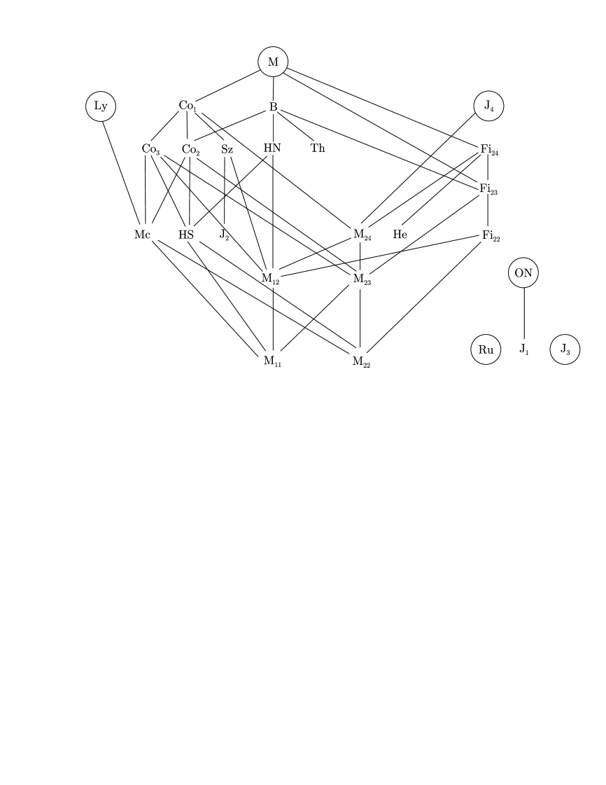
Figure 1: Genetic relation between sporadic finite simple groups [4].

4 Some applications of finite simple groups in physics

1. Elementary applications. Bose/Fermi statistics; crystal groups. Consider the Hamiltonian $H$ for a system of $N$ electrons bound in a $Z$-protons nucleus

$$H=\sum(p^{2}_{i}-Ze^{2}/r_{i})+\sum_{i\neq j}e^{2}/|{\bf r}_{i}-{\bf r}_{j}|+\text{spin forces}+\text{relativistic corrections}+\cdots.$$

This Hamiltonian deals with identical electrons, so there is an obvious symmetry $i\Longleftrightarrow j$ ($i,j:1,\dots,N$). In quantum mechanics symmetries are implemented usually by unitary operators on the Hilbert space of states. So here we must have a representation of the symmetric group ${\rm S}_{N}$. As the Jordan–Hölder chain for ${\rm S}_{N}$ is $\{Z_{2},{\rm Alt}_{N}\}$, the group has precisely two 1-dim irreps, the identical ${\rm Id}=D_{0}$ and the so-called alternant $D_{0}^{-}$. The fundamental spin-statistics theorem (Pauli, 1940) says that

“The symmetric group of a system of $N$ identical particles is represented through the 1-dim irreps; indeed, integer spin systems, called Bosons, are in the identical $D_{0}$, whereas half-integer spin particles, called Fermions, chose the alternant $D_{0}^{-}$ representations”.

In the second alternative $D_{0}^{-}$, we have the exclusion principle as a consequence (Pauli, 1925), because electrons carry spin $1/2$:

“There can be no more than one electron per orbital; or: two electrons cannot have the same (four) quantum numbers”.

The importance of this is hard to overemphasize: the whole of chemistry, up to ourselves, depends on the exclusion principle, which classifies electrons in orbitals, explains the chemical valence, etc. It is amusing to speculate as on a world, different from ours, in which the isometry group of space will not be doubly connected: in our case the rotation group ${\rm SO}(3)$ is not simply connected, so its projective representations include those of the universal covering group, ${\rm SU}(2)$: for half integer spin we have faithful irreps of ${\rm SU}(2)$, as in the case of electrons. The exclusion principle depends essentially on this:

“The ultimate reason for the existence of the valence, chemistry and ourselves is that the isometry group of our space is not simply connected, allowing genuine projective $($half-integer spin$)$ representations of the rotation group ${\rm SO}(3)$, which, in turn, carry the alternant irrep of the symmetric group, giving rise to the exclusion principle”.

As another application of finite groups in physics we just mention passim the classification of crystallographic groups, carried out first by Bravais (ca. 1850), which uses the groups of elementary polytopes (cubic lattices etc.). For instance, the icosahedron $Y_{3}$ has as rotation isometry the group ${\rm Alt}_{5}$; acting on the 12 vertices, the diagram explaining the situation is

$$\begin{array}[]{@{}ccccc}Z_{5}&\rightarrow&{\rm Alt}_{5}&\rightarrow&Y_{3}(V)\\ \downarrow&&\downarrow&&\downarrow\\ {\rm SO}(2)&\rightarrow&{\rm SO}(3)&\rightarrow&S^{2}\end{array}$$

Some viruses crystallize in icosahedra.

2. Sphere packings, codes, etc. Finite groups appear often in the sphere packing and kissing and covering problems; [19] is the standard source. Related is the question of optimal transmission of coded messages; the Leech lattice was discovered in this context (1967). Sporadic groups in the first two levels are very much related to these problems (e.g. the binary Golay code, whose automorphism group is again ${\rm M}_{24}$, see also [20]), but we do not elaborate on this engineering problem.

3. The Monster groups: string theory, vertex operators and black holes. For a recent review of finite groups in particle physics, see [30]. For relations between sporadic groups and String theory see [31].

The relation between the Monster and string theory (and/or superstrings) will be briefly referred to here [28, 26, 27]. An expansion like (4) was interpreted, from the Monster ($\mathbb{M}$) point of view, as a graded algebra, with a (reducible) representation of $\mathbb{M}$ in each level. Analogous things happen with Lie algebras $L$, there is an extension (affine Kac–Moody algebras, 1964) $L^{\widehat{\,}}$, whose natural $\infty$-dim representation supports a graded representation of $L$ [33]. Even for some Lie groups (like $E_{8}$) a “moonshine phenomenon” appears [26, 29], as another modular function plays a rôle. These generalized Lie algebras are very apt to describe String Theory as a bidimensional conformal field theory embedded in (25,1) dimensions, as in the primitive bosonic string theory; the numbers $25-1=24=8\cdot 3$ always playing a role, see also [31].

$\mathbb{M}$ and the BTZ 3-d black hole. In 1993 Bañados, Teitelboim and Zanelli (BTZ; from Chile) found a special black hole appearing in 3-dim General Relativity with a negative cosmological constant (as in 3-dim the Ricci tensor equals the Riemann tensor, pure 3-dim gravitation as such is uninteresting). In 2007 E. Witten [34] suggested a possible relation between the Monster group $\mathbb{M}$ and the BTZ black hole: the entropy of that hole might be related to the order of some variable in the Monster; indeed, for the first faithful irrep, we have $d_{2}=196883$, which is related to number of states as

$$\log(d_{1}+d_{2})=\log(196884)=12.190,$$

tantalizingly close to $4\pi=12.566$.

4. $\boldsymbol{{\rm M}_{24}}$ and the K3 surface. Some recent work has been triggered by [25], who discovered that the elliptic genus of the K3 surface has a natural decomposition in terms of the dimensions of irreducible representations of the largest Mathieu group ${\rm M}_{24}$; about the K3 surface: this four-dim real manifold is unique up to homeomophisms as carrying a ${\rm SU}(2)$ holonomy group, thus being a Calabi–Yau 2-fold ${\rm CY}_{2}$. Now ${\rm CY}_{3}$ are much used in compactification in string theories to pass from ten dimensions to our realistic four, and it turns out that K3 plays a role there also, see [35].

5. Overview. We come to the end of our mini-review of finite simple groups; they appear in the abstract domains of superstrings and black hole physics, as well as in some applied physics regimes like transmission codes. One expects that these surprising applications of an old domain of pure mathematics will be increasing in the future …

Acknowledgements

Work supported by grant A/9335/07 of the PCI-AECI and grant 2007-E24/2 of DGIID-DGA. The author thanks Professors A. Andrianov (Barcelona) and L.M. Nieto (Valladolid) for the opportunity to present the material as a Seminar in the Conference on Supersymmetric Quantum Mechanics.

References

- [1]
- [2] Bonolis L., From the rise of the group concept to the stormy onset of group theory in the new quantum mechanics. A saga of the invariant characterization of physical objects, events and theories, Rivista del Nuovo Cimento 027 (2004), 1–110.
- [3] Weyl H., Theory of groups and quantum mechanics, Dover, New York, 1928.
- [4] Conway J.H., Curtis R.T., Norton S.P., Parker R.A., Wilson R.A., Atlas of finite simple groups. Maximal subgroups and ordinary characters for simple groups, Oxford University Press, Eynsham, 1985.
- [5] Thomas A.D., Wood G.V., Group tables, Shiva Mathematics Series, Vol. 2, Shiva Publishing Ltd., Cambridge, Mass., 1980.
- [6] Ramond P., Group theory. A physicist’s survey, Cambridge University Press, Cambridge, 2010.
- [7] Hall M. Jr., The theory of groups, The Macmillan Co., New York, 1959.
- [8] Wigner E.P., Group theory and its application to the quantum mechanics of atomic spectra, Pure and Applied Physics, Vol. 5, Academic Press, New York – London, 1959.
- [9] Robinson D.J.S., A course in the theory of groups, 2nd ed., Graduate Texts in Mathematics, Vol. 80, Springer-Verlag, New York, 1996.
- [10] Bogopolski O., Introduction to group theory, European Mathematical Society (EMS), Zürich, 2008.
- [11] Coxeter H.S.M., Regular polytopes, Dover Publications, Inc., New York, 1973.
- [12] Conway J.H., Smith D.A., On quaternions and octonions: their geometry, arithmetic, and symmetry, A K Peters, Ltd., Natick, MA, 2003.
- [13] Besche H.U., Eick B., O’Brien E.A., A millennium project: constructing small groups, Internat. J. Algebra Comput. 12 (2002), 623–644.
- [14] Coxeter H.S.M., Moser W.O.J., Generators and relations for discrete groups, Springer-Verlag, New York – Heidelberg, 1972.
- [15] Carter R.W., Simple groups of Lie type, Pure and Applied Mathematics, Vol. 28, John Wiley & Sons, London – New York – Sydney, 1972.
- [16] Artin E., Geometric algebra, Interscience Publishers, Inc., New York – London, 1957.
- [17] Dieudonné J., La géométrie des groupes classiques, Springer-Verlag, Berlin – Göttingen – Heidelberg, 1955.
- [18] Boya L.J., Campoamor-Stursberg R., Composition algebras and the two faces of , Int. J. Geom. Methods Mod. Phys. 7 (2010), 367–378, arXiv:0911.3387.
- [19] Conway J.H., Sloane N.J.A., Sphere packings, lattices and groups, Grundlehren der Mathematischen Wissenschaften, Vol. 290, Springer-Verlag, New York, 1988.
- [20] Griess R.L. Jr., Twelve sporadic groups, Springer Monographs in Mathematics, Springer-Verlag, Berlin, 1998.
- [21] Biggs N.L., White A.T., Permutation groups and combinatorial structures, London Mathematical Society Lecture Note Series, Vol. 33, Cambridge University Press, Cambridge – New York, 1979.
- [22] Boya L.J., New derivation of Mathieu groups, to appear.
- [23] Greenberg P., Mathieu groups, Courant Institute of Mathematical Sciences, New York University, New York, 1973.
- [24] Coxeter H.S.M., The beauty of geometry. Twelve essays, Dover Publications, Inc., Mineola, NY, 1999.
- [25] Eguchi T., Ooguri H., Tachikawa Y., Notes on the K3 Surface and the Mathieu group , arXiv:1004.0956.
- [26] Ganon T., Monstrous moonshine: the first twenty-five years, Bull. London Math. Soc. 38 (2006), 1–33.
- [27] Ronan M., Symmetry and the Monster. One of the greatest quests of mathematics, Oxford University Press, Oxford, 2006.
- [28] Frenkel I., Lepowsky J., Meurman A., Vertex operator algebras and the Monster, Pure and Applied Mathematics, Vol. 134, Academic Press, Inc., Boston, MA, 1988.
- [29] Harada K., “Moonshine” of finite groups, EMS Series of Lectures in Mathematics, European Mathematical Society (EMS), Zürich, 2010.
- [30] Ishimori H., Kobayashi T., Ohki H., Okada H., Shimizu Y., Tanimoto M., Non-Abelian discrete symmetries in particle physics, Prog. Theor. Phys. (2010), suppl. 183, 1–163, arXiv:1003.3552.
- [31] Borcherds R.E., Sporadic groups and string theory, in First European Congress of Mathematics, Vol. I (Paris, 1992), Progr. Math., Vol. 119, Birkhäuser, Basel, 1994, 411–421.
- [32] Borcherds R.E., Book review: “Moonshine beyond the Monster. The bridge connecting algebra, modular forms and physics” by T. Gannon, Bull. Amer. Math. Soc. 45 (2008), 675–679.
- [33] Kac V.G., Infinite-dimensional Lie algebras, 3rd ed., Cambridge University Press, Cambridge, 1990.
- [34] Witten E., Three-dimensional gravity revisited, arXiv:0706.3359.
- [35] Cheng M.C.N., K3 surface, dyons, and the Mathieu group , arXiv:1005.5415.