Determining the nuclear form factor for detection of dark matter in the relativistic mean field theory

Abstract

In this work, we derive the nuclear form factor for the spin-independent collision between the WIMPs and nucleus in terms of the relativistic mean field (RMF) theory. Comparison with the traditional form factors which are commonly used in literature is given and it is found that our results are slightly above that of the 2PF model by 4% to 8%, but deviate from the Helm form factor by 15% to 25% for the whole recoil energy spectrum of 0$\sim$ 100 keV. Moreover, taking Xe and Ge as examples, we show the dependence of the form factor on the recoil energy.

1 Introduction

Discovery of dark matter undoubtedly was one of the greatest scientific events of the 20th century, then directly searching for dark matter and identifying it will be the most important task of this century. Commonly accepted point of view [1] is that the main fraction of the dark matter in our universe which resides at the hallo of the galaxy is the cold dark matter, i.e. the weakly-interacting-massive-particles (WIMPs), and the most favorable candidate of the WIMPs is the neutralino [2], even though one cannot exclude other possibilities at the present [3, 4]. What we expect is to “see” the dark matter particles in direct search experiments and find them at the LHC [5, 6, 7]. The important step is to set experiments to directly search for such mysterious particles. Since the dark matter particles only participate in weak and gravitational interactions, the scattering cross section with normal matter is very small and makes the observation very difficult. Moreover, even though the dark matter particles are very heavy, its dispersive velocity is only $200\sim 600$ km/s [8], thus the available kinetic energy $M(v/c)^{2}/2$ is of order of keV. This kinetic energy is not enough to make any inelastic nuclear reaction such as level transitions, therefore the only effects which are observable are the phenomena related to the nucleus recoil. This makes the measurement even more difficult in comparison with the neutrino experiments.

The observation rates for spin-independent scattering can be written as [9]

$$\frac{d\sigma}{d|{\bf{p}}|^{2}} = G_{F}^{2}\frac{C}{v^{2}}F^{2}(|{\bf{q}}|)=\frac{\sigma_{0}}{4m_{r}^{2}v^{2}}F^{2}(|{\bf{q}}|),$$ (1)

where $G_{F}$ is the universal Fermi coupling constant, $\sigma_{0}$ is the cross section at zero-recoil, $m_{r}$ is the reduced mass of the WIMP and nucleus, finally $F^{2}(|{\bf{q}}|)$ is the nuclear form factor. Generally speaking, the mass density distribution of the nucleus is proportional to the charge density or the nucleon number density, hence the form factor can also be accounted from the nucleon number density in the nucleus, i.e. the nuclear density. The form factor is the Fourier transformation of the nuclear density as

$$F(q) = \frac{1}{A}\int\rho(r)e^{-i{\bf{q}}\cdot{\bf{r}}}d^{3}r$$ (2)

$$= \frac{4\pi}{A}\int\frac{r}{q}\rho(r)\sin{(qr)}dr,$$

where $\rho(r)$ is the nuclear density. Here we assume that the nucleus is spherically symmetric and it is only a function of $r$.

There are several ansatz for determining the form factor by assuming typical $\rho(r)$ functions [10, 11, 12, 13]. We will give a brief review of the more commonly adopted form factors in next section.

The importance of the form factor is obvious. In fact, one of the the goals of particle-cosmology is to identify the dark matter. The strategy is to theoretically calculate $\sigma_{0}$ in terms of various models for the WIMPs, which indeed determine how WIMPs interact with quarks in nucleon. The concrete models possess several model parameters [14, 15]. Then one can compare the theoretical results with the data to extract information about the interaction and identity of the dark matter particle which is included in $\sigma_{0}$. However, in Eq. (1), $\sigma_{0}$ is convoluted with the nuclear form factor $F(q)$ which is required to obey

$$F(0)=1.$$

Unless one can more accurately determine $F(q)$, extraction of useful information from data is impossible. Thus it is crucially important to determine the form factor. Since the recoil energy spectrum may span an energy range from a few hundreds eV to a few hundreds keV and the shape of the form factor may have different response to different recoil energies, so it is extremely important to have an accurate $F(q)$ for the full energy range. Namely, an accurate determination of not only the values, but also the shape of the $F(q)$ is necessary.

In this work, we employ the relativistic mean field (RMF) theory to determine the nuclear form factors for Xe, Ge and several other nuclei which can be used as the materials for the dark matter detectors. Thus one can first choose any potential as the initial input, by iteration he eventually finds a stable form which makes all relevant equations to be self-consistent (see the text for details), the resultant form does not depend on the initial input which can be pre-assumed by our knowledge and intuition of physics. No doubt, if the initial potential is properly chosen, the iteration would converge quickly. Generally such a resultant form factor cannot be analytical, but only be presented numerically. With powerful computers, its application for extracting information of $\sigma_{0}$ from data is not affected at all.

The article is organized as follows, after this introduction, we briefly review the forms of the nuclear form factors which are commonly adopted in literature, and then we derive necessary formulae for obtaining the form factor in terms of the RMF theory. In later section, we will present our results and make a comparison with the Helm and 2PF form factors in several figures. The last section is devoted to the discussion and analysis.

2 Nuclear form factor for the spin-independent coupling

The nuclear form factor is the Fourier transformation of the nuclear density. In this paper, we numerically calculate the nuclear density by means of the RMF theory. Namely, we are going to derive the nucleon number density (nuclear density) in Eq. (2) in terms of the RMF theory.

2.1 Several types of nuclear form factors

Here let us briefly review the form factors for the spin independent WIMP-nucleus interaction which were commonly adopted in literature.

1. The simplest form factor is the exponential form [16, 17]:

$$F(E)=\exp(-E/2Q_{0}),$$ (3)

where $E=q^{2}/2M_{A}$ is the transferred energy from the WIMP to the nucleus and $Q_{0}=1.5/(MR_{0}^{2})$. The authors of Ref.[16, 17] determined the nuclear radius R₀ as:

$$R_{0}\simeq[0.91A^{1/3}+0.3]10^{-13}\mbox{cm}.$$

2. The form of the two parameter Fermi (2PF) distribution is  [13, 18]:

$$\rho(r)=\frac{\rho_{0}}{e^{(r-c)/a}+1},$$ (4)

where $\rho_{0}$ is equal to 2$\rho(r)$ at $r=c$ and the surface thickness $t=4a\ln 3$. The parameters $c$ and $a$ for different nuclei have been determined by fitting the elastic electron scattering experiments and muonic atom spectroscopy [19]. The Fourier transform of the 2PF density Eq. (4) cannot be given as an analytical expression, but can only be presented numerically. In literature [18] it is named as the 2PF form factor.

3. The ‘folding’ charge distribution was given by Helm [10] as:

$$\rho(r)=\int\rho_{0}(r^{\prime})\rho_{1}(r-r^{\prime})d^{3}r^{\prime},$$ (5)

with certain normalization conditions. The nuclear charge density

$$\rho(r)=\rho_{0}=3Ze/4\pi R^{3},\;\;\;r\leq R$$

is an approximately uniform distribution inside a cutoff radius R, and zero outside. The distribution $\rho_{1}(r)=(1/(2\pi s^{2})^{3/2})\exp(-r^{2}/2s^{2})$ is introduced to take care of the soft edge of the nucleus where $s$ is the surface thickness. Convoluting $\rho(r)$ and $\rho_{1}(r)$, one deduces the Helm form factor [20]:

$$F(q) = \frac{3j_{1}(qR)}{qR}e^{-(qs)^{2}/2}$$ (6)

$$= 3\frac{\sin(qR)-{qR}\cos(qR)}{(qR)^{3}}e^{-(qs)^{2}/2},$$

with $j_{1}$ being the first-order spherical Bessel function. The Helm form factor is the form factor which is most commonly used in directly searching for dark matter [18, 21, 22]. Lewin et al. [13] proposed a set of parameters which are fixed by fitting the muonic atom spectroscopy [19] as:

$$R^{2} = c^{2}+\frac{7}{3}\pi^{2}a^{2}-5s^{2}$$ (7)

$$c \simeq 1.23A^{1/3}-0.6\quad\mbox{fm}$$ (8)

$$s \simeq 0.9\quad\mbox{fm},\quad a\simeq 0.52\quad\mbox{fm}.$$ (9)

4. Sick [11] proposed to use a sum of the Gaussians (SOG) to express the nuclear charge density:

$$\rho(r)=\frac{Ze}{2\pi^{3/2}\gamma^{3}}\sum_{i=1}^{N}\frac{Q_{i}}{1+2R_{i}^{2}/\gamma^{2}}\{e^{-(r-R_{i})^{2}/\gamma^{2}}+e^{-(r+R_{i})^{2}/\gamma^{2}}\},$$ (10)

where $\gamma$ is the Gaussians width. $R_{i}$ and $Q_{i}$ are the position and charge fractions of the i$-th$ Gaussian function with $\sum_{i}Q_{i}=1$. The three parameters are determined in the elastic electron scattering experiments [23]. The analytical form of the form factor is given as  [18]:

$$F(q)=e^{-q^{2}\gamma^{2}/4}\sum_{i=1}^{N}\frac{Q_{i}}{1+2R_{i}^{2}/\gamma^{2}}[\cos(qR_{i})+\frac{2R_{i}^{2}}{\gamma^{2}}\frac{\sin(qR_{i})}{qR_{i}}].$$ (11)

5. In another model, the charge density is described as a sum of the Fourier-Bessel functions up to a certain cutoff radius R. The coefficients $a_{\nu}$ of the Bessel expansions are directly extracted from the elastic electron scattering experiments. The charge density and form factor are given [12, 18]:

$$\rho(r)=\left\{\begin{array}[]{ll}\sum_{\nu=1}^{N}a_{\nu}j_{0}\left(\nu\pi r/R\right)&r\leq R,\\ 0&r\geq R,\end{array}\right.$$ (14)

$$F(q)=\frac{\sin(qR)}{qR}\frac{\sum_{\nu=1}^{N}(-1)^{N}a_{\nu}/(\nu^{2}\pi^{2}-q^{2}R^{2})}{\sum_{\nu=1}^{N}(-1)^{\nu}a_{\nu}/(\nu^{2}\pi^{2})}.$$ (15)

2.2 Nuclear density in the RMF theory

We employ the RMF theory to calculate the nuclear density in order to get the form factor for several nuclei which may be used as the materials of the dark matter detector. The RMF theory, which was first introduced by Walecka [24], has been successfully applied in various fields of nuclear physics, especially the description of nuclear ground-state observables [25, 26, 27, 28]. We adopt the RMF theory with nonlinear $\sigma$ and $\omega$ terms, which are known to provide an excellent description of the ground states of finite nuclei including unstable nuclei [29, 30]. The Lagrangian for an ordinary nucleus in the RMF theory can be written as [29]:

$${\mathcal{L}} = \bar{\Psi}_{N}(i\gamma^{\mu}\partial_{\mu}-M_{N})\Psi_{N}+\frac{1}{2}\partial_{\mu}\sigma\partial^{\mu}\sigma-\frac{1}{2}m_{\sigma}^{2}\sigma^{2}-\frac{1}{3}g_{2}\sigma^{3}-\frac{1}{4}g_{3}\sigma^{4}-g_{\sigma}\bar{\Psi}_{N}\sigma\Psi_{N}$$ (16)

$$-\frac{1}{4}\Omega_{\mu\nu}\Omega^{\mu\nu}+\frac{1}{2}m_{\omega}^{2}\omega_{\mu}\omega^{\mu}+\frac{1}{4}c_{3}(\omega_{\mu}\omega^{\mu})^{2}-g_{\omega}\bar{\Psi}_{N}\gamma^{\mu}\Psi_{N}\omega_{\mu}$$

$$-\frac{1}{4}\vec{R}_{\mu\nu}\vec{R}^{\mu\nu}+\frac{1}{2}m_{\rho}^{2}\vec{\rho}_{\mu}\cdot\vec{\rho}^{\mu}-g_{\rho}\bar{\Psi}_{N}\gamma_{\mu}\vec{\rho}^{\mu}\cdot\vec{\tau}\Psi_{N}$$

$$-\frac{1}{4}F_{\mu\nu}F^{\mu\nu}-e\bar{\Psi}_{N}\gamma_{\mu}I_{c}A^{\mu}\Psi_{N},$$

with

$$\Omega_{\mu\nu} = \partial_{\mu}\omega_{\nu}-\partial_{\nu}\omega_{\mu},$$ (17)

$$\vec{R}_{\mu\nu} = \partial_{\mu}\vec{\rho}_{\nu}-\partial_{\nu}\vec{\rho}_{\mu},$$ (18)

$$F_{\mu\nu} = \partial_{\mu}A_{\nu}-\partial_{\nu}A_{\mu},$$ (19)

where $\Psi_{N}$ is the nucleon field with the mass $M_{N}$, $\sigma$, $\omega_{\mu}$, $\vec{\rho}_{\mu}$ are defined as meson fields with masses of $m_{\sigma},m_{\omega},m_{\rho}$. $g_{\sigma}$, $g_{\omega}$ and $g_{\rho}$ are respectively the couplings $\sigma NN$, $\omega NN$, and $\rho NN$. $g_{2}$, $g_{3}$ and $c_{3}$ are coupling constants of the self-coupling terms for the $\sigma$ and $\omega$ mesons. $A_{\mu}$ is the electromagnetic (EM) field. $\vec{\tau}$ is the nucleon isospin operator and $I_{c}=(1+\tau_{3})/2$ is the projector and $\tau_{3}$ is the third component of the isospin Pauli matrices for nucleons. In the RMF theory, $\sigma$, $\omega$, $\rho$ and the EM field $A$ are classical and treated as mean fields. In the Lagrangian, there are five independent fields: $\Psi_{N}$, $\sigma$, $\omega$, $\rho$, and the EM field $A$. Employing the Euler-Lagrange equation, one can obtain five coupled equations corresponding to the five independent fields. Directly solving the equations is impossible because they are non-linear, thus one needs to introduce suitable approximations. These coupled equations can be solved in a standard way within the RMF approach [25].

We deal with static and spherically symmetric nuclei, and the meson fields depend only on radius, then the zero components $\omega^{0}$, $\rho^{03}$ and $A^{0}$ would make the dominant contributions. The equation of motion for the nucleon field is the Dirac equation where the classical fields $\sigma$, $\omega$, $\rho$, and $A$ stand as the effective potential for $\Psi_{N}$,

$$\{i\gamma_{\mu}\partial^{\mu}-[M_{N}+g_{\sigma}\sigma(r)]-g_{\omega}\gamma_{0}\omega^{0}(r)-g_{\rho}\gamma_{0}\tau_{3}\rho^{03}(r)-e\gamma_{0}I_{c}A^{0}(r)\}\Psi_{N}({\bf r},t)=0.$$ (20)

In the RMF theory the baryon field is still quantum. One can input a trial potential into Eq. (20) and solve $\Psi_{N}$, then substitute this solution into the equations for the meson and EM fields as the source terms to solve those fields. Iterating many times, the solutions would converge. The trial potential in principle can be freely chosen, but the convergence rate depends on the form of the trial potential. One can always choose a potential according to his knowledge on the nuclear structure or a reasonable intuition.

We seek for solutions for $\Psi_{N}({\bf r},t)$ which have fixed energies. The nucleon field operator $\Psi_{N}({\bf r},t)$ can be written as a sum of positive and negative solutions $u_{\alpha}({\bf r})$ and $\nu_{\alpha}({\bf r})$ where $\alpha$ stands for the complete quantum numbers of an energy eigenstates and in the second quantization picture the wave function of a fermion can be written as

$$\Psi_{N}({\bf r},t)=\sum_{\alpha}[a_{\alpha}u_{\alpha}({\bf r})e^{-iE_{\alpha}t}+b_{\alpha}^{{\dagger}}\nu_{\alpha}({\bf r})e^{iE_{\alpha}t}].$$ (21)

$a_{\alpha}$ and $b_{\alpha}^{+}$ are annihilation and creation operators of baryon and anti-baryon. The subscript $\alpha$ runs over the full set of single-particle quantum numbers. For the normal nuclei, generally the negative solution $\nu_{\alpha}({\bf r})$ can be ignored in the $no~{}sea~{}approximation~{}\cite[cite]{[\@@bibref{}{P.Ring1990}{}{}]}$ . The probability operator of the nucleon density at ${\bf r}$ is

$$\Psi_{N}^{\dagger}({\bf r},t)\Psi_{N}({\bf r},t).$$ (22)

The nuclear ground state can be expressed as

$$|\Psi_{A}>=(\Pi_{i=1}^{A}a_{i}^{{\dagger}})|0>,$$

where $|0>$ is the vacuum, A is the number of nucleons in the nucleus and the product corresponds to creating A nucleons (protons and neutrons) which are the energy eigenstates. Sandwiching the probability operator Eq. (22) between the nuclear ground state, we obtain the nuclear density as

$$\rho_{B}({\bf r})=\sum_{\alpha}u_{\alpha}^{{\dagger}}({\bf r})u_{\alpha}({\bf r}).$$ (23)

The input parameters are $M_{N}=938$ MeV, $m_{\sigma}=511.198$ MeV, $m_{\omega}=$783 MeV, $m_{\rho}=770$ MeV, $g_{\sigma}=10.0289$, $g_{\omega}=12.6139$, $g_{\rho}=4.6322$, $g_{2}=-7.2325$, $g_{3}=0.6183$, and $c_{3}=71.3075$, called as the TM1 parameter set, which was determined by fitting some experimental data of finite nuclei in Ref. [29]. This parameter set is able to describe many ground state properties of finite nuclei all over the periodic table. We calculate the nuclear densities of several nuclei from light to heavy. In Fig. (1), we show the results of nuclear densities of ¹⁶O, ²³Na, ⁴⁰Ca, ⁷²Ge, ¹²⁷I, ¹³²Xe, ²⁰⁸Pb .

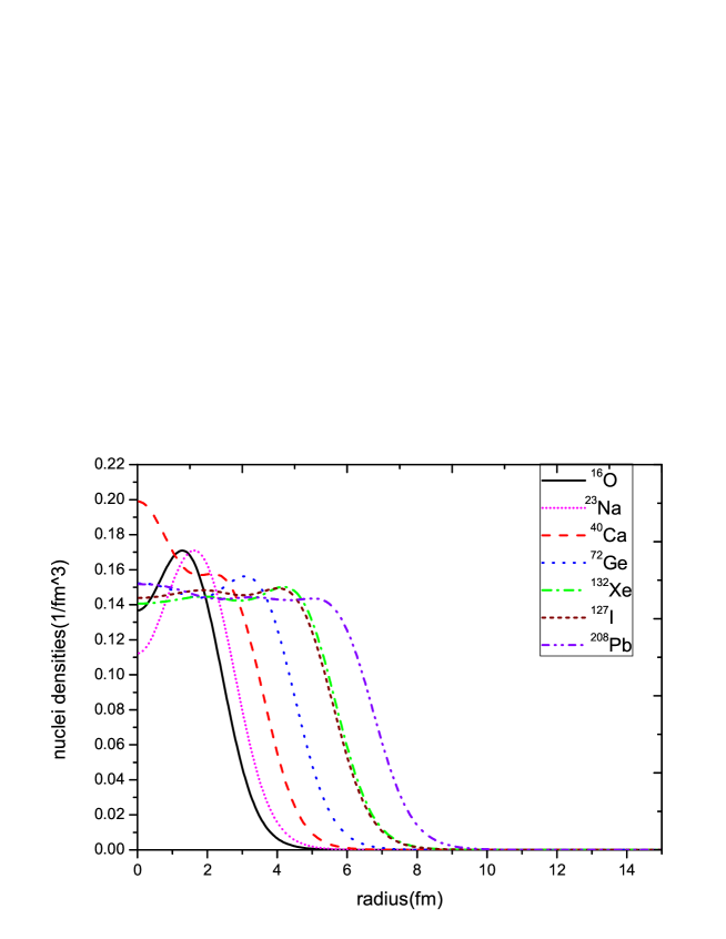
Figure 1: Nuclear densities of ¹⁶O, ²³Na, ⁴⁰Ca, ⁷²Ge, ¹²⁷I, ¹³²Xe, ²⁰⁸Pb, obtained in terms of the RMF theory.

Our next task is to perform the Fourier transformation of the RMF density numerically to gain the form factor.

The kinematics for the collisions between WIMP and nucleus: the recoil energy is

$$E={1\over 2}mv^{2}{2mM_{A}\over(m+M_{A})^{2}}(1-\cos\theta_{cm})={m_{r}^{2}v^{2}\over M_{A}}(1-\cos\theta_{cm}),$$ (24)

and the recoil three-momentum is

$$|\vec{q}|=\sqrt{2M_{A}E},$$ (25)

where $m$ and $M_{A}$ are the masses of the WIMP and nucleus respectively, $m_{r}$ is the reduced mass, $v$ is the velocity of the WIMP and $\theta_{cm}$ is the scattering angle in the center of mass frame [31]. In the lab frame, the recoil momentum is exactly the momentum transferred from the incident WIMP to the nucleus which is supposed to be at rest before impact of the WIMP.

Taking Ge as an example, in Fig. (2) we show the dependence of the RMF form factor on the recoil momentum. For a comparison we also draw the curves corresponding to the Helm and 2PF form factors. The relevant parameters of the Helm and 2PF are taken from Refs. [18, 19]. As can be seen from the Fig. (2), the results of RMF are 2% to 8% above that of 2PF form factors at most of the energy region from 2 keV (momentum q $\simeq$ 0.1 fm^-1) to 200 keV (q $\simeq$ 0.9 fm^-1), and lower by less than 1% at the range of $q\leq 0.1$ fm^-1. But at all the recoil energy regions, the RMF results are above the Helm form factor by about 15% to 25%. At 1 fm^-1, all of them attenuate to zero, or very close to zero.

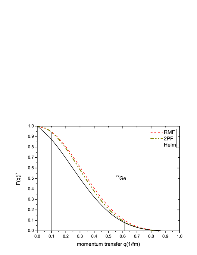
Figure 2: RMF, 2PF and Helm form factors for ⁷²Ge for the recoil energy range from 10 keV (q $\simeq$ 0.19 fm^-1 ) to 100 keV (q $\simeq$ 0.61 fm^-1 ).

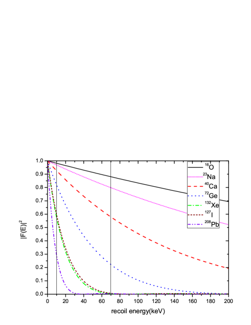
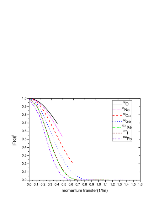
Figure 3: The RMF form factors for various nuclei corresponding to the nuclear densities shown in figure 1. The left and right pictures are the dependence of the factors as functions on respectively the recoil energy and the recoil momentum.

We plot the dependence of the RMF form factors on the recoil energy and recoil momentum (for a clearer illustration) for various nuclei in Fig. (3). It is shown that the form factor generally drops faster as the nucleus mass increases at higher recoil energies. Among the commonly adopted detector materials, F_Xe(E)(dash dot line) and F_I(E)(short dash line) have similar behaviors. They drop off more rapidly at the recoil energy range from 10 keV to 100 keV and F_Xe(E) tends to zero at 60-70 keV. It significantly influences the detection sensitivity of the Xenon detector. At the recoil energy larger than 100 keV, F_I(E) and F_Ge(E)(dot line) are too small to perform effective detections. In the case of Na and Ca, the form factors decrease more slowly in the whole energy spectrum.

3 Discussion and Conclusions

Though the RMF form factor is not analytical, its advantage is obvious. We are based on the theory which has been proved to be successful for dealing with nuclear problems, especially determining the nuclear densities for spherically or near-spherically symmetric nuclei. In the RMF theory, by resolving the Dirac equation to get nucleon wave function and with it the nuclear density can be obtained. Since this method does not depend on the initial form of the potential, even though we need to choose one for the first input, it has obvious advantage. The iteration would smear the difference between different inputs and make the final solution to converge to a should-be reliable one. Therefore we believe that the RMF form factor would be a more accurate form factor for the calculation of dark matter detection, and moreover, it also determines the energy-sensitivity curve of the material adopted for the detector.

The results can be utilized as a reference for designing dark matter detectors and make accurate extraction of information about the identity of the WIMP and its interaction with nucleon, or even with the ingredients inside nucleons (say, quarks) from data [32, 33, 34, 35, 36].

For readers’ convenience, besides the figures we presented above, we make a table where some numbers are explicitly listed. As can be seen in Table 1, at the recoil energy ranges, the form factors of the three models have ceratin differences, the RMF and 2PF form factors differ from each other by only 4%-8%, but differ by at least 15% to 25% from the Helm form factor. The Fig. (3) tells us from 10 keV to 70 keV, $F_{Xe}(E)$ obviously declines from $F_{Ge}(E)$ and $F_{I}(E)$.

Table 1: the three form factors at 10 keV, 50 keV, 100 keV , for different nucleus.

$E$	$|F(E)|^{2}$	O16	Na23	Ca40	Ge72	I127	Xe132	Pb208
10 keV	RMF	0.982	0.968	0.926	0.818	0.596	0.576	0.293
	2pF	0.981	0.965	0.920	0.802	0.605	0.579	0.305
	Helm	0.908	0.882	0.825	0.710	0.507	0.489	0.251
50 keV	RMF	0.913	0.852	0.678	0.351	0.047	0.035	0
	2pF	0.907	0.838	0.658	0.324	0.052	0.042	0
	Helm	0.777	0.706	0.545	0.278	0.040	0.031	0
100 keV	RMF	0.834	0.704	0.454	0.105	0	0	0
	2pF	0.809	0.700	0.429	0.098	0	0	0
	Helm	0.671	0.567	0.346	0.083	0	0	0

Here, We assume the target nuclei discussed in this work to be spherical or near-spherical, however realistic nuclei may be slightly deformed. Such deformations possibly affect the shape of the form factors and we are going to discuss the effects in our next work.

Acknowledgements:

This work is supported by the National Natural Science Foundation of China.

References

- [1] V. Trimble, Ann. Rev. Astron. Astrophys. 25, 425 (1987).
- [2] E. W. Kolb and M. S. Turner, ‘the Early Universe’ (Addison-Wesly, Reading, MA, 1990).
- [3] L. Bergstrom, New J. Phys. 11 105006 (2009)[arXiv:0903.4849 [hep-ph]].
- [4] J. L. Feng, arXiv:1003.0904[astro-ph.CO] (2010).
- [5] R. J. Gaitskell, Ann. Rev. Nucl. Part. Sci. 54, 315 (2004).
- [6] H. Baer, A. Belyaev, T. Krupovnickas and J. O’Farrill, JCAP 0408, 005 (2004) [arXiv:hep-ph/0405210].
- [7] H. Baer, E. K. Park and X. Tata, New J. Phys. 11, 105024 (2009) [arXiv:0903.0555 [hep-ph]].
- [8] M. Drees and C. L. Shan, JCAP 0706:011 (2007) [arXiv:astro-ph/0703651].
- [9] G. Jungman, M. Kamionkowski, K. Griest. Phys. Rept. 267,195 (1996)[arXiv:hep-ph/9506380].
- [10] R. Helm , Phys. Rev.104 1466 (1956).
- [11] I. Sick, Nucl. Phys. A 218 509-541 (1974).
- [12] Dreher et al, Nucl. Phys. A 235 219-248, (1974).
- [13] J. D. Lewin and P. F. Smith, Astropart. Phys. 6, 87 (1996).
- [14] M. W. Goodman and E. Witten,Phys. Rev. D 31, 3059 (1985).
- [15] M. Drees and M. Nojiri, Phys. Rev. D 48, 3483 (1993)[arXiv:hep-ph/9307208].
- [16] S. P. Ahlen et al., Phys. Lett. B 195, 603 (1987).
- [17] K. Freese, J. Frieman and A. Could, Phys. Rev. D 37, 3388 (1988).
- [18] G. Duda, A. Kemper and P. Gondolo, JCAP 0704, 012 (2007).
- [19] G. Fricke et al. Atomic Data and Nuclear Data Tables 60, 177-285 (1995).
- [20] J. Engel, S. Pittel and P. Vogel, Int, J. Mod. Phys. E 1 1 (1992)
- [21] J. Engel, Phys. Lett. B 264, 114 (1991)
- [22] S. Golwala, Ph.D. thesis, UC Berkeley (2000).
- [23] D. Vries et al, Atomic Data and Nuclear Data 36, 495-529 (1987)
- [24] J. D. Walecka, Ann. Phys. (N. Y.) 83, 491 (1974)
- [25] Y. K. Gambhir, P. Ring, and A.himet. Ann. Phys. (N. Y.) 198, 132 (1990).
- [26] P. Ring, Prog. Part. Nucl. Phys. 37, 193 (1996).
- [27] J. Meng, H. Toki, S. G. Zhou, S. Q. Zhang, W. H. Long, L. S. Geng, Prog. Part. Nucl. Phys. 57, 470 (2006).
- [28] X. H. Zhong, G. X. Peng, L. Li and P. Z. Ning. Phys. Rev. C 74, 034321 (2006).
- [29] Y. Sugahara and H. Toki, Nucl. Phys. A 579, 557 (1994).
- [30] H. Shen, F. Yang and H. Toki, Prog. Theor. Phys. 115, 325 (2006) [arXiv:nucl-th/0602046].
- [31] H. An, S. L. Chen, R. N. Mohapatra, S. Nussinov and Y. Zhang, Phys. Rev. D 82, 023533 (2010)[arXiv:1004.3296 [hep-ph]].
- [32] Q. P. Qiao, J. Tang, and X. Q. Li, Commun. Theor. Phys. 50: 1211-1218 (2008)[arXiv:0711.3254 [hep-ph]].
- [33] X. G. He, T. Li, X. Q. Li, J.Yandean and H. C. Tsai, Phys. Rev. D 79: 023521 (2009)[arXiv:0811.0658 [hep-ph]].
- [34] X. G. He, T. Li, X. Q. Li and H. C. Tsai, Mod. Phys. Lett. A 22: 2121-2129 (2007)[arXiv:hep-ph/0701156].
- [35] T. F. Feng, X. Q. Li, Q. W. Meng and Z. Y. Ren, Commun. Theor. Phys. 28: 347-354 (1997).
- [36] T. F. Feng, X. Q. Li, W. G. Ma, J. X. Wang and G. B. Zhao, High Energy Phys. Nucl. Phys. 30, 12 (2006)[arXiv:hep-ph/0610396].