Testing the Accretion-induced Field-decay and Spin-up Model for Recycled Pulsars

Millisecond radio pulsars have long been proposed to form from a spin-up recycling process in a binary system. In this paper we demonstrate that the accretion-induced field-decay and spin-up model for recycled pulsars can indeed produce those millisecond pulsars with relatively weak magnetic fields of $10^{8}-10^{9}$ G and short spin periods of a few milliseconds. Our results also suggest that the value of the currently observed highest spin frequency of millisecond pulsars may simply be constrained by the amount of mass available for accretion.

1 Introduction

Radio pulsars are found to be of two kinds, i.e., normal pulsars, with magnetic field $B\sim 10^{12}$ G and spin period $P\sim$ a few seconds, and millisecond pulsars (MSPs), which have low magnetic fields ($B\sim 10^{8}-10^{9}$ G) and short spin periods ($P\leq 20$ ms, e.g. Bhattacharya & van den Heuvel 1991; Lorimer 2008). These bimodal distributions in magnetic fields and spin periods are shown, e.g., in Fig. 1 in Wang et al. (2011) and also in Fig.1 of this paper, which, with data taken from ATNF pulsar catalogue, shows a large population of normal pulsars and a smaller population of MSPs. These two populations are connected with a thin bridge of pulsars in binaries. Moreover, most MSPs are in binary systems. It has long been proposed that MSPs are formed through a recycling process in which neutron stars accrete material from their low-mass companions and are spun up by the angular momentum carried by the accreted material. During this phase, the magnetic field is buried by the accreted material and decays (Alpar et al. 1982; Taam & van den Heuvel 1986; Bhattacharya & van den Heuvel 1991; Radhakrishnan & Srinivasan 1982; Bhattacharya & Srinivasan 1995; van den Heuvel 2004). These objects are therefore called recycled MSPs (Taam & van den Heuvel 1986; Bhattacharya & van den Heuvel 1991; van den Heuvel 2004).

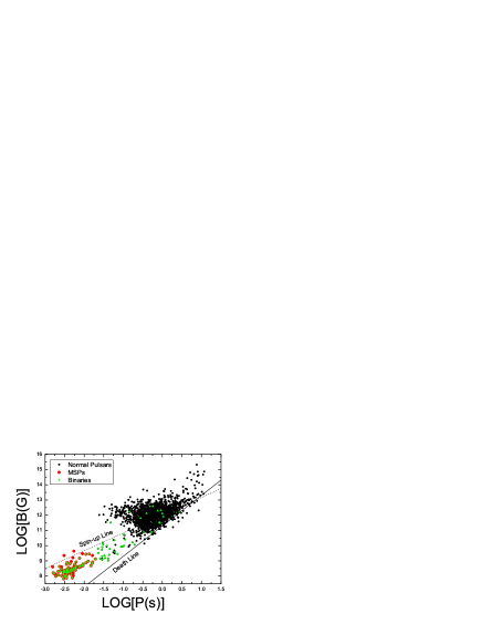
Figure 1: Magnetic fields and spin periods of observed pulsars (data taken from the ATNF pulsar catalogue). Black dots are normal pulsars. Red dots represent MSPs. Green triangles are pulsars in binaries. The ”spin-up line” represents the minimum spin-period to which a spin-up process may proceed in an Eddington-limited accretion, while the ”death-line” corresponds to a polar cap voltage below which the pulsar activity is likely to switch off (Bhattacharya & van den Heuvel 1991).

The evolutionary precursors of recycled MSPs are widely believed to be pulsars in binaries with high magnetic field ($B\sim 10^{11}-10^{13}$ G) and long spin period ($P\sim$ a few seconds, Bhattacharya & van den Heuvel 1991; Liu, van Paradijs & van den Heuvel 2007; Lorimer 2010). It is evident that $B$ and $P$ of normal pulsars and recycled pulsars are correlated with the duration of accretion phase and the total amount of accreted mass (Taam & van den Heuvel 1986; Shibazaki et al. 1989; Wijers 1997). If a neutron star accretes a small amount of mass from its companion, e.g. $\sim 0.001M_{\odot}-0.01M_{\odot}$, a recycled pulsar with mildly weak field and short spin period ($B\sim 10^{10}$ G, $P\sim 50$ ms) will be formed (e.g. Francischelli, Wijers & Brown 2002), like PSR 1913+16 and PSR J0737-3039 (Lyne et al. 2004; Kramer 2006). Strong supporting evidences for this recycling idea have been found in low mass X-ray binaries (LMXBs) containing accreting millisecond X-ray pulsars (AMXPs), e.g. SAX J 1808.4-3658 (Wijnands & van der Klis 1998), and in observing the transition link from an X-ray binary to a radio pulsar PSR J1023+0038 (Archibald et al. 2009). At the end of the accretion phase (accreted mass greater than $0.2M_{\odot}$), the neutron star magnetic field may arrive at a bottom value of about $10^{8}-10^{9}$ G and its spin period may reach a minimum of about a few milliseconds. A millisecond pulsar is formed (van den Heuvel & Bitzaraki 1995ab; Urpin, Geppert & Konenkov 1998). The accretion-induced field-decay and spin-up torque make the magnetic field and spin period (Hobbs & Manchester 2004; Manchester et al. 2005) to change from $B\sim 10^{11}-10^{13}$ G and $P\sim$ a few seconds to $B\sim 10^{8}-10^{9}$ G and $P\sim$ a few milliseconds. It is the recycling process that leads to the bimodal distribution of radio pulsars.

In this paper, we examine the accretion-induced field-decay and spin-up model of Zhang & Kojima (2006) for these recycled pulsars. We investigate the differences in model-predicted $B$ and $P$ distributions with different initial conditions. We also compare those distributions with currently observed ones. This paper is organized as the following. Section 2 gives an overview of the model. We describe the input parameters necessary in the calculations of field and spin evolutions and analyze the results in Section 3. Section 4 contains discussions and summary.

2 The model

2.1 The recycling process

A neutron star in a binary, with an initial magnetic field of about $B_{0}\sim 10^{12}$ G and an initial spin period of about $P_{0}\sim$ a few seconds, can accrete material from its companion and forms an accretion disk. When the ram pressure of accretion material equals the magnetic pressure, a magnetosphere forms. As a result, a boundary layer appears between the innermost disk and magnetosphere due to the transition for rotating velocity of plasma from Keplerian to the spin velocity of the neutron star (Inogamov & Sunyaev 1999). In this layer, the accreted matter will be channeled onto the polar patches by the field lines, where the compressed accreted matter causes the expansion of magnetic polar zone in two directions, downward and equatorward (Zhang & Kojima 2006). Therefore, the magnetic flux in the polar zone is diluted, and more matter is accreted to the polar cap and diffuses to the surface of the neutron star. Finally, the polar cap area expands and occupies the entire neutron stars surface, and the magnetic flux is buried in the equatorial area. The magnetosphere is then compressed to the neutron star surface, leading to an object with weak fields in large scale (about $\sim 10^{8}$ G) and very strong fields in small scale (about $\sim 10^{14}$ G). Meanwhile, the angular momentum carried by the accreted matter spins up the neutron star, forming a MSP with the spin period of a few milliseconds.

2.2 Magnetic field evolution

Based on the above accretion-induced field-decay and spin-up model, the accretion-induced field and spin evolution is obtained analytically: (Zhang & Kojima 2006)

$$B(t)=\frac{B_{f}}{(1-[C\,e^{-y}-1]^{2})^{\frac{7}{4}}}\,\,\,,$$ (1)

where we have $y=\frac{2\Delta M}{7M_{cr}}$, the accreted mass $\Delta M=\dot{M}t$, the crust mass $M_{cr}\sim 0.2M_{\odot}$, and $C=1+\sqrt{1-x_{0}^{2}}\sim 2$ with $x_{0}^{2}=(\frac{B_{f}}{B_{0}})^{4/7}$. $B_{0}=B(t=0)$ is the initial field strength and $B_{f}$ is the bottom magnetic field, which is defined by the neutron star magnetosphere radius matching the stellar radius, i.e., $R_{M}(B_{f})=R$. ${R_{{\rm M}}}$ is defined as $R_{M}=\phi R_{A}$ where Alfvén radius $R_{A}=3.2\times 10^{8}{\rm cm}\dot{M}^{-2/7}_{17}\mu^{4/7}_{30}m^{-1/7}$ (Elsner & Lamb 1977; Ghosh & Lamb 1977). The model dependent parameter $\phi$ is about 0.5 (Ghosh & Lamb 1979b; Shapiro & Teukolsky 1983; Frank et al. 2002). $\dot{M}_{17}$ is the accretion rate in units of $10^{17}$ g/s. $\mu_{30}$ is the magnetic moment in units of $10^{30}{\leavevmode\nobreak\ }{\rm G\leavevmode\nobreak\ cm^{3}}$. The mass $m=M/M_{\odot}$ is in the unit of solar mass. According to this model, the bottom field of neutron stars is determined by the condition that the magnetosphere radius equals the neutron stars radius (Zhang & Kojima 2006). Using the relation $R_{M}(B_{f})=R$, we can obtain the bottom field,

$$B_{f}=1.32\times 10^{8}{\rm G}(\frac{\dot{M}}{\dot{M}_{18}})^{\frac{1}{2}}m^{\frac{1}{4}}R_{6}^{-\frac{5}{4}}\phi^{-\frac{7}{4}},$$ (2)

where $\dot{M}_{18}=\dot{M}/10^{18}$ g/s and ${R_{6}}=R/10^{6}$ cm.

2.3 Spin evolution

During the accretion phase, the neutron star is spun up by the angular momentum carried by the accreted matter. The spin evolves according to the following relation given by Gosh & Lamb (1979b):

$$-\dot{P} = 5.8\times 10^{-5}[(\frac{M}{M_{\odot}})^{-\frac{3}{7}}R^{\frac{12}{7}}_{6}I_{45}^{-1}]$$

$$\times B^{\frac{2}{7}}_{12}(PL^{\frac{3}{7}}_{37})^{2}n(\omega_{s}){\leavevmode\nobreak\ \leavevmode\nobreak\ }s\leavevmode\nobreak\ yr^{-1},$$ (3)

where we define the parameters, the surface field $B_{12}=B/10^{12}$ G, the moment of inertia $I_{45}=I/10^{45}{\rm g\leavevmode\nobreak\ cm^{2}}$, the X-ray brightness ($L=GM\dot{M}/R$) $L_{37}$ in units of $10^{37}$ erg/s, respectively. The dimensionless parameter $n(\omega_{s})$ is the fastness parameter, whose expression is given by Gosh & Lamb (1979b),

$$n(\omega_{s})=1.4\times\left(\frac{1-\omega_{s}/\omega_{c}}{1-\omega_{s}}\right).$$ (4)

where $\omega_{s}$ is defined as

$$\omega_{s}\equiv\frac{\Omega_{s}}{\Omega_{k}(R_{M})}=1.35[(\frac{M}{M_{\odot}})^{-2/7}R^{15/7}_{6}]B^{6/7}_{12}P^{-1}L^{-3/7}_{37}\,\,\,,$$ (5)

with $\Omega_{s}$ being the stellar spin frequency and $\Omega_{k}$ is the Keplarian frequency. $\omega_{s}$ is the ratio parameter of the angular velocities which describes the relative importance of stellar rotation and plays a significant role in our entire understanding of accretion to the rotating magnetic neutron stars (Elsner & Lamb 1977; Ghosh & Lamb 1977; Li & Wang 1996, 1999; Shapiro & Teukolsky 1983). For a slowly rotating magnetic neutron star, $\omega_{s}\ll 1$. $\omega_{c}$ depends on several properties of the system (Gosh & Lamb 1979b) and is taken to be 0.35 in this computation.

3 $B$ and $P$ distributions of MSPs

3.1 Input parameters

According to the accretion-induced field-decay and spin-up model by Zhang & Kojima (2006), a pulsar with strong magnetic field (e.g. $B\sim 10^{12}$ G) and slow rotation ($P\sim$ a few seconds) in a binary system may be spun up to become a millisecond pulsar via accretion, and the magnetic field decays to a bottom value ($B\sim 10^{8}-10^{9}$ G) during this phase. The final state of a recycled system is characterized by the magnetic field and spin period, which are related to the initial magnetic field, initial spin period, accretion rate, accretion time, and the mass and radius of neutron stars. In computing the model-prediction of $B$ and $P$, we adopt these input parameters as the following:
(1) All precursors to recycled MSPs are assumed to be normal pulsars with magnetic field of about $B_{0}\sim 10^{12}$ G and spin period of about a few seconds. According to the data taken from ATNF catalogue, the $\log B$ and $\log P$ distributions of normal pulsars can be well described by a Gaussian function (see Wang et al. 2011). We therefore take lognormal distributions as the inputs of initial magnetic fields and spin periods. The probability density function reads,

$$p(x)=\frac{1}{\sqrt{2\pi}\sigma}\exp(-\frac{1}{2}[\frac{x-\mu}{\sigma}]^{2}),$$ (6)

where $\mu$ is the mean value of the distribution, and $\sigma$ is the standard deviation. We take $\mu=\log B({\rm G})=12$ and $\sigma=0.5$ for the $B$ distribution (see e.g. Hartman et al. 1997; Hobbs et al. 2011; Kaspi 2010; Wang et al. 2011) and $\mu=\log P({\rm s})=0$ and $\sigma=0.4$ for the $P$ distribution (see e.g. Lorimer 2010 and references therein). The range of $B$ and $P$ to consider is taken as $B_{0}=10^{10.5}-10^{14.0}$ G and $P_{0}=0.1-30$ s, respectively.
(2) The accretion rate is taken in the range from $\dot{M}=10^{16}$ g/s to $\dot{M}=10^{18}$ g/s (see e.g. Wijers 1997) and is assumed to be constant during the whole process. The duration of the accretion phase is in the range from $\Delta t=10^{7}$ yr to $\Delta t=10^{9}$ yr. Most systems may accrete $0.1-0.2M_{\odot}$ at the end of the accretion phase (see Shapiro & Teukolsky 1983). However, in some binary systems, the maximum accretion mass can be $0.6-0.8M_{\odot}$ (van den Heuvel 2011), depending on the intrinsic properties of the system. We adopt lognormal distributions (see Eq. 6) for the accretion rate and the accretion time. The mean values and standard deviations are $\mu=\log\dot{M}({\rm g/s})=17$, $\sigma=0.1$ for the accretion rate and $\mu=\log\Delta t({\rm yr})=8$, $\sigma=0.4$ for the accretion time respectively.
(3) According to recent statistics of neutron star mass (see Zhang et al. 2011), we consider a Gaussian mass distribution with the mean at $1.4M_{\odot}$ and the standard deviation equal to 0.2 $M_{\odot}$ within the range from 0.9 $M_{\odot}$ to 2.2 $M_{\odot}$.
(4) It is widely believed that the neutron star radius is about 10 km. We consider a uniform distribution of the radius from 10 km to 20 km.

3.2 Distribution of recycled MSPs

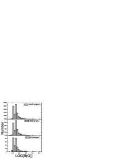
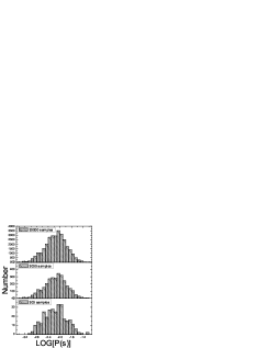
Figure 2: The computed $B$ and $P$ distributions of recycled MSPs with different numbers of random input samples. The left (right) panel is the $B$ ($P$) distribution. As discussed in the text, the computed distributions with 30000 random samples are good enough and are the ones used for comparison with observation in this work.

Figure 3: $B$ and $P$ input distributions with narrow and wide Gaussian widths (the upper panels) and their resultant final $B$ and $P$ distributions (the lower panels).

We calculated the final $B$ and $P$ according to the accretion-induced $B$ and $P$ evolution model described in section 2. In order to produce the model-predicted distribution, we generated a large number of input parameter random samples from the input parameter distributions mentioned in section 3.1. Different computation runs with 300, 3000 and 30000 samples were performed to examine how many samples are needed to have a converged result. Fig. 2 shows the $B$ and $P$ distributions of recycled MSPs obtained with 300, 3000 and 30000 random samples, respectively. We can see that, with the initial conditions considered in section 3.1, the Zhang & Kojima (2006) model indeed expects the magnetic fields of recycled MSPs are of $10^{8}-10^{9}$ G, and their spin periods are a few milliseconds. We divided these distributions into histograms with bin size of 0.1 and compared their difference with the Kolmogorov-Smirnov (K-S) test (Press et al. 1992). For the comparison of $B$ distributions between 300 and 3000 samples, the K-S statistic gives a 86.1% probability of the two being drawn from the same parent distribution. That probability for the two distributions of 3000 and 30000 samples is 100.0%. For the $P$ distributions, that probability is 64.9% for that of 300 and 3000 samples, and again reaches 100.0% for that of 3000 and 30000 samples. We therefore content ourselves with the results obtained with 30000 random samples.

Although the initial conditions, that is, input parameters, as described in section 3.1 are quite commonly adopted, we further checked the sensitivity of the model prediction results to the variation in the distribution of the input parameters. We used different input widths of the lognormal $B$ and $P$ distributions, which are 0.375 (instead of 0.5) for $B$ and 0.2 (instead of 0.4) for $P$. The ranges exploited for the $B$ and $P$ distributions are the same as in section 3.1. These input distributions and the corresponding computed final $B$ and $P$ distributions are shown Fig. 3. Based on the K-S test, the similarity between the final distributions obtained with narrow and wide inputs is 100.0%, for both $B$ and $P$ distributions. They are insensitive to mild variation of their progenitor distributions.

Finally, we compared the model-predicted $B$ and $P$ distributions with currently observed ones. The observed MSPs are usually defined as pulsars with spin period less than 20 ms. Fig. 4 shows the $B$ and $P$ distributions of observed MSPs. Because of the wide ranges of the input parameters, we have some MSPs with longer computed spin periods (see Fig. 2). The comparison with observation is conducted for spin periods shorter than 20 ms, and the computed $B$ and $P$ distributions for these recycled pulsars are plotted in Fig. 5. Again using the K-S test, we found that the degree of similarity for the $B$ distributions is $69.2\%$ and that of the $P$ distributions is $73.6\%$. We also performed a $\chi^{2}$ test to check the consistency between the model predicted distributions and observed ones. The errors in the observed distributions are assigned as $\sqrt{N_{i}}$ for each bin, where $N_{i}$ is the number of observed recycled pulsars in the $i$th bin. The $\chi^{2}$ value is $22.8$ (19 degrees of freedom) for the $B$ distribution, which corresponds to a null hypothesis probability of 24.6%, and $16.6$ (11 degrees of freedom) for the $P$ distribution, which corresponds to a 12.0% null hypothesis probability. Both the K-S test and $\chi^{2}$ test indicate that the consistency between the currently observed distributions and the Zhang & Kojima (2006) model prediction is roughly at about the so-called 1-$\sigma$ level. In other words, although not of a high degree of similarity, they are not inconsistent to each other.

Figure 4: The $B$ and $P$ distributions of observed MSPs (data taken from the ATNF pulsar catalogue).

Figure 5: The computed $B$ and $P$ distributions of recycled MSPs with spin periods shorter than 20 ms.

3.3 $B$ and $P$ evolutions of recycled MSPs

Fig. 6 displays the $B$ and $P$ evolutionary tracks during the accretion phase with initially slowly rotating and highly magnetized progenitors. In this calculation, we took the initial magnetic field as $B_{0}=5\times 10^{12}$ G and the initial spin period as $P_{0}=1$ s. Accretion rates of $10^{18}$ g/s, $10^{17}$ g/s, and $10^{16}$ g/s were considered. These tracks were followed until the accreted mass reached 1 $M_{\odot}$. The upper right panel in Fig. 6 shows that the magnetic field decays with the accumulation of the accreted material and that the bottom values of magnetic fields correlate with the accretion rates. The lower left panel shows that the pulsar rotates faster and faster when accreting more and more mass and the spin period is insensitive to the accretion rate after accreting about $0.001M_{\odot}$.

Figure 6: $B$ and $P$ evolution in the recycling process. The upper left panel shows the joint evolution of $B$ and $P$. The upper right and lower left panels are their evolution as a function of accreted mass $\Delta M$. The solid, dashed, and dotted lines are the evolutionary tracks with the accretion rate of $10^{18}$ g/s, $10^{17}$ g/s, and $10^{16}$ g/s, respectively. The initial $B$ and $P$ are taken as $B_{0}=5\times 10^{12}$ G and $P_{0}=1$ s. The lower right panel is a zoom-in view of the lower left panel in a linear scale for spin periods shorter than 5 ms.

4 Discussion and Summary

We tested the accretion-induced field-decay and spin-up model for recycled MSPs (Zhang & Kojima 2006, Wang et al. 2011). In our computation, we considered lognormal distributions of initial $B$ and $P$ in the range of $B_{0}=10^{10.5}-10^{14}$ G and $P_{0}=0.1-30$ s, a Gaussian neutron star mass distribution in the range of $M=0.9-2.2M_{\odot}$, a uniform neutron star radius distribution in $R=10-20$ km, , a lognormal distribution of the accretion rate in $\dot{M}=10^{16}-10^{18}$ g/s and of the accretion time in $\Delta t=10^{7}-10^{9}$ yr. We found that the computed $B$ and $P$ distributions of recycled MSPs are insensitive to mild variations in the width of the initial distributions. Based on the K-S test and $\chi^{2}$ test, we found that the Zhang & Kojima (2006) model prediction is consistent with observation at the 1-$\sigma$ level.

The accretion-induced field-decay model is based on the idealized idea of dilution of polar magnetic flux due to accretion. All the possible instabilities are ignored. Besides, a constant accretion rate is assumed during the whole accretion process. There are, however, some specialities for each system, such as the influence of thermal and viscous instabilities of the accretion disk and the propeller effect on the mass transfer process. The orbital angular momentum loss of the system and its causes may also have some effect on the final $B$ and $P$ state. The numerous plasma instabilities, such as the Rayleigh-Taylor instability and the Kelvin-Helmholtz instability (Ghosh & Lamb 1979a), may result in the penetration of the magnetosphere, prying the field lines aside and azimuthally wrapping the field lines by the disk matter (e.g. Romanova 2008; Kulkarni & Romanova et al. 2008), which in turn may modify the field strength evolution and then perturb the spin evolution. During the accretion, the accretion rate may change due to changes of the system and some instabilities, which can lead to the difference between the theoretical results and the actual values.

It is generally believed that there are two possible ways to form MSPs, i.e. the standard accretion-induced field-decay and spin-up model and accretion-induced collapse of white dwarfs (AIC). Due to the conservation of magnetic flux during the collapse of white dwarfs, the MSPs formed via AIC are expected to have high magnetic fields and short spin periods. Although the number of MSPs formed via AIC is no more than 20% (Zhang et al. 2011), this may also contribute to make the observed $B$ and $P$ distributions of MSPs somewhat different from that of MSPs formed via only the standard mechanism.

Some selection effects should also be noted when comparing the model prediction with observation. For example, the spin-down energy loss rate, $\dot{E}\propto\frac{B^{2}}{P^{4}}$, is related to the radio power of a pulsar. MSPs with relatively stronger magnetic fields and shorter spin periods are easier to be observed.

Owing to the ohmic dissipation, the buried field may re-emerge after accretion (e.g. Young & Chanmugam 1995; Bhattacharya 2008). Besides, If the magnetic field of recycled pulsars arrive at the bottom value at this stage and the accretion has not yet ended, the accumulation of material may spin up the recycled pulsar further. However, the magnetic field of neutron stars will not decay. The magnetic flux carried by the plasma accreted onto the neutron star surface may increase the neutron star surface field strength.

We also plot the $B$ and $P$ evolutionary scenarios during the accretion process in Fig. 6. All of these plots show that the bottom magnetic field strength is different for different accretion rates and that the minimum period is insensitive to the accretion rate at the end of the accretion phase. After accreted 1 $M_{\odot}$, the spin period reaches about 1 ms. If the there is enough mass that can be accreted (e.g. 1.2 $M_{\odot}$), the spin period can be shorter than one millisecond, forming a submillisecond pulsar. It is claimed that the maximum accreted mass is 0.8 $M_{\odot}$ under the assumption of 1 $M_{\odot}$ companion star van den Heuvel & Bitzaraki 1995a; Wijers 1997. From the recent statistics of neutron stars/LMXB (Liu, van Paradijs & van den Heuvel 2007), most neutron stars/LMXBs have the companion mass of 0.7 $M_{\odot}$. According to the accretion-induced field-decay and spin-up model, the spin period can reach the value of 1.1-1.2 ms after accreting 0.7-0.8 $M_{\odot}$. So far, the observed shortest period for MSPs is 1.4 ms (Hessels et al. 2006), and that for millisecond X-ray pulsars is 1.6 ms (e.g. Patruno 2010). Those two spin frequencies, 716 Hz and 620 Hz, are both lower than than the believed break-up spin frequency $\sim$ 1000 Hz (e.g. Lattimer & Prakash 2004). Models to explain the lack of submillisecond pulsars have been proposed, including angular momentum loss due to gravitational radiation and the magnetic spin equilibrium. A significant quadrupole moment may exist due to some oscillation modes or the so-called ’crustal mountains’ and ’magnetic deformation’, which leads to the emission of gravitational waves and the loss of angular momentum, in particularly because of its strong dependence on the spin frequency to the 5th power (e.g. Bildsten 1998; Haskell & Patruno 2011; Patruno, Haskell & D’Angelo 2011). On the other hand, however, the magnetic braking resulting from the action of stellar wind indirectly carries away the angular momentum (Rappaport, Verbunt & Joss 1983), which is more efficient than gravitational radiation by about 2 orders of magnitude in some close systems (Kalogera, Kolb & King 1998). Furthermore, the magnetic spin equilibrium set by disk/magnetosphere coupling seems successful in explaining the lack of submillisecond pulsars (D’Angelo & Spruit 2011; Kajava et al. 2011). In supplement to those efforts, the results of the accretion-induced field-decay and spin-up model as presented in this paper suggest that the achievable minimum spin period due to the recycling process may depend mainly on the amount of mass available for accretion, before the limiting shortest period set by the magnetic spin equilibrium is reached.

References

- (1) Alpar M. A., Cheng A. F. & Ruderman M. A. et al. 1982, Nature, 300, 728
- (2) Archibald A. M., Stairs I. H. & Ransom S. M. et al. 2009, Science, 324, 1411
- (3) Bhattacharya D. & van den Heuvel E. P. J. 1991, Phys. Rep., 203, 1
- (4) Bhattacharya D. & Srinivasan G. 1995, in X-ray Binaries, eds. Lewin W. H. G., van Paradijs J. and van den Heuvel E. P. J., (Cambridge University Press)
- (5) Bhattacharya D. 2008, AIPC, 1068, 137
- (6) Bildsten L. 1998, ApJ., 501, L89
- (7) D’Angelo, C. R., & Spruit, H. C. 2011, MNRAS, 416, 893
- (8) Elsner R. F., & Lamb F. K. 1977, ApJ., 215, 897
- (9) Francischelli G. J., Wijers R. A. M. J. & Brown G. E. 2002, ApJ, 565, 471
- (10) Frank J., King A. & Raine D. J. 2002, Accretion Power in Astrophysics, Cambridge, UK
- (11) Ghosh P. & Lamb F.K. 1977, ApJ., 217, 578
- (12) Ghosh P. & Lamb F.K. 1979a, ApJ., 232, 259
- (13) Ghosh P. & Lamb F.K. 1979b, ApJ., 234, 296
- (14) Hartman J.W. et al. 1997, 325, 1031
- (15) Haskell, B., & Patruno, A. 2011, ApJL, 738, L14
- (16) Hessels J. W., Ransom S. M. & Stairs I. H. et al. 2006, Science, 311, 1901
- (17) Hobbs G. & Manchester R. 2004, ATNF Pulsar Catalogue, http://www.atnf.csiro.au/research/pulsar/psrcat/psrcat_help.html
- (18) Hobbs G. et al. 2011, PASP, 28, 202
- (19) Inogamov N. A. & Sunyaev R. A., 1999, AstL., 25, 269
- (20) Kajava, J. J. E., Ibragimov, A., Annala, M., Patruno, A., & Poutanen, J. 2011, MNRAS, 417, 1454
- (21) Kaspi V. M. 2010, PNAS, 107, 7147, arXiv:1005.0876v1
- (22) Kalogera V., Kolb U. & King A. R. 1998, Apj., 504, 967
- (23) Kulkarni A. K., & Romanova M. M. 2008, MNRAS, 386, 673
- (24) Kramer M. et al. 2006, Science, 314, 97
- (25) Lattimer J. M. & Prakash M. 2004, Science, 304, 536
- (26) Li X. D., Wang Z. R., 1996, A&A, 307, L5
- (27) Li X. D. & Wang Z. R. 1999, ApJ, 513, 845
- (28) Liu Q. Z., van Paradijs J., van den Heuvel E. P. J. 2007, A&A, 469, 807
- (29) Lorimer D. R. 2008, Living Rev. Relativity, 11, 8 http://relativity.livingreviews.org/Articles/lrr-2008-8/
- (30) Lorimer D. R. 2010, arXiv:1008.1928[astro-ph]
- (31) Lyne A. G., Burgay M., Kramer M. et al. 2004, Science, 303, 1153
- (32) Manchester R. N., Hobbs G. B., Teoh A. & Hobbs M. 2005, AJ, 129, 1993
- (33) Shibazaki N., Murakami T., Shaham J. & Nomoto K. 1989, Nature, 342, 656
- (34) Shapiro S. L. & Teukolsky S. A. 1983, Black Holes, White Dwarfs and Neutron Stars. Wiley, New York
- (35) Patruno, A., Haskell, B., & D’Angelo, C. 2011, arXiv:1109.0536
- (36) Patruno, A. 2010, ApJ, 722, 909
- (37) Press et al. 1992, Numerical Recipes in Fortran 77. Cambridge University Press, London
- (38) Radhakrishnan V. & Srinivasan G. 1982, Curr. Science, 51, 1096
- (39) Romanova M. M., Kulkarni A. K. & Lovelace R. V. E. 2008, ApJ., 673, L171
- (40) Rappaport S., Verbunt F. & Joss P. C. 1983, ApJ., 275, 713
- (41) Taam R. E. & van den Heuvel E. P. J. 1986, ApJ., 305, 235
- (42) Urpin V., Geppert U. & Konenkov D. 1998, A&A, 331, 244
- (43) van den Heuvel E. P. J., 2004, Science, 303, 1143
- (44) van den Heuvel, E. P. J., 2011, Bulletin of the Astronomical Society of India, 39, 1
- (45) van den Heuvel E. P. J. & Bitzaraki O. 1995a, A&A, 297, L41
- (46) van den Heuvel E. P. J. & Bitzaraki O. 1995b, In: The Lives of the Neutron Stars, Kluwer Academic Publishers, Dordrecht
- (47) Wang J., Zhang C. M., Zhao Y. H., Kojima Y., Yin H. X., Song L. M. 2011, A&A, 526, A88
- (48) Wijnands R. & van der Klis M. 1998, Nature, 394, 344
- (49) Wijers R. A. M. J. 1997, MNRAS , 287, 607
- (50) Young E.J. & Chanmugam G. 1995, ApJ, 442, L53
- (51) Zhang C. M. & Kojima Y. 2006, MNRAS, 366, 137
- (52) Zhang C. M., Wang J., Zhao Y. H., Yin H. X., Song L. M., Menezes D. P., Wickramasinghe D. T., Ferrario L., Chardonnet P. 2011, A&A, 527, 83