Reduction of continuous symmetries of chaotic flows by the method of slices

Abstract

We study continuous symmetry reduction of dynamical systems by the method of slices (method of moving frames) and show that a ‘slice’ defined by minimizing the distance to a single generic ‘template’ intersects the group orbit of every point in the full state space. Global symmetry reduction by a single slice is, however, not natural for a chaotic / turbulent flow; it is better to cover the reduced state space by a set of slices, one for each dynamically prominent unstable pattern. Judiciously chosen, such tessellation eliminates the singular traversals of the inflection hyperplane that comes along with each slice, an artifact of using the template’s local group linearization globally. We compute the jump in the reduced state space induced by crossing the inflection hyperplane. As an illustration of the method, we reduce the $\textrm{SO}(2)$ symmetry of the complex Lorenz equations.

1 Introduction

In spatially-extended turbulent flows one observes similar patterns at different spatial positions and at different times. How ‘similar?’ If the flow is equivariant under a group of continuous symmetries, one way of answering this question is by measuring distances between different states in the symmetry-reduced state space ${\cal M}/G$, a space in which each group orbit (class of physically equivalent states) is represented by a single point. This distance depends on the choice of norm and on the symmetry-reduction method.

In 1980 Phil Morrison [1] showed how to derive Hamiltonian description of ideal fluid (plasma) dynamics from the Low Lagrangian [2] by a Lie symmetry reduction, which in this context amounts to the transformation from Lagrangian to Eulerian variables: the state space of position-labeled Lagrangian trajectories of ‘fluid parcels’ is reduced to a much smaller state space of Eulerian velocity fields. It is a difficult example of reduction; the reduction steps have to be executed judiciously, new variables cleverly chosen, and “one should do the Legendre transformations slowly and carefully when there are degeneracies [3].” Our goal here is different. Rather than to reduce a particular set of dynamical equations, we seek to formulate a computationally straightforward general method of reducing continuous symmetries, applicable to any high-dimensional chaotic/turbulent flow, such as the fluid flows bounded by pipes or planes. The symmetry-reduction literature is very extensive (see Refs. [4, 5] for a review), but it basically offers two approaches (a) invariant polynomial bases, and (b) methods which pick a representative point by slicing group orbits, generalizing the way in which Poincaré sections cut time-evolving trajectories. For high-dimensional flows the method of slices studied in Refs. [6, 4, 7, 5, 8] appears to be the only computationally feasible approach. Here the method is rederived as a distance minimization problem in the space of patterns.

The new results reported in this paper are: (a) A generic slice cuts across group orbits of all states in the state space (Section 2). (b) Every slice carries along with it the inflection hyperplane. We show how to compute the jump of the reduced state space trajectory (Section 2.2) whenever it crosses through such singularity (Section 3). (c) We propose to avoid these singularities (artifacts of the symmetry reduction by the method of slices) by tiling the state space with an atlas constructed from a set of local slices (Section 4). Pertinent facts about symmetries of dynamical systems are summarized in A. In B we show that for continuous symmetries with product structure (such as $\textrm{SO}(2)\times\textrm{SO}(2)$ symmetries of pipe and plane fluid flows), each symmetry induces its own inflection hyperplane.

In what follows we denote by ‘method of moving frames’ the post-processing of the full state space flow (Section 2.1), and by ‘method of slices’ the integration of flow confined to the reduced state space (Section 2.2). In practice, symmetry reduction is best carried out as post-processing, after the numerical trajectory is obtained by integrating the full state space flow. In particular, the symmetry-reduction induced singularities (Section 3) are more tractable numerically if given the full state space trajectory.

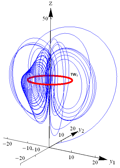
(a)         (b)

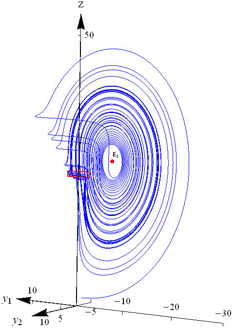
Figure 1: (a) Complex Lorenz equations (1) exhibit a strange attractor for parameter values (2), here projected on the $\{y_{1},y_{2},z\}$ axes. (thin line) A segment of generic finite time trajectory. (thick line) $\mathrm{TW}_{1}$, the only relative equilibrium. (b) The same strange attractor plotted in the symmetry-reduced state space slice (17), defined by the group tangent $\bar{t}{}^{\prime}$ whose choice is explained in (31). In the reduced state space relative equilibrium $\mathrm{TW}_{1}$ is reduced to equilibrium $\mathrm{E}_{1}$. Note, however, the semicircular jumps in the reduced flow. These are analyzed in Section 3. For a blow-up of the jump indicted by the small rectangle (red), see Fig. 4 (a).

We shall illustrate symmetry reduction by applying it to the 5-dimensional complex Lorenz equations [9]

$$\dot{x}_{1} = -\sigma x_{1}+\sigma y_{1}\,,\qquad\qquad\qquad\dot{x}_{2}\,=\,-\sigma x_{2}+\sigma y_{2}$$

$$\dot{y}_{1} = (r_{1}-z)\,x_{1}-~{}y_{1}-ey_{2}\,,\qquad\;\dot{y}_{2}\,=\,(r_{1}-z)\,x_{2}+ey_{1}-~{}y_{2}$$ (1)

$$\dot{z}~{} = -bz+x_{1}y_{1}+x_{2}y_{2}\,.$$

In all numerical calculations that follow we shall set the parameters to Ref. [5] values,

$$r_{1}=28,\;b={8}/{3},\;\sigma=10,\quad\mbox{and}\quad e={1}/{10}\,,$$ (2)

for which the flow exhibits a strange attractor, Fig. 1 (a). Our goal is to understand in detail this flow in the symmetry-reduced state space, Fig. 1 (b), in particular the singularities induced by the symmetry reduction.

A flow $\dot{x}=v(x)$ is equivariant under a coordinate transformation $g$ if the form of the equations of motion is preserved by the transformation,

$$v(x)=g^{-1}v(g\,x)\,.$$ (3)

The totality of elements $g$ forms $G$, the symmetry group of the flow. The complex Lorenz equations are a simple example of a dynamical system with a continuous (but no discrete) symmetry. They are equivariant (3) under $\textrm{SO}(2)$ rotations by

$$g({\bf\theta}) = \exp{({{\bf\theta}}\cdot T)}\,=\,\left(\begin{array}[]{ccccc}\cos{\bf\theta}&\sin{\bf\theta}&0&0&0\\ -\sin{\bf\theta}&\cos{\bf\theta}&0&0&0\\ 0&0&\cos{\bf\theta}&\sin{\bf\theta}&0\\ 0&0&-\sin{\bf\theta}&\cos{\bf\theta}&0\\ 0&0&0&0&1\end{array}\right)\,,\qquad T\,=\,\left(\begin{array}[]{ccccc}0&1&0&0&0\\ -1&0&0&0&0\\ 0&0&0&1&0\\ 0&0&-1&0&0\\ 0&0&0&0&0\end{array}\right)$$ (14)

(for group-theoretical notation, see A). The group is 1-dimensional and compact, its elements parameterized by ${\bf\theta}\mbox{ mod }2\pi$. The fixed-point subspace (37) is the $z$-axis. The velocity (1) at a point on the $z$-axis points only in the $z$-direction and so the trajectory remains on the $z$-axis for all times. The action of $\textrm{SO}(2)$ thus decomposes the state space into $m=0$ invariant subspace ($z$-axis) and $m=1$ subspace of multiplicity 2. Locally, at state space point $x$, the infinitesimal action of the group is given by the group tangent field $t(x)=Tx=(x_{2},-x_{1},y_{2},-y_{1},0)$, with the flow induced by the group action normal to the radial direction in the $(x_{1},x_{2})$ and $(y_{1},y_{2})$ planes, while the $z$-axis is left invariant.

2 Method of moving frames

Suppose you are observing turbulence in a pipe flow, or your defibrillator has a mesh of sensors measuring electrical currents that cross your heart, or you have a precomputed pattern, and are sifting through the data set of observed patterns for something like it. Here you see a pattern, and there you see a pattern that seems much like the first one. How ‘much like the first one?’ Think of the first pattern (represented by a point $\bar{x}^{\prime}$ in the state space  ${\cal M}$) as a ‘template’ [10, 6, 11] or a ‘reference state’ and use the symmetries of the flow to slide and rotate the ‘template’ until it overlays the second pattern (a point $x$ in the state space), i.e., act with elements of the symmetry group $G$ on the template $\bar{x}^{\prime}\to g({\bf\theta})\,\bar{x}^{\prime}$ until the distance between the two patterns

$$|x-g({\bf\theta})\,\bar{x}^{\prime}|=|\bar{x}-\bar{x}^{\prime}|$$ (15)

is minimized. Here $\bar{x}$ is the point on the group orbit of $x$ (the set of all points that $x$ is mapped to under the group actions),

$$x=g({\bf\theta})\,\bar{x}\,,\qquad g\in G\,,$$ (16)

closest to the template $\bar{x}^{\prime}$, the Lie group element $g=g({\bf\theta})\propto\exp{({{\bf\theta}}\cdot T)}$ is parameterized by angles ${\bf\theta}=({\bf\theta}_{1},{\bf\theta}_{2},\cdots{\bf\theta}_{N})$, and the distance is an invariant of the symmetry group, $|gx|^{2}=|x|^{2}$. We assume that $G$ is a subgroup of the group of orthogonal transformations $\textrm{O}(d)$, and measure distance $|x|^{2}=\langle{x}\vphantom{x}|\vphantom{x}{x}\rangle$ in terms of the Euclidean inner product $\langle{x}\vphantom{y}|\vphantom{x}{y}\rangle=\sum_{i}^{d}{x}_{i}y_{i}\,.$ Its Lie algebra generators $T_{a}$ (33) are $N$ linearly independent $[d\!\times\!d]$ antisymmetric matrices acting linearly on the state space vectors $x\in{\cal M}\subset\mathbb{R}^{d}$.

If the state space is a normed function space, $\langle{h}\vphantom{f}|\vphantom{h}{f}\rangle=\int dx\,h(x)f(x)\,,$ one customarily measures distance between two patterns in the $L^{2}$ norm, $|f|^{2}=\langle{f}\vphantom{f}|\vphantom{f}{f}\rangle$. In computations, spatially-extended functions are represented by discrete meshes or finite basis sets, within a (possibly large) finite-dimensional state space  ${\cal M}\subset\mathbb{R}^{d}$. An example is representation of a dissipative PDE by truncating the Fourier basis (39) to a finite number of modes.

The minimal distance is a solution of the extremum conditions

$$\frac{\partial~{}~{}}{\partial{\bf\theta}_{a}}|x-g({\bf\theta})\,\bar{x}^{\prime}|^{2}={2\,\langle{\bar{x}-\bar{x}^{\prime}}\vphantom{\bar{t}{}^{\prime}_{a}}|\vphantom{\bar{x}-\bar{x}^{\prime}}{\bar{t}{}^{\prime}_{a}}\rangle}=0\,,\qquad\bar{t}{}^{\prime}_{a}=T_{a}\bar{x}^{\prime}\,.$$

By the antisymmetry of the Lie algebra generators we have $\langle{\bar{x}^{\prime}}\vphantom{\bar{t}{}^{\prime}_{a}}|\vphantom{\bar{x}^{\prime}}{\bar{t}{}^{\prime}_{a}}\rangle=\langle{\bar{x}^{\prime}}\vphantom{T_{a}\bar{x}^{\prime}}|\vphantom{\bar{x}^{\prime}}{T_{a}\bar{x}^{\prime}}\rangle=0$, so we can replace $\bar{x}-\bar{x}^{\prime}\to\bar{x}$, and the ‘moving frame’ transformation parameters ${\bf\theta}$ which map the state $x$ to $\bar{x}$, the group orbit point closest to the template $\bar{x}^{\prime}$, satisfy

$$\langle{\bar{x}}\vphantom{\bar{t}{}^{\prime}_{a}}|\vphantom{\bar{x}}{\bar{t}{}^{\prime}_{a}}\rangle=0\,,\qquad g({\bf\theta})\,\bar{x}=x\,.$$ (17)

Thus the set of extremal group orbit points lies in a $(d\!-\!N)$-dimensional hyperplane, the set of vectors orthogonal to the template tangent space spanned by tangent vectors $\{\bar{t}{}^{\prime}_{1},\cdots,\bar{t}{}^{\prime}_{N}\}$

$$\bar{x}_{1}\bar{t}{}^{\prime}_{a,1}+\bar{x}_{2}\bar{t}{}^{\prime}_{a,2}+\cdots+\bar{x}_{d}\bar{t}{}^{\prime}_{a,d}=0\,,$$ (18)

see Fig. 2 (a). This hyperplane contains different types of extremal points. For example, the point furthest away from the template $\bar{x}^{\prime}$ also satisfies the extremal conditions. While group orbits are embedded into the high-dimensional full state space in a highly convoluted manner, this hyperplane is a linear section through them, a global extension of the tangent space of $\bar{x}^{\prime}$, which can be a good description of the ‘similarity’ to a template only in a local neighborhood of $\bar{x}^{\prime}$. Our goal is to reduce the symmetry of the flow by slicing the totality of group orbits by a small set of such neighborhoods, one for each distinct template, with each group orbit sliced only once. Group orbits close to $\bar{x}^{\prime}$ cross the hyperplane transversely; the border of the neighborhood is defined by group orbits that reach the hyperplane tangentially. In case of a local Poincaré section, determination of such border is a nontrivial task, but as we shall see in Section 3, for group orbits this border is easy to determine.

The set of the group orbit points closest to the template $\bar{x}^{\prime}$ form an open connected neighborhood of $\bar{x}^{\prime}$, a neighborhood in which each group orbit intersects the hyperplane only once. As we shall show in Section 3, this neighborhood is contained in a half-hyperplane, bounded on one side by the intersection of (18) with its inflection hyperplane. In what follows we shall refer to this connected open neighborhood of $\bar{x}^{\prime}$ as a slice $\bar{\cal M}_{\bar{x}^{\prime}}\supset{\cal M}/G$, and to (17) as the slice conditions. Slice so defined is a particular case of symmetry reduction by transverse sections of group orbits [12, 13, 14] that can be traced back to Cartan’s method of moving frames [15]. Moving frame refers to the action $g({\bf\theta})$ that brings a state space point $x$ into the slice. We denote the full state space points and velocities by $x$, $v(x)$, and the reduced state space  points and velocities by $\bar{x}$, $\bar{v}(\bar{x})$.

In the choice of the template one should avoid solutions that belong to the invariant or partially symmetric subspaces; for such choices $T_{a}\bar{x}^{\prime}=0$, and some or all $\bar{t}{}^{\prime}_{a}$ vanish identically and impose no slice conditions. The template $\bar{x}^{\prime}$ should be a generic state space point in the sense that its group orbit has the full $N$ dimensions of the group $G$. In particular, even though the simplest solutions (laminar, etc.) often capture important physical features of a flow, most equilibria and short periodic orbits have nontrivial symmetries and thus are not suited as choices of symmetry-reducing templates. It should also be emphasized that in general a template is not a spatially-localized structure. We are not using translations / rotations to superimpose a localized, ‘solitonic’ solution over a localized template. In a strongly nonlinear, turbulent flow a good template is typically a nontrivial global solution.

In summary: given the minimum Euclidean distance condition, the point $\bar{x}$ in the group orbit of $x$ closest to the template $\bar{x}^{\prime}$ lies in a slice, a hyperplane normal to the group action tangent space $\bar{t}{}^{\prime}$, for any state space point $x\in{\cal M}$. Symmetry reduction by the method of moving frames is a precise rule for how to pick a unique point $\bar{x}$ for each such symmetry equivalence class, and compute the moving frame transformation $x=g({\bf\theta})\,\bar{x}$ that relates the full state space point $x\in{\cal M}$ to its symmetry reduced representative $\bar{x}\in\bar{\cal M}$.

(a)     (b)

Figure 2: The method of moving frames. (a) Slice $\bar{\cal M}$ $(\,\,\supset{\cal M}/G)$ lies in the $(d\!-\!N)$-dimensional half-hyperplane (17) normal to $\bar{t}{}^{\prime}$, where $\bar{t}{}^{\prime}$ is the $N$-dimensional tangent to the group orbit $g\,\bar{x}^{\prime}$ (dotted line) of the template point $\bar{x}^{\prime}$, evaluated at $\bar{x}^{\prime}$. This is a highly idealized sketch: A group orbit is an $N$-dimensional manifold, and even for $\textrm{SO}(2)$ it is usually only topologically a circle, and can intersect a hyperplane any number of times. Such hyperplane intersects all full state space group orbits (indicated by dotted lines here). The full state space trajectory $x(\tau)$ and the reduced state space trajectory $\bar{x}(\tau)$ are equivalent up to a ‘moving frame’ rotation $x(\tau)=g(\tau)\,\bar{x}(\tau)$, where $g(\tau)$ is a shorthand for $g({\bf\theta}(\tau))$. (b) For $\textrm{SO}(2)$ two hyperplanes are associated with a given template $\bar{x}^{\prime}$; the slice $\bar{\cal M}$, and the hyperplane of points $x^{*}$ normal to the quadratic Casimir-weighted vector $T^{2}\bar{x}^{\prime}$, for which the curvature (23) of the distance function (15) changes sign. This defines a group-theoretic boundary of the template neighborhood: For rotation angles ${\bf\theta}$ beyond this boundary the group orbit $g({\bf\theta})\,x$ has left the neighborhood. The intersection of the two hyperplanes is the inflection hyperplane $\bar{x}^{*}\in S$, within which all group tangents $t(\bar{x}^{*})$ point into the slice and are thus normal to $\bar{t}{}^{\prime}$. For the lack of dimensions, the intersection $S$ is drawn here as a ‘line,’ the $z$ axis in this 3-dimensional sketch. $S$ is actually a $(d\!-\!2)$-dimensional hyperplane, but that is not easy to visualize.

2.1 Computing the moving frame rotation angle

The idea of reducing a flow with Lie-group structure to a system of a smaller dimension dates back to Sophus Lie. Time-evolution and symmetry group actions foliate the state space into $(N\!+\!1)$-dimensional submanifolds: Given a state (a state space point $x(0)$ at time $\tau=0$), we can trace its 1-dimensional trajectory $x(\tau)$ by integrating its equations of motion, and its $N$-dimensional group orbit by acting on it with the symmetry group $G$. Locally, a continuous time flow can be reduced by a Poincaré section; a slice does the same for local neighborhoods of group orbits.

To show how the rotation into the slice is computed, consider first the complex Lorenz equations. Substituting the $\textrm{SO}(2)$ Lie algebra generator and a finite angle $\textrm{SO}(2)$ rotation (14) acting on a 5-dimensional state space into the slice condition (17) yields $\langle{x}\vphantom{\bar{t}{}^{\prime}}|\vphantom{x}{\bar{t}{}^{\prime}}\rangle\cos{\bf\theta}-\langle{t(x)}\vphantom{\bar{t}{}^{\prime}}|\vphantom{t(x)}{\bar{t}{}^{\prime}}\rangle\sin{\bf\theta}=0\,,$ and the explicit formula for frame angle ${\bf\theta}$:

$$\tan{\bf\theta} = {\langle{x}\vphantom{\bar{t}{}^{\prime}}|\vphantom{x}{\bar{t}{}^{\prime}}\rangle}/{\langle{t(x)}\vphantom{\bar{t}{}^{\prime}}|\vphantom{t(x)}{\bar{t}{}^{\prime}}\rangle}\,.$$ (19)

The dot product of two tangent fields in (19) is a sum of inner products weighted by Casimirs (38),

$$\langle{t(x)}\vphantom{t(\bar{x}^{\prime})}|\vphantom{t(x)}{t(\bar{x}^{\prime})}\rangle=\sum_{m}C_{2}^{(m)}{x}_{i}\,\delta_{ij}^{(m)}\bar{x}^{\prime}_{j}\,.$$ (20)

For the complex Lorenz equations $x=(x_{1},x_{2},y_{1},y_{2},z)$, $\bar{x}^{\prime}=(\bar{x}_{1}^{\prime},\bar{x}_{2}^{\prime},\bar{y}_{1}^{\prime},\bar{y}_{2}^{\prime},\bar{z}^{\prime})$, and applying the moving frame condition (19) yields

$$\tan{\bf\theta}=\frac{x_{1}\bar{x}_{2}^{\prime}-x_{2}\bar{x}_{1}^{\prime}+y_{1}\bar{y}_{2}^{\prime}-y_{2}\bar{y}_{1}^{\prime}}{x_{1}\bar{x}^{\prime}_{1}+x_{2}\bar{x}^{\prime}_{2}+y_{1}\bar{y}^{\prime}_{1}+y_{2}\bar{y}^{\prime}_{2}}\,.$$ (21)

This formula is particularly simple, as in the complex Lorenz equations example the group acts only through $m=0$ and $m=1$ representations (in the Fourier mode labeling of (43)).

Consider next the general form (42) of action of an $\textrm{SO}(2)$ symmetry on arbitrary Fourier coefficients of a spatially periodic function (39). Substituting this into the slice condition (17) and using $g^{(m)}({\bf\theta})=\cos(m{\bf\theta}){\ \hbox{{\rm 1}\kern-6.00006pt\hbox{\rm 1}}}^{(m)}+\sin(m{\bf\theta})\frac{1}{m}T^{(m)}$, see (42), we find that

$$\langle{e^{-{\bf\theta}T}x}\vphantom{t(\bar{x}^{\prime})}|\vphantom{e^{-{\bf\theta}T}x}{t(\bar{x}^{\prime})}\rangle=\langle{x}\vphantom{\sum\limits_{m}\left(\cos(m{\bf\theta}){\ \hbox{{\rm 1}\kern-6.00006pt\hbox{\rm 1}}}^{(m)}+\sin(m{\bf\theta})\frac{1}{m}T^{(m)}\right)\bar{t}{}^{\prime}}|\vphantom{x}{\sum\limits_{m}\left(\cos(m{\bf\theta}){\ \hbox{{\rm 1}\kern-6.00006pt\hbox{\rm 1}}}^{(m)}+\sin(m{\bf\theta})\frac{1}{m}T^{(m)}\right)\bar{t}{}^{\prime}}\rangle$$

$${=\sum\limits_{m}\left(\langle{x}\vphantom{T^{(m)}\bar{x}^{\prime}}|\vphantom{x}{T^{(m)}\bar{x}^{\prime}}\rangle\cos(m{\bf\theta})-m\langle{x}\vphantom{{\ \hbox{{\rm 1}\kern-6.00006pt\hbox{\rm 1}}}^{(m)}\bar{x}^{\prime}}|\vphantom{x}{{\ \hbox{{\rm 1}\kern-6.00006pt\hbox{\rm 1}}}^{(m)}\bar{x}^{\prime}}\rangle\sin(m{\bf\theta})\right)}=0\,.$$ (22)

This is a polynomial equation, with coefficients determined by $\langle{x}\vphantom{T^{(m)}\bar{x}^{\prime}}|\vphantom{x}{T^{(m)}\bar{x}^{\prime}}\rangle$ and $\langle{x}\vphantom{{\ \hbox{{\rm 1}\kern-6.00006pt\hbox{\rm 1}}}^{(m)}\bar{x}^{\prime}}|\vphantom{x}{{\ \hbox{{\rm 1}\kern-6.00006pt\hbox{\rm 1}}}^{(m)}\bar{x}^{\prime}}\rangle$, as we can see by rewriting $\cos(m{\bf\theta})$, $\sin(m{\bf\theta})$ as polynomials of degree $m$ in $\sin({\bf\theta})$ and $\cos({\bf\theta})$. Each phase ${\bf\theta}$ that rotates $x$ into any of the group-orbit traversals of the slice hyperplane corresponds to a real root of this polynomial.

As a generic group orbit is a smooth $N$-dimensional manifold embedded in the $d$-dimensional state space, several values of ${\bf\theta}$ might be local extrema of the distance function (15). Our prescription is to pick the closest reduced state space point as the unique representative of the entire group orbit. i.e., determine the global minimum (infimum) of distance (15). For example, group orbits of $\textrm{SO}(2)$ are topologically circles, and the distance function has maxima, minima and inflection points as critical points: if ${\bf\theta}$ is a solution of the slice condition (19) for complex Lorenz equations, so is ${\bf\theta}+\pi$. We can pick the closest by noting that the local minima have positive curvature,

$$\frac{\partial^{2}}{\partial{\bf\theta}^{2}}|\bar{x}-\bar{x}^{\prime}|^{2}={-2\,\langle{\bar{x}}\vphantom{T^{2}\bar{x}^{\prime}}|\vphantom{\bar{x}}{T^{2}\bar{x}^{\prime}}\rangle}\,.$$ (23)

For the complex Lorenz equations, this determines which moving frame angle will be used since the distance function (15) has only a minimum and a maximum. It does not matter whether the group is compact, for example $\textrm{SO}(n)$, or noncompact, for example the Euclidean group $E_{2}$ that underlies the generation of spiral patterns [16]; in either case any group orbit has one or several locally closest passages to the template state, and generically only one that is the closest one. (Here we focus only on continuous symmetries - discrete symmetries that flows such as the Kuramoto-Sivashinsky and plane Couette flow exhibit will also have to be taken into account [17, 18, 19].)

However, ‘picking the closest’ point in a group orbit of a pattern very unlike the template is not necessarily a sensible thing to do; as such state evolves in time, distant points along its orbit can come closer to the template, causing discontinuous jumps in the moving frame angle. We shall show in Section 3 that this is a generic phenomenon for a single-slice symmetry reduction, and propose a cure in Section 4.

In summary, we do not have to compute all zeros of the slice condition (17) - all we care about is the zero that corresponds to the shortest distance (15). While post-processing of a full state space trajectory $x(\tau_{j})$ requires a numerical (Newton method) determination of the moving frame rotation ${\bf\theta}(\tau_{j})$ at each time step $\tau_{j}$, the computation is not as onerous as it might seem, as the knowledge of ${\bf\theta}(\tau_{j})$ and $t(\bar{x}(\tau_{j}))$ gives us a very good guess for ${\bf\theta}(\tau_{j+1})$. We can go a step further, and write the equations for the flow restricted to the reduced state space $\bar{\cal M}$.

2.2 Dynamics within a slice

Any state space trajectory can be written in a factorized form $x(\tau)=g(\tau)\,\bar{x}(\tau)$ (here $g(\tau)$ is a shorthand for $g({\bf\theta}(\tau))$, or perhaps even $g({\bf\theta}(x(\tau)))$). Differentiating both sides with respect to time and setting $\bar{v}={d\bar{x}}/{d\tau}$ we find $v(x)=\dot{g}\,\bar{x}+g\,\bar{v}(\bar{x})\,.$ By the equivariance (32)

$$v(\bar{x})=\bar{v}(\bar{x})+g^{-1}\,\dot{g}\,\bar{x}\,.$$

Noting that $g^{-1}\dot{g}=e^{-{\bf\theta}\cdot T}\,\frac{d~{}~{}}{d\,\tau}e^{{\bf\theta}\cdot T}=\dot{{\bf\theta}}\cdot T$, we obtain the equation for the velocity of the reduced flow:

$$\bar{v}(\bar{x})=v(\bar{x})-\dot{{\bf\theta}}(\bar{x})\cdot t(\bar{x})\,.$$ (24)

The velocity $v$ in the full state space is thus the sum of the ‘angular’ velocity (36) along the group orbit, $\dot{{\bf\theta}}\cdot t(\bar{x})$, and the remainder $\bar{v}$.

Eq. (24) is true for any factorization $x=g\bar{x}$, and by itself provides no information on how to calculate $\dot{{\bf\theta}}$. That is attained by demanding that the reduced trajectory stays within a slice, by imposing the slice conditions (17):

$$\langle{v(\bar{x})}\vphantom{\bar{t}{}^{\prime}_{a}}|\vphantom{v(\bar{x})}{\bar{t}{}^{\prime}_{a}}\rangle-\langle{\dot{{\bf\theta}}\cdot t(\bar{x})}\vphantom{\bar{t}{}^{\prime}_{a}}|\vphantom{\dot{{\bf\theta}}\cdot t(\bar{x})}{\bar{t}{}^{\prime}_{a}}\rangle=0\,.$$ (25)

This is a matrix equation in $\langle{t_{b}(\bar{x})}\vphantom{\bar{t}{}^{\prime}_{a}}|\vphantom{t_{b}(\bar{x})}{\bar{t}{}^{\prime}_{a}}\rangle$ that the authors of Refs. [11, 20] claim one can in principle solve for any Lie group. We consider here only the $\textrm{SO}(2)$ case, which has a single group tangent:

$$\bar{v}(\bar{x}) = v(\bar{x})-\dot{{\bf\theta}}(\bar{x})\,t(\bar{x})$$

$$\dot{{\bf\theta}}(\bar{x}) = {\langle{v(\bar{x})}\vphantom{\bar{t}{}^{\prime}}|\vphantom{v(\bar{x})}{\bar{t}{}^{\prime}}\rangle}/{\langle{t(\bar{x})}\vphantom{\bar{t}{}^{\prime}}|\vphantom{t(\bar{x})}{\bar{t}{}^{\prime}}\rangle}\,.$$ (26)

One way to think about this reduction of a flow to a slice is in terms of Lagrange multipliers (see Stone and Goldbart [21], Sect 1.5 for intuitive, geometrical interpretation of Lagrange multipliers). The first equation defines the flow confined to the slice, the ‘shape’, ‘template’ or ‘slice’ dynamics [6], (see Fig. 1 (b), Fig. 2 (a)), and integration of the second, ‘reconstruction’ equation [22, 23] enables us to track the corresponding trajectory in the full state space. For invariant subspaces $\dot{{\bf\theta}}=0$, so they are always included within the slice. No information is lost about the physical flow: if we know one point on a trajectory, we can hop at will back and forth between the reduced and the full state space trajectories, just as we can reconstruct a continuous trajectory from its Poincaré sections.

At this point it is worth noting that imposing the global and fixed slice (17) is not the only way to separate equivariant dynamics into ‘group dynamics’ and ‘shape’ dynamics [24]. In modern mechanics and even field theory (where elimination of group-directions is called ‘gauge-fixing’) it is natural to separate the flow locally into group dynamics and a transverse, ‘horizontal’ flow [25, 26], by the ‘method of connections’ [6]. From our point of view, such approaches are not useful, as they do not reduce the dynamics to a lower-dimensional reduced state space ${\cal M}/G$.

3 Inflection hyperplane

If two patterns are close, their group orbits are nearly parallel, and $\langle{t(x)}\vphantom{\bar{t}{}^{\prime}}|\vphantom{t(x)}{\bar{t}{}^{\prime}}\rangle\neq 0$. Hence a slice is transverse to all group orbits in an open neighborhood of the template $\bar{x}^{\prime}$, but not so globally. As we go away from the template point, the angles of the group orbit traversals can decrease all the way to zero, until their group tangents lie in the slice. This set of points defines a purely group-theoretic boundary of the template’s neighborhood (every point has a group orbit, the dynamics plays no role here, only the notion of distance). Furthermore, whenever the group tangent of the reduced state space trajectory points into the slice, the denominator in (26) vanishes and angular velocity $\dot{{\bf\theta}}$ is not defined. We now show that these singularities (a) also lie in a hyperplane, determined by the symmetry group alone, and (b) induce computable jumps in the reduced state space trajectory.

Two hyperplanes sketched in Fig. 2 (b) are associated with any given template $\bar{x}^{\prime}$; the slice (17), and the hyperplane of points $x^{*}$ defined by being normal to the quadratic Casimir-weighted vector $T^{2}\bar{x}^{\prime}$, such that from the template vantage point their group orbits are not transverse, but locally ‘horizontal,’

$$\langle{t(x^{*})}\vphantom{\bar{t}{}^{\prime}}|\vphantom{t(x^{*})}{\bar{t}{}^{\prime}}\rangle={-\langle{x^{*}}\vphantom{T^{2}\bar{x}^{\prime}}|\vphantom{x^{*}}{T^{2}\bar{x}^{\prime}}\rangle}=0$$ (27)

(for simplicity, in this section we specialize to the $\textrm{SO}(2)$ case).

We shall refer to the intersection of the two as the inflection hyperplane $S$, i.e., the set of all points $\bar{x}^{*}$ which are both (a) in the slice, and (b) whose group tangent $t(\bar{x}^{*})$ is also in the slice:

$$\langle{\bar{x}^{*}}\vphantom{\bar{t}{}^{\prime}}|\vphantom{\bar{x}^{*}}{\bar{t}{}^{\prime}}\rangle = 0$$

$$\langle{t(\bar{x}^{*})}\vphantom{\bar{t}{}^{\prime}}|\vphantom{t(\bar{x}^{*})}{\bar{t}{}^{\prime}}\rangle = {-\langle{\bar{x}^{*}}\vphantom{T^{2}\bar{x}^{\prime}}|\vphantom{\bar{x}^{*}}{T^{2}\bar{x}^{\prime}}\rangle}=0$$ (28)

(this is called ‘singular set’ in Ref. [5]). Looking back at (23), we see that $S$ is the locus of inflection points, a hyperplane through which the curvature of the distance function changes sign, and a local minimum turns into a local maximum. For example, for the complex Lorenz equations $\bar{x}^{*}=(x_{1}^{*},x_{2}^{*},y_{1}^{*},y_{2}^{*},z^{*})$, $\bar{x}^{\prime}=(x_{1}^{\prime},x_{2}^{\prime},y_{1}^{\prime},y_{2}^{\prime},z^{\prime})$, and the 3-dimensional inflection hyperplane $\bar{x}^{*}\in S\subset\bar{\cal M}$ is given by vanishing denominator in (21):

$$0={x_{1}^{*}x^{\prime}_{1}+x_{2}^{*}x^{\prime}_{2}+y_{1}^{*}y^{\prime}_{1}+y_{2}^{*}y^{\prime}_{2}}\,.$$

The inflection hyperplane $S$ is purely an artifact of the choice of a template, and has nothing to do with the dynamics; whenever the full state space trajectory crosses an inflection hyperplane, it pays it no heed whatsoever.

We next show that the singularity in the formula (19) causes a discontinuous jump in the moving frame angle ${\bf\theta}$. Consider a full state space trajectory $x(\tau)$ that passes through the inflection hyperplane (28) at time $\tau^{*}$, $\bar{x}^{*}=x(\tau^{*})$, which we shall set to $\tau^{*}=0$. At that instant the moving frame angle ${\bf\theta}$ is formally undefined: the numerator $\langle{\bar{x}^{*}}\vphantom{\bar{t}{}^{\prime}}|\vphantom{\bar{x}^{*}}{\bar{t}{}^{\prime}}\rangle$ in (19) vanishes ($\bar{x}^{*}$ is in the slice and satisfies the slice condition (17)), and the denominator ${\langle{t(\bar{x}^{*})}\vphantom{\bar{t}{}^{\prime}}|\vphantom{t(\bar{x}^{*})}{\bar{t}{}^{\prime}}\rangle}$ vanishes by (28). Nevertheless, the trajectory going through the singularity is well defined, as in the linear approximation the numerator and the denominator in the moving frame formula (19) are given by

$$\langle{x}\vphantom{\bar{t}{}^{\prime}}|\vphantom{x}{\bar{t}{}^{\prime}}\rangle = \langle{(\bar{x}^{*}+v(\bar{x}^{*})\,\tau)}\vphantom{\bar{t}{}^{\prime}_{a}}|\vphantom{(\bar{x}^{*}+v(\bar{x}^{*})\,\tau)}{\bar{t}{}^{\prime}_{a}}\rangle\,=\,\langle{v(\bar{x}^{*})}\vphantom{\bar{t}{}^{\prime}_{a}}|\vphantom{v(\bar{x}^{*})}{\bar{t}{}^{\prime}_{a}}\rangle\,\tau$$ (29)

$$\langle{t(x)}\vphantom{\bar{t}{}^{\prime}}|\vphantom{t(x)}{\bar{t}{}^{\prime}}\rangle = \langle{t(\bar{x}^{*}+v(\bar{x}^{*})\,\tau)}\vphantom{\bar{t}{}^{\prime}_{a}}|\vphantom{t(\bar{x}^{*}+v(\bar{x}^{*})\,\tau)}{\bar{t}{}^{\prime}_{a}}\rangle\,=\,\langle{t(v(\bar{x}^{*}))}\vphantom{\bar{t}{}^{\prime}_{a}}|\vphantom{t(v(\bar{x}^{*}))}{\bar{t}{}^{\prime}_{a}}\rangle\,\tau\,.$$ (30)

In other words, the moving frame rotates the state space point $x$ and the velocity $v(x)$ by the same angle, so either can be used to compute it. The shortest distance condition demands that we pick the solution with positive curvature (23), so $\langle{t(x)}\vphantom{\bar{t}{}^{\prime}}|\vphantom{t(x)}{\bar{t}{}^{\prime}}\rangle\geq 0$ for all $\tau$. As the trajectory traverses $\bar{x}^{*}$, the time $\tau$ changes the sign from negative to positive; hence we must switch from the solution $\bar{x}^{*}$ to another extremum for which $\langle{t(v(\bar{x}^{*}))}\vphantom{\bar{t}{}^{\prime}}|\vphantom{t(v(\bar{x}^{*}))}{\bar{t}{}^{\prime}}\rangle$ is positive. In the complex Lorenz flow example there are only two extrema $\{{\bf\theta},{\bf\theta}+\pi\}$, so the moving frame angle ${\bf\theta}$ jumps discontinuously by $\pi$.

Within the reduced state space  an inflection hyperplane crossing has a dramatic effect: the reduced state space flow $\bar{x}(\tau)$ jumps whenever it crosses the inflection hyperplane $\bar{x}^{*}$, by an amount that we now compute. Suppose that a reduced state space trajectory passes through a singularity $\bar{x}^{*}$ at time $\tau=\tau^{*}$. At that instant the numerator $\langle{v(\bar{x}^{*})}\vphantom{\bar{t}{}^{\prime}_{a}}|\vphantom{v(\bar{x}^{*})}{\bar{t}{}^{\prime}_{a}}\rangle$ is (generically) finite, but as the group tangent of the point $\bar{x}^{*}$ lies in the slice, ${\langle{t(\bar{x}^{*})}\vphantom{\bar{t}{}^{\prime}}|\vphantom{t(\bar{x}^{*})}{\bar{t}{}^{\prime}}\rangle}=0$ by (28), the denominator in (26) vanishes, and the angular velocity $\dot{{\bf\theta}}$ shoots off to infinity.

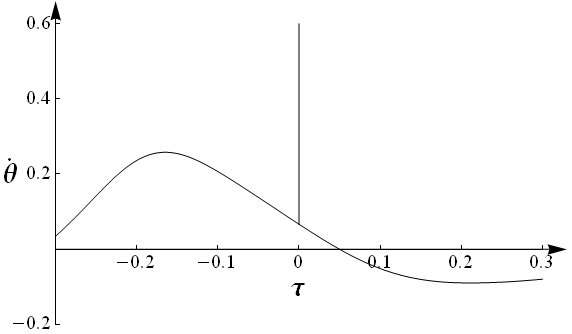
(a)    (b)

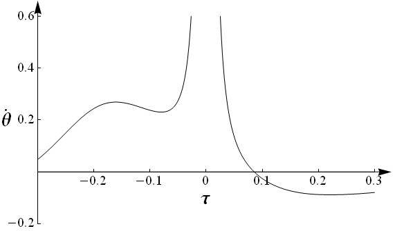
Figure 3: The angular velocity $\dot{{\bf\theta}}$ for two complex Lorenz flow reduced state space trajectories in a slice defined by the template $\bar{x}^{\prime}$ given in (31): (a) As the trajectory $\bar{x}(\tau)$ passes through the singular point $\bar{x}^{*}$ given in (31), the angular velocity diverges $\dot{{\bf\theta}}\to\infty$ as a Dirac delta function. (b) The angular velocity for a nearby trajectory going through $\bar{x}^{*}+\delta x$, $\delta x=(0.01,0,0,0,0)$ exhibits a large but finite excursion close to the singularity.

As an illustration of such jump, consider a blow-up of the small rectangle indicated in reduced state space flow Fig. 1 (b). Here the template

$$\bar{x}^{\prime} = (0.887846,-0.150461,0.4,-0.12,0)$$

$$\bar{t}{}^{\prime} = (0.150461,0.887846,0.12,0.4,0)$$ (31)

$$\bar{x}^{*} = (-0.889135,-0.0401956,1.91332,-0.150327,24.4436)$$

was reverse-engineered, by picking a point $\bar{x}^{*}=x(0)$ from a segment of the full state space ergodic trajectory $x(\tau)$ and then computing $\bar{x}^{\prime}$ such that $\bar{x}^{*}$ lies in the inflection hyperplane. As the trajectory $\bar{x}(\tau)$ passes through $\bar{x}^{*}$, the moving frame ${\bf\theta}$ jumps by $\pi$. Any trajectory nearby $x(\tau)$ in the full space (for example, the red/dashed trajectory in Fig. 4 (a)) is assigned a nearby ${\bf\theta}$ both before and after $\bar{x}(\tau)$ passes through $\bar{x}^{*}$. The closer the trajectory is to $x(\tau)$ in the full space, the shorter the time interval where its moving frame differs significantly from $x(\tau)$’s. If its symmetry-reduced trajectory does not pass through inflection hyperplane $S$, then ${\bf\theta}$ is continuous and must change by $\pi$ in a short interval of time that shrinks the closer the trajectory is to $x(\tau)$. Hence, as the trajectory $\bar{x}(\tau)$ passes through the $\bar{x}^{*}$, the angular velocity diverges $\dot{{\bf\theta}}\to\infty$ as a Dirac delta function, Fig. 3 (a), and the reduced state space trajectory goes through the inflection (28) and jumps to the $\pi$-rotated extremum of the distance function, Fig. 4 (a).

The inflection hyperplane $S$ is the intersection of two hyperplanes: (1) the slice (the shortest distance from the group-orbit to the template), and (2) the closest inflection in the distance function (28). While all group orbits of a generic trajectory cross the slice, the trajectory has vanishing probability to cross the lower-dimensional inflection hyperplane - that is why we had to ‘engineer’ the slice (31). However, an ergodic trajectory might come arbitrarily close to $S$ arbitrarily often. Such nearby reduced state space trajectories exhibit large angular velocities $\dot{{\bf\theta}}$, Fig. 3 (b), and very fast, nearly semi-circular excursions close to the singularity, Fig. 4 (a). Which segment of the group orbit they follow depends on the side from which the trajectory approached the inflection hyperplane.

(a)          (b) 

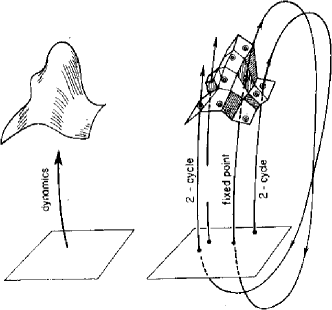
Figure 4: (color online). (a) Blow-up of a jump in Fig. 1 (b), indicated by a small rectangle. (blue/full line) A trajectory that passes through the singular point $\bar{x}^{*}$ given in (31). Note the instantaneous jump in the trajectory, caused by the divergence in velocity (Fig. 3 (a)) as the trajectory traverses the inflection hyperplane. The neighboring red/dashed trajectory going through $\bar{x}^{*}+\delta x$, $\delta x=(0,0.025,0,0,0)$, makes a rapid transit around the singularity. The green/dotted trajectory is the group orbit of $\bar{x}^{*}$ between the two ${\bf\theta}$ that rotate $v(\bar{x}^{*})$ in the slice. Note also how the red/dashed trajectory begins near the blue/full trajectory, closely follows the green/dotted trajectory after the singularity point, reaches the other side of the green/dotted arc and then resumes closely following the blue/full trajectory. (b) Smooth dynamics (left frame) tesselated by the skeleton of periodic points, together with their linearized neighborhoods, (right frame). Indicated are segments of two 1-cycles and a 2-cycle that alternates between the neighborhoods of the two 1-cycles, shadowing first one, and then the other (from ChaosBook.org).

In summary, whenever a reduced state space trajectory crosses the inflection hyperplane, it jumps instantaneously and discontinuously to the new group orbit point with the shortest distance to the template. We have shown that these jumps are harmless and theoretically under control. Nearby trajectories are numerically under control if sufficient care is taken to deal with large angular velocities. But they are an artifact of the method of slices of no dynamical significance, and an uncalled-for numerical nuisance. We now outline a strategy how to avoid them altogether by a clever choice of a set of templates.

4 Charting the reduced state space

So far, the good news is that for a generic template $\bar{x}^{\prime}$ (i.e., any $\bar{x}^{\prime}$ whose group orbit has the full $N$-dimensions of the symmetry group $G$), the slice hyperplane (17) cuts across the group orbit of every point in the full state space ${\cal M}$. But is this a useful symmetry reduction of the full state space? A distant pattern that is a bad match to a given template will have any number of locally ‘minimal’ distances, each yet another bad match. Physically it makes no sense to use a single slice (a set of all group orbit points that are closest to one given template) globally.

Work on Kuramoto-Sivashinsky and the work of Rowley and Marsden [10] suggests how to proceed: it was shown in Refs. [27, 17] that for turbulent/chaotic systems a set of Poincaré sections is needed to capture the dynamics. The choice of sections should reflect the dynamically dominant patterns seen in the solutions of nonlinear PDEs. We propose to construct a global atlas of the symmetry reduced state space ${\cal M}/G$ by deploying both slices and linear Poincaré sections across neighborhoods of the qualitatively most important patterns, taking care that the templates chosen have no symmetry. Each slice $\bar{\cal M}{}^{(j)}$, tangential to one of a finite number of templates $\bar{x}^{\prime}{}^{(j)}$, provides a local chart for a neighborhood of an important, qualitatively distinct class of solutions (2-rolls states, 3-rolls states, etc.); together they ‘Voronoi’ tessellate the curved manifold in which the reduced strange attractor is embedded by a finite set of hyperplane tiles [10, 28]. This is the symmetry-reduced generalization of the idea of state space tessellation by a set of periodic-orbits, so dear to a professional cyclist, Fig. 4 (b).

So how do we propose to implement this tessellation?

The physical task is to, for a given dynamical flow, pick a set of qualitatively distinct templates whose slices are locally tangent to the strange attractor. A ‘slice’ is a purely group-theoretic, linear construct, with no reference to dynamics; a given template $\bar{x}^{\prime}{}^{(1)}$ defines the associated slice $\bar{\cal M}$, a ($d\!-\!1$)-dimensional tangent hyperplane (for simplicity, in this section we specialize to the $\textrm{SO}(2)$ case). Within it, there is a ($d\!-\!2$)-dimensional inflection hyperplane (28). If we pick another template point $\bar{x}^{\prime}{}^{(2)}$, it comes along with its own slice and inflection hyperplane. Any neighboring pair of $(d\!-\!1)$-dimensional slices intersects in a ‘ridge’ (‘boundary,’ ‘edge’), a $(d\!-\!2)$-dimensional hyperplane, easy to compute. A global atlas so constructed should be sufficiently fine-grained that we never hit any inflection hyperplane singularities. The inflection hyperplanes should be eliminated by requiring that they lie either on the far sides of the slice-slice intersections, or elsewhere where the strange attractor does not tread. Each ‘chart’ or ‘tile,’ bounded by ridges to neighboring slices, should be sufficiently small so that the inflection hyperplane is nowhere within the part of the slice explored by the strange attractor.

Follow an ant as it traces out a symmetry-reduced trajectory $\bar{x}{}^{(1)}(\tau)$, confined to the slice $\bar{\cal M}{}^{(1)}$. The moment $\langle{\bar{x}{}^{(1)}(\tau)}\vphantom{\bar{t}{}^{\prime}{}^{(2)}}|\vphantom{\bar{x}{}^{(1)}(\tau)}{\bar{t}{}^{\prime}{}^{(2)}}\rangle$ changes sign, the ant has crossed the ridge, we symmetry-reduce with respect to the second slice, and the ant continues its merry stroll within the $\bar{\cal M}{}^{(2)}$ slice. Or, if you prefer to track the given full state space trajectory $x(\tau)$, you compute the moving-frame angle with respect to each (global) slice, and check to which tile does the given group orbit belong.

What about the fixed-point subspace ${\cal M}_{G}$ (see (37))? Because of it, the action of $G$ is globally neither free nor proper, etc.. All intersections of slices, ridges and inflection hyperplanes contain the fixed-point subspace ${\cal M}_{G}$. Should we worry? There are spurious singularities that are artifacts of a linear slice, described by the associated inflection hyperplane, and there are genuine, symmetry induced singularities, such as the embedding of an invariant subspace in the full state space (here $z$-axis). A inflection hyperplane includes the invariant subspace and cannot ‘cure’ those. Indeed, we have tried to construct an example of a two-slice chart, but for complex Lorenz equations we have not been able to find a good one. As the trajectory approaches the $z$-axis from various directions, we have not found of a way to choose two slices such that it the group orbit is tangent to one but not to the other. This is not a serious problem, as the Poincaré section and the associated return map [5] can be chosen to lie away from either inflection hyperplane.

The objective of the method of slices is to freeze [24] all equivariant coordinates; once frozen, they together with the ${\cal M}_{G}$ coordinates span the symmetry-reduced state space.

There is a rub, though - you need to know how to pick the phases of neighboring templates. This is a reflection of the flaw inherent in use of a slice hyperplane globally: a slice is derived from the Euclidean notion of distance, but for nonlinear flows the distance has to be measured curvilinearly, along unstable manifolds [29, 30]. We nevertheless have to stick with tessellation by linearized tangent spaces, as curvilinear charts appear computationally prohibitive. Perhaps a glance at Fig. 4 (b) helps visualize the problem; imagine that the trajectories drawn are group orbits, and that the tiles belong to the slices through template points on these orbits. One could slide templates along their group orbits until the pairs of straight line segments connecting neighboring template points are minimized, but that is not physical: one would like the dynamical trajectories to cross ridges as continuously as possible. So how is one to pick the phases of the templates? The phase of the first template is for free, but the moving frame transformation (16) is global, and can be applied only once. The choice of the first template thus fixes all relative phases to the succeeding templates, as was demonstrated in Ref. [17]: the universe of all other solutions is rigidly fixed through a web of heteroclinic connections between them. This insight garnered from study of a 1-dimensional Kuramoto-Sivashinsky PDE is more remarkable still when applied to the plane Couette flow [31], with 3-$d$ velocity fields and two translational symmetries. The relative phase between two templates is thus fixed by the shortest heteroclinic connection, a rigid bridge from one neighborhood to the next. Once the relative phase between the templates templates is fixed, so are their their slices, i.e., their tangent hyperplanes, and their intersection, i.e., the ridge joining them.

5 What lies ahead

Many physically important spatially-extended and fluid dynamics systems exhibit continuous symmetries. For example, excitable media [32, 33, 34, 35, 16], Kuramoto-Sivashinsky flow [36, 37, 17], plane Couette flow [38, 31, 18, 39], and pipe flow [40, 41] are invariant (equivariant) under combinations of translational (Euclidean), rotational and discrete symmetries. If a physical problem has a symmetry, one should use it - one does not want to compute the same solution over and over, all one needs is to pick one representative solution per each symmetry related equivalence class. Such procedure is called symmetry reduction. In this paper we have investigated symmetry reduction by the method of slices, a linear procedure particularly simple and practical to implement, and answered affirmatively the two main questions about the method: (1) does a slice cut the group orbit of every point in the dynamical state space? (2) can one deal with the inflection hyperplanes that the method necessarily introduces?

We have shown here that a symmetry-reduced trajectory passes through such singularities through computable jumps, a nuisance numerically, but cause to no conceptual difficulty. However, while a slice intersects each group orbit in a neighborhood of a template only once, extended globally any slice intersects every group orbit multiple times. So even though every slice cuts all group orbits, it makes no sense physically to use one slice (a set of all group orbit points that are closest to a given template) globally. We propose instead to construct a global atlas by deploying sets of slices and linear Poincaré sections as charts of neighborhoods of the most important (relative) equilibria and/or (relative) periodic orbits.

Such global atlas should be sufficiently fine-grained so that an unstable, ergodic trajectory never gets too close to any of the inflection hyperplanes. Why does this proposal have none of the elegance of, let’s say, Killing-Cartan classification of simple Lie algebras? Why is this symmetry reduction purely a numerical procedure, rather than an analytic change of equivariant coordinates to invariant ones? The theory of linear representations of compact Lie groups is a well developed subject, but role of symmetries in nonlinear settings is altogether another story. It is natural to express a dynamical system with a symmetry in the symmetry’s linear eigenfunction basis (let us say, Fourier modes), but for a nonlinear flow different modes are strongly coupled, and group orbits embedded in such coordinate bases can be highly convoluted, in ways that no single global slice hyperplane can handle intelligibly.

It should be emphasized that the atlas so constructed retains the dimensionality of the original problem. The full dynamics is faithfully retained, we are not constructing a lower-dimensional model of the dynamics. Neighborhoods of unstable equilibria and periodic orbits are dominated by their unstable and least contracting stable eigenvalues and are, for all practical purposes, low-dimensional. Traversals of the ridges are, however, higher dimensional. For example, crossing from the neighborhood of a two-rolls state into the neighborhood of a three-rolls state entails going through a pattern ‘defect,’ a rapid transient whose precise description requires many Fourier modes. Nevertheless, the recent progress on separation of ‘physical’ and ‘hyperbolically isolated’ covariant Lyapunov vectors [42, 43, 44, 45] gives us hope that the proposed atlas could provide a systematic and controllable framework for construction of lower-dimensional models of ‘turbulent’ dynamics of dissipative PDEs.

While it has been demonstrated in Ref. [5] that the method of moving frames, with a judicious choice of the template and Poincaré section, works for a system as simple as the complex Lorenz flow, one still has to show that the method can be implemented for a truly high-dimensional flow. Siminos [7] has used a modified method of moving frames to compute analytically a 128-dimensional invariant basis for reduced state space $\bar{\cal M}={\cal M}/\textrm{SO}(2)$, and shown that the unstable manifolds of relative equilibria play surprisingly important role in organizing the geometry of Kuramoto-Sivashinsky. In Ref. [17] it was found that the coexistence of four equilibria, two relative equilibria (traveling waves) and a nested fixed-point subspace structure in an effectively $8$-dimensional Kuramoto-Sivashinsky system complicates matters sufficiently that no symmetry reduction by the method of slices has been attempted so far. More importantly, a symmetry reduction of pipe flows, which due to the translational symmetry have only relative (traveling) solutions, remains an outstanding challenge [46].

Acknowledgments We sought in vain Phil Morrison’s sage counsel on how to reduce symmetries, but none was forthcoming - hence this article. We are grateful to D. Barkley, W.-J. Beyn, C. Chandre, K.A. Mitchell, B. Sandstede, R. Wilczak, and in particular E. Siminos and R.L. Davidchack for spirited exchanges. S.F. work was supported by the National Science Foundation grant DMR 0820054 and a Georgia Tech President’s Undergraduate Research Award. P.C. thanks Glen Robinson Jr. for support.

Appendix A Symmetries of dynamics

In this Appendix we review a few basic facts about dynamics and symmetries. We follow notational conventions of Chaosbook.org [30], to which the reader is referred to for a more extensive discussion of dynamics and symmetries.

If a pipe is rotated around its axis or translated, the shifted and rotated state of the fluid is a physically equivalent solution of the Navier-Stokes equations. Such rotations and translations are examples of continuous symmetries. On the level of equations of motion, one says that a flow $\dot{x}=v(x)$ is equivariant under a coordinate transformation $g$ if

$$v(x)=g^{-1}v(g\,x)\,.$$ (32)

The totality of elements $g$ forms $G$, the symmetry group of the flow. An element of a compact Lie group $G\subset\textrm{O}(d)$ that is continuously connected to the identity can be parametrized as

$$g({\bf\theta})=e^{{{\bf\theta}}\cdot T}\,,\qquad{\bf\theta}\cdot T=\sum_{a=1}^{N}{\bf\theta}_{a}T_{a}\,,$$ (33)

where ${\bf\theta}\cdot T$ is a Lie algebra element, ${\bf\theta}=({\bf\theta}_{1},{\bf\theta}_{2},\cdots{\bf\theta}_{N})$ are the parameters (‘phases,’ ‘angles,’ ‘shifts’) of the transformation, and the $T_{a}$ are a set of $N$ linearly independent $[d\!\times\!d]$ antisymmetric matrices acting linearly on the state space vectors. A spatial transformation induced by infinitesimal variations of group phases $g(\delta{\bf\theta})\simeq 1+\delta{\bf\theta}\cdot T\,.$ is

$$\delta{x}=\delta{\bf\theta}\cdot t(x)\,,$$ (34)

where the $N$ vectors

$$t_{a}(x)=T_{a}x\,,\qquad a=1,2,\cdots,N,$$ (35)

span the group tangent space at $x$. We use $t_{a}(x)$ notation (rather than $T_{a}x$) to emphasize that the group action induces a tangent field at $x$. A transformation induced by infinitesimal time-dependent variations (34) of group phases can be thought of as an ‘angular velocity,’ $\delta{\bf\theta}_{a}={\delta\tau}\,\dot{{\bf\theta}_{a}}$ is

$$\dot{x}=\dot{{\bf\theta}}\cdot t(x)\,.$$ (36)

The tangent field is of dimension $N$, as long as the point $x$ does not belong to a fixed-point subspace. Points in the fixed-point subspace ${\cal M}_{G}$ are fixed points of the full group action. They are called invariant points,

$${\cal M}_{G}=\mathrm{Fix}\left(G\right)=\{x\in{\cal M}:{g}\,x=x\mbox{ for all }g\in G\}\,,$$ (37)

or, infinitesimally, $T_{a}x=0$ for $a=1,2,\cdots,N$. If a point is an invariant point of the symmetry group, by equivariance the velocity at that point is also in ${\cal M}_{G}$, so the trajectory through that point will remain in ${\cal M}_{G}$. ${\cal M}_{G}$ is disjoint from the rest of the state space since no trajectory can ever enter or leave it.

Any representation of a compact group $G$ is fully reducible [47]. The invariant tensors constructed by contractions of $T_{a}$ are useful in identifying irreducible representations. The simplest such invariant is

$${T}\cdot T=-\sum_{m}C_{2}^{(m)}\,{\ \hbox{{\rm 1}\kern-6.00006pt\hbox{\rm 1}}}^{(m)}\,,$$ (38)

where $C_{2}^{(m)}$ is the quadratic Casimir for irreducible representation labeled $m$, and ${\ \hbox{{\rm 1}\kern-6.00006pt\hbox{\rm 1}}}^{(m)}$ is the identity on the irreducible subspace $m$, 0 elsewhere. For compact groups $C_{2}^{(m)}$ are strictly nonnegative. $C_{2}^{(m)}=0$ if $m$ is an invariant subspace.

The simplest example of a Lie group is given by the action of $\textrm{SO}(2)$ on a smooth function $u({\bf\theta}+2\pi)=u({\bf\theta})$ periodic on interval $[-\pi,\pi]$. Expand $u$ as a Fourier series

$$u({\bf\theta})=\frac{a_{0}}{2}+\sum_{m=1}^{\infty}\left(a_{m}\cos m{\bf\theta}+b_{m}\sin m{\bf\theta}\right)\,.$$ (39)

The matrix representation of the $\textrm{SO}(2)$ action $g({\bf\theta}^{\prime})u({\bf\theta})=u({\bf\theta}+{\bf\theta}^{\prime})$ on the Fourier coefficient pair $(a_{m},b_{m})$ is

$$g^{(m)}({\bf\theta}^{\prime}) = \exp{\left({{\bf\theta}^{\prime}}\cdot T^{(m)}\right)}\,=\,\left(\begin{array}[]{cc}~{}\cos m{\bf\theta}^{\prime}&\sin m{\bf\theta}^{\prime}\\ -\sin m{\bf\theta}^{\prime}&\cos m{\bf\theta}^{\prime}\end{array}\right)\,=\,\cos m{\bf\theta}^{\prime}{\ \hbox{{\rm 1}\kern-6.00006pt\hbox{\rm 1}}}^{(m)}+\sin m{\bf\theta}^{\prime}\,\frac{1}{m}T^{(m)}\,.$$ (42)

Here

$$T^{(m)}=\left(\begin{array}[]{cc}0&m\\ -m&0\end{array}\right)$$ (43)

is the Lie algebra generator and ${\ \hbox{{\rm 1}\kern-6.00006pt\hbox{\rm 1}}}^{(m)}$ is the identity on the irreducible subspace labeled $m$, 0 elsewhere. The $\textrm{SO}(2)$ group tangent $t(u)$ to state space point $u$ is

$$t(u)=\sum_{m=1}^{\infty}t^{(m)}(u)\,,\qquad t^{(m)}(u)\,=\,m\,\left(\begin{array}[]{c}~{}b_{m}\\ -a_{m}\end{array}\right)\,,$$ (44)

and the quadratic Casimir (38) for irreducible representation labeled $m$ is $C_{2}^{(m)}=m^{2}$.

Appendix B Singularities of $\textrm{SO}(2)\times\textrm{SO}(2)$

Two groups $G$ and $H$ can be combined into the product group $G\times H$, whose elements are pairs $(g,h)$, where $g$ belongs to $G$, and $h$ belongs to $H$, with the group multiplication rule $(g_{1},h_{1})(g_{2},h_{2})=(g_{1}g_{2},h_{1}h_{2})\,.$ Some important fluid-dynamical flows exhibit continuous symmetries which are the products of $\textrm{SO}(2)$ groups, each of which acts on a subset of the state space coordinates. The Kuramoto-Sivashinsky equations [36, 37], plane Couette flow [38, 31, 18], and pipe flow [40, 41] all have continuous symmetries of this form.

Let $G\times H$ be a Lie group with two sets of infinitesimal generators, $T_{1}$ and $T_{2}$, such that the $T_{1}$ acts only on the $(a)$ coordinates ($e^{{\bf\theta}_{1}T_{1}}\,(a,b)=(e^{{\bf\theta}_{1}T_{1}}a,b)$), or, infinitesimally, $T_{1}(a,b)=(T_{1}a,0)$, and $T_{2}$ acts only on the $(b)$ coordinates, $T_{2}(a,b)=(0,T_{2}b)$. Taken together, $T_{1}T_{2}(a,b)=T_{2}T_{1}(a,b)=(0,0)$ for all $(a,b)$, so $T_{1}T_{2}=0$.

For simplicity, we now specialize to the $\textrm{SO}(2)\times\textrm{SO}(2)$ case. Suppose we are rotating a trajectory $x(\tau)$ into the slice normal to the group tangents at $\bar{x}^{\prime}$. Using the restrictions the slice imposes on the angular velocity (25) yields $\langle{v(\bar{x})}\vphantom{\bar{t}{}^{\prime}_{1}}|\vphantom{v(\bar{x})}{\bar{t}{}^{\prime}_{1}}\rangle-\dot{{\bf\theta}_{1}}\langle{t_{1}(\bar{x})}\vphantom{\bar{t}{}^{\prime}_{1}}|\vphantom{t_{1}(\bar{x})}{\bar{t}{}^{\prime}_{1}}\rangle-\dot{{\bf\theta}_{2}}\langle{t_{2}(\bar{x})}\vphantom{\bar{t}{}^{\prime}_{1}}|\vphantom{t_{2}(\bar{x})}{\bar{t}{}^{\prime}_{1}}\rangle=0$. We have $\langle{t_{2}(\bar{x})}\vphantom{\bar{t}{}^{\prime}_{1}}|\vphantom{t_{2}(\bar{x})}{\bar{t}{}^{\prime}_{1}}\rangle=0$ since $T_{1}T_{2}=0$, leaving us with the equation for $\dot{{\bf\theta}_{1}}$,

$$\dot{{\bf\theta}_{1}}={\langle{v(\bar{x})}\vphantom{\bar{t}{}^{\prime}_{1}}|\vphantom{v(\bar{x})}{\bar{t}{}^{\prime}_{1}}\rangle}/{\langle{t_{1}(\bar{x})}\vphantom{\bar{t}{}^{\prime}_{1}}|\vphantom{t_{1}(\bar{x})}{\bar{t}{}^{\prime}_{1}}\rangle}\,,$$ (45)

and similarly for $\dot{{\bf\theta}_{2}}$, the same as (26) for the rotation group consisting of only the rotations generated by either $T_{1}$ or $T_{2}$. This means a point being singular depends only on whether or not it is singular in either of the slices normal to only one of the group tangents, breaking up the problem of determining if a point is singular into the same problem for each of the $\textrm{SO}(2)$ separately. In Section 3 we described what happens to the reduced state space trajectory as it passes through singularity of a single $\textrm{SO}(2)$ symmetry group. Using this result we can handle the singularities for the product of arbitrarily many $\textrm{SO}(2)$.

References

- [1] P. J. Morrison, J. M. Greene, Noncanonical Hamiltonian density formulation of hydrodynamics and ideal magnetohydrodynamics, Phys. Rev. Lett. 45 (1980) 790–794, see also Phys. Rev. Lett. 48, 569 (1982).
- [2] F. E. Low, A Lagrangian formulation of the Boltzmann-Vlasov equation for plasmas, Proc. R. Soc. London A 248 (1253) (1958) 282–287.
- [3] H. Cendra, D. D. Holm, M. J. W. Hoyle, J. E. Marsden, The Maxwell-Vlasov equations in Euler-Poincaré form, J. of Math. Phys. 39 (1998) 3138–3157.
- [4] P. Cvitanović, Chapter “Relativity for cyclists”, in Ref. [30] (2011).
- [5] E. Siminos, P. Cvitanović, Continuous symmetry reduction and return maps for high-dimensional flows, Physica D 240 (2011) 187–198.
- [6] C. W. Rowley, I. G. Kevrekidis, J. E. Marsden, K. Lust, Reduction and reconstruction for self-similar dynamical systems, Nonlinearity 16 (2003) 1257–1275.
-
[7]
E. Siminos, Recurrent spatio-temporal structures in presence of continuous
symmetries, Ph.D. thesis, School of Physics, Georgia Inst. of Technology,
Atlanta,
ChaosBook.org/projects/theses.html (2009). -
[8]
R. Wilczak, Reducing the state-space of the complex Lorenz flow, NSF REU
summer 2009 project, U. of Chicago,
ChaosBook.org/projects/Wilczak/blog.pdf (2009). - [9] J. D. Gibbon, M. J. McGuinness, The real and complex Lorenz equations in rotating fluids and lasers, Physica D 5 (1982) 108–122.
- [10] C. W. Rowley, J. E. Marsden, Reconstruction equations and the Karhunen-Loéve expansion for systems with symmetry, Physica D 142 (2000) 1–19.
- [11] S. Ahuja, I. Kevrekidis, C. Rowley, Template-based stabilization of relative equilibria in systems with continuous symmetry, J. Nonlin. Sci. 17 (2007) 109–143.
- [12] M. Fels, P. J. Olver, Moving coframes: I. A practical algorithm, Acta Appl. Math. 51 (1998) 161–213.
- [13] M. Fels, P. J. Olver, Moving coframes: II. Regularization and theoretical foundations, Acta Appl. Math. 55 (1999) 127–208.
- [14] P. J. Olver, Classical Invariant Theory, Cambridge Univ. Press, Cambridge, 1999.
- [15] E. Cartan, La méthode du repère mobile, la théorie des groupes continus, et les espaces généralisés, Vol. 5 of Exposés de Géométrie, Hermann, Paris, 1935.
- [16] D. Barkley, Euclidean symmetry and the dynamics of rotating spiral waves, Phys. Rev. Lett. 72 (1994) 164–167.
- [17] P. Cvitanović, R. L. Davidchack, E. Siminos, On the state space geometry of the Kuramoto-Sivashinsky flow in a periodic domain, SIAM J. Appl. Dyn. Syst. 9 (2010) 1–33, arXiv:0709.2944.
- [18] J. F. Gibson, J. Halcrow, P. Cvitanović, Equilibrium and traveling-wave solutions of plane Couette flow, J. Fluid Mech. 638 (2009) 243–266, arXiv:0808.3375.
- [19] P. Cvitanović, Chapter “World in a mirror”, in Ref. [30] (2011).
- [20] B. Fiedler, B. Sandstede, A. Scheel, C. Wulff, Bifurcation from relative equilibria of noncompact group actions: Skew products, meanders, and drifts, Doc. Math. 141 (1996) 479–505.
- [21] M. Stone, P. Goldbart, Mathematics for Physics: A Guided Tour for Graduate Students, Cambridge Univ. Press, Cambridge, 2009.
- [22] J. E. Marsden, Lectures on Mechanics, Cambridge Univ. Press, Cambridge, 1992.
- [23] J. E. Marsden, T. S. Ratiu, Introduction to Mechanics and Symmetry, Springer, New York, 1994.
- [24] W.-J. Beyn, V. Thümmler, Freezing solutions of equivariant evolution equations, SIAM J. Appl. Dyn. Syst. 3 (2004) 85–116.
- [25] S. Smale, Topology and mechanics, I., Inv. Math. 10 (1970) 305–331.
- [26] R. Abraham, J. E. Marsden, Foundations of Mechanics, Benjamin-Cummings, Reading, Mass., 1978.
- [27] Y. Lan, P. Cvitanović, Unstable recurrent patterns in Kuramoto-Sivashinsky dynamics, Phys. Rev. E 78 (2008) 026208, arXiv:0804.2474.
- [28] S. T. Roweis, L. K. Saul, Nonlinear dimensionality reduction by locally linear embedding, Science 290 (2000) 2323–2326.
- [29] F. Christiansen, P. Cvitanović, V. Putkaradze, Spatiotemporal chaos in terms of unstable recurrent patterns, Nonlinearity 10 (1997) 55–70, arXiv:chao-dyn/9606016.
- [30] P. Cvitanović, R. Artuso, R. Mainieri, G. Tanner, G. Vattay, Chaos: Classical and Quantum, Niels Bohr Inst., Copenhagen, 2011, ChaosBook.org.
- [31] J. F. Gibson, J. Halcrow, P. Cvitanović, Visualizing the geometry of state-space in plane Couette flow, J Fluid Mech. 611 (2008) 107–130, arXiv:0705.3957.
- [32] A. N. Zaikin, A. M. Zhabotinsky, Concentration wave propagation in 2-dimensional liquid-phase self-oscillating system, Nature 225 (1970) 535–537.
- [33] A. T. Winfree, Scroll-shaped waves of chemical activity in 3 dimensions, Science 181 (1973) 937–939.
- [34] A. T. Winfree, The Geometry of Biological Time, Springer, New York, 1980.
- [35] D. Barkley, M. Kness, L. S. Tuckerman, Spiral wave dynamics in a simple model of excitable media: Transition from simple to compound rotation, Phys. Rev. A 42 (1990) 2489–2492.
- [36] Y. Kuramoto, T. Tsuzuki, Persistent propagation of concentration waves in dissipative media far from thermal equilibrium, Progr. Theor. Phys. 55 (1976) 365–369.
- [37] G. I. Sivashinsky, Nonlinear analysis of hydrodynamical instability in laminar flames - I. Derivation of basic equations, Acta Astronaut. 4 (1977) 1177–1206.
- [38] D. Viswanath, Recurrent motions within plane Couette turbulence, J. Fluid Mech. 580 (2007) 339–358, arXiv:physics/0604062.
- [39] J. F. Gibson, P. Cvitanović, Movies of plane Couette, Tech. rep., Georgia Inst. of Technology, ChaosBook.org/tutorials (2011).
- [40] H. Wedin, R. R. Kerswell, Exact coherent structures in pipe flow, J. Fluid Mech. 508 (2004) 333–371.
- [41] R. R. Kerswell, Recent progress in understanding the transition to turbulence in a pipe, Nonlinearity 18 (2005) R17–R44.
- [42] A. Politi, F. Ginelli, S. Yanchuk, Y. Maistrenko, From synchronization to Lyapunov exponents and back, Physica D 224 (2006) 90, arXiv:nlin/0605012.
- [43] F. Ginelli, P. Poggi, A. Turchi, H. Chaté, R. Livi, A. Politi, Characterizing dynamics with covariant Lyapunov vectors, Phys. Rev. Lett. 99 (2007) 130601, arXiv:0706.0510.
- [44] H.-l. Yang, K. A. Takeuchi, F. Ginelli, H. Chaté, G. Radons, Hyperbolicity and the effective dimension of spatially-extended dissipative systems, Phys. Rev. Lett. 102 (2009) 074102, arXiv:0807.5073.
- [45] K. A. Takeuchi, F. Ginelli, H. Chaté, Lyapunov analysis captures the collective dynamics of large chaotic systems, Phys. Rev. Lett. 103 (2009) 154103, arXiv:0907.4298.
- [46] A. P. Willis, A. Avila, P. Cvitanović, B. Hof, Reduction of continuous symmetries of pipe flows by the method of slices, in preparation (2011).
- [47] B. C. Hall, Lie Groups, Lie Algebras, and Representations, Springer, New York, 2003.