Light-front zero-mode contribution to the tensor form factors for the exclusive rare $P\to V\ell^{+}\ell^{-}$ decays

Abstract

We study the light-front zero-mode contribution to the tensor form factors $T_{i}(i=1,2,3)$ for the exclusive rare $P\to V\ell^{+}\ell^{-}$ decays using a covariant fermion field theory model in $(3+1)$ dimensions. While the zero-mode contribution in principle depends on the form of the vector meson vertex $\Gamma^{\mu}=\gamma^{\mu}-(2k-P_{V})^{\mu}/D$, the three tensor form factors $T_{i}(i=1,2,3)$ are found to be free from the zero mode if the denominator $D$ contains the term proportional to the light-front energy or the longitudinal momentum fraction factor $(1/x)^{n}$ of the struck quark with the power $n>0$. Since the denominator $D$ used in the light-front quark model (LFQM) has the power $n=1/2$, the three tensor form factors $T_{i}(i=1,2,3)$ can be computed in LFQM safely without involving any complicate zero-mode contribution. The lack of zero-mode contribution benefits the phenomenology with LFQM.

The study of $B$ meson physics is important not only in extracting the most accurate values of the Cabibbo-Kobayashi-Maskawa (CKM) matrix elements [1] but also in searching for new physics effects beyond the standard model (SM). Especially, the flavor-changing neutral current (FCNC) processes of $B\to K^{(*)}\ell^{+}\ell^{-}(\ell=e,\mu,\tau)$ that proceed via loop diagrams [2] in the SM are very important for not only testing the SM but also probing new physics such as supersymmetric heavy particles in SUSY models, appearing virtually in the loop diagrams to interfere with those in the SM. While the experimental tests of exclusive decays are much easier than those of inclusive ones, the theoretical understanding of exclusive decays is complicated mainly due to the nonperturbative hadronic form factors entered in the long-distance nonperturbative contributions. Therefore, a reliable estimate of the hadronic form factors for the exclusive rare $B$ decays is very important for making correct predictions within and beyond the SM.

Perhaps, one of the most well-suited formulations for the analysis of exclusive processes involving hadrons may be provided in the framework of light-front (LF) quantization [3]. For its simplicity and the predictive power of the hadronic form factors in low-lying ground-state hadrons, especially mesons, the LF constituent quark model (LFQM) based on the LF quantization has become a very useful and popular phenomenological tool to study various electroweak properties of mesons [4, 5, 6, 7, 8, 9, 10, 11]. However, the zero-mode complication [12] in the matrix element has been noticed for the electroweak form factors involving a spin-0 and spin-1 particles [13, 14, 15]. The zero mode can be interpreted as residues of virtual pair creation processes in the $q^{+}(=q^{0}+q^{3})\to 0$ limit, i.e., the nonzero contribution from the nonvalence part in the $q^{+}=0$ frame [12]. Therefore, finding the zero-mode contribution correctly in various electroweak transitions is a very important issue in LF hadron phenomenology.

In our previous works, we have studied the zero-mode contribution to the hadronic form factors for $P\to P$ [16] and $P\to V$ [17, 18] transitions, where $P$ and $V$ stand for pseudoscalar and vector mesons, respectively. Using an exactly solvable covariant Bethe-Salpeter (BS) model [14], we have developed the method that correctly pin down the existence/absence of the zero-mode contribution to the form factors. Our method of finding the zero-mode contribution is based on a direct power counting [14] of the longitudinal momentum fraction $x(0\leq x\leq 1)$ in the $q^{+}\to 0$ limit for the off-diagonal elements in the Fock-state expansion of the current matrix. Since the longitudinal momentum fraction is one of the integration variables in the LF matrix elements (i.e. helicity amplitudes), our power counting method is straightforward as far as we know the behaviors of the longitudinal momentum fraction in the integrand. In the analysis of the $P\to P(V)$ transitions, we used the phenomenologically accessible pseudoscalar vertex $\Gamma^{\mu}_{\rm P}=\gamma^{5}$ and vector meson vertex $\Gamma^{\mu}_{\rm V}=\gamma^{\mu}-(P_{V}-2k)/D$, where $k$ and $P_{V}-k$ are the relative four-momenta for the constituent quark and antiquark, respectively, and $P_{V}$ is the four-momentum of the vector meson. For the manifestly covariant model, we used two different cases of the denominator $D$ for the vector meson vertex, i.e. (1) $D=D_{\rm cov}(M_{V})=M_{V}+m_{q}+m_{\bar{q}}\sim(1/x)^{0}$, and (2) $D=D_{\rm cov}(k\cdot P_{V})=[2k\cdot P_{V}+M_{V}(m_{q}+m_{\bar{q}})-i\epsilon]/M_{V}\sim(1/x)^{1}$, where $m_{q}$ ($m_{\bar{q}}$) is the constituent quark (antiquark) mass and $M_{V}$ is the physical vector meson mass. We also discussed the application of the LF version of the denominator $D_{\rm LF}(M_{0})=M_{0}+m_{q}+m_{\bar{q}}\sim(1/x)^{1/2}$ with the invariant mass $M_{0}$ of the vector meson, which has been widely used in the LFQM phenomenology [8, 11, 13, 19, 20, 21]. For the exclusive $P\to P$ decays, we analyzed both semileptonic $P\to P\ell\nu_{\ell}$ and rare $P\to P\ell^{+}\ell^{-}$ decays [16]. In the analysis of the hadronic form factors ($f_{\pm},f_{T}$) for the rare $P\to P$ decay [16], we found that the form factors $f_{+}$ and $f_{T}$ are immune to the zero mode but the form factor $f_{-}$ receives the zero mode. For the exclusive $P\to V$ decays, we analyzed the semileptonic $P\to V\ell\nu_{\ell}$ decays [17, 18]. In the analysis of the weak form factors ($g,a_{\pm},f$) for the semileptonic $P\to V\ell\nu_{\ell}$ decays, we found that the form factors ($g,a_{+},f$) are immune to the zero mode but the form factor $a_{-}$ receives the zero mode. We also identified the zero-mode operator for the form factors $f_{-}$ [16] and $a_{-}$ [18] that is convoluted with the initial- and final-state LF wave functions.

The purpose of this Letter is to extend our LF covariant analysis to include the rare $P\to V\ell^{+}\ell^{-}$ decays, where the three tensor form factors $T_{i}(i=1,2,3)$ are necessary for the calculation of the amplitude in addition to the weak form factors ($g,a_{\pm},f$).

The tensor form factors $\langle J^{\mu}_{h}\rangle_{0}\equiv\langle V(P_{2},\epsilon^{*}_{h})|\bar{q}i\sigma^{\mu\nu}q_{\nu}b|P(P_{1})\rangle$ and $\langle J^{\mu}_{h}\rangle_{5}\equiv\langle V(P_{2},\epsilon^{*}_{h})|\bar{s}i\sigma^{\mu\nu}q_{\nu}\gamma_{5}b|P(P_{1})\rangle$ for the rare $P\to V\ell^{+}\ell^{-}$ decays are defined [22] as

$$\langle J^{\mu}_{h}\rangle_{0} = i\varepsilon^{\mu\nu\alpha\beta}\epsilon^{*}_{\nu}P_{\alpha}q_{\beta}T_{1}(q^{2}),$$

$$\langle J^{\mu}_{h}\rangle_{5} = [\epsilon^{*\mu}(P\cdot q)-(\epsilon^{*}\cdot q)P^{\mu}]T_{2}(q^{2})+(\epsilon^{*}\cdot q)\biggl{[}q^{\mu}-\frac{q^{2}}{(P\cdot q)}P^{\mu}\biggr{]}T_{3}(q^{2}),$$

where $P=P_{1}+P_{2}$ and $q=P_{1}-P_{2}$ is the four-momentum transfer to the lepton pair and $4m^{2}_{\ell}\leq q^{2}\leq(M_{1}-M_{2})^{2}$. The polarization vector $\epsilon^{*}_{h}$ of the final-state vector meson satisfies the Lorentz condition $\epsilon^{*}_{h}\cdot P_{2}=0$. We also use the convention $\sigma^{\mu\nu}=(i/2)[\gamma^{\mu},\gamma^{\nu}]$ for the antisymmetric tensor.

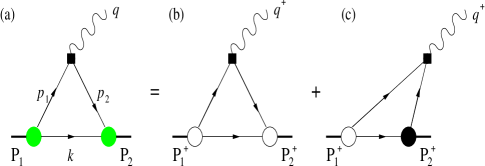
Figure 1: The covariant diagram (a) corresponds to the sum of the LF valence diagram (b) defined in $0<k^{+}<P^{+}_{2}$ region and the nonvalence diagram (c) defined in $P^{+}_{2}<k^{+}<P^{+}_{1}$ region. The large white and black blobs at the meson-quark vertices in (b) and (c) represent the ordinary LF wave functions and the non-wave-function vertex, respectively. The small black box at the quark-gauge boson vertex indicates the insertion of the relevant Wilson operator.

The solvable model, based on the covariant BS model of $(3+1)$-dimensional fermion field theory [9, 14], enables us to derive the transition form factors between pseudoscalar and vector mesons explicitly. The covariant diagram shown in Fig. 1(a) is in general equivalent to the sum of the LF valence diagram [Fig. 1(b)] and the nonvalence diagram [Fig. 1(c)]. The matrix element $\langle J^{\mu}_{h}\rangle_{0(5)}$ obtained from the covariant diagram of Fig. 1(a) is given by

$$\langle J^{\mu}_{h}\rangle_{0(5)}=ig_{1}g_{2}\Lambda^{2}_{1}\Lambda^{2}_{2}\int\frac{d^{4}k}{(2\pi)^{4}}\frac{(S^{\mu}_{h})_{0(5)}}{N_{\Lambda_{1}}N_{1}N_{\bar{q}}N_{2}N_{\Lambda_{2}}},$$ (2)

where $g_{1}$ and $g_{2}$ are the normalization factors which can be fixed by requiring charge form factors of pseudoscalar and vector mesons to be unity at $q^{2}=0$, respectively. To regularize the covariant fermion triangle loop in $(3+1)$ dimensions, we replace the point gauge boson vertex $\gamma^{\mu}(1-\gamma_{5})$ by a non-local (smeared) gauge boson vertex $({\Lambda_{1}}^{2}/N_{\Lambda_{1}})\gamma^{\mu}(1-\gamma_{5})({\Lambda_{2}}^{2}/N_{\Lambda_{2}})$, where $N_{\Lambda_{1}}=p_{1}^{2}-{\Lambda_{1}}^{2}+i\epsilon$ and $N_{\Lambda_{2}}=p_{2}^{2}-{\Lambda_{2}}^{2}+i\epsilon$, and $\Lambda_{1}$ and $\Lambda_{2}$ play the role of momentum cut-offs similar to the Pauli-Villars regularization. The rest of the denominators in Eq. (2) coming from the intermediate fermion propagators in the triangle loop diagram are given by $N_{1}=p_{1}^{2}-{m_{1}}^{2}+i\epsilon$, $N_{\bar{q}}=k^{2}-m^{2}+i\epsilon$, and $N_{2}=p_{2}^{2}-{m_{2}}^{2}+i\epsilon$, where $m_{1}$, $m$, and $m_{2}$ are the masses of the constituents carrying the intermediate four-momenta $p_{1}=P_{1}-k$, $k$, and $p_{2}=P_{2}-k$, respectively.

The trace terms $(S^{\mu}_{h})_{0}$ and $(S^{\mu}_{h})_{5}$ are given by

$$(S^{\mu}_{h})_{0} = {\rm Tr}[(\not\!p_{2}+m_{2})i\sigma^{\mu\nu}q_{\nu}(\not\!p_{1}+m_{1})\gamma_{5}(-\not\!k+m)\epsilon^{*}_{h}\cdot\Gamma],$$

$$(S^{\mu}_{h})_{5} = {\rm Tr}[(\not\!p_{2}+m_{2})i\sigma^{\mu\nu}q_{\nu}\gamma_{5}(\not\!p_{1}+m_{1})\gamma_{5}(-\not\!k+m)\epsilon^{*}_{h}\cdot\Gamma],{}$$ (3)

where the final-state vector meson vertex operator $\Gamma^{\mu}$ is given by

$$\Gamma^{\mu}=\gamma^{\mu}-\frac{(P_{2}-2k)^{\mu}}{D}.$$ (4)

In this work, we shall analyze with the $D$ factor, $D_{\rm cov}(M_{V})=M_{2}+m_{2}+m$, for the explicit comparison between the manifestly covariant calculation and the LF one. However, since the more realistic $D$ factor used in most popular LF quark model is either $D_{\rm cov}(k\cdot P_{2})=[2k\cdot P_{2}+M_{2}(m_{2}+m)-i\epsilon]/M_{2}$ or $D_{\rm LF}(M^{\prime}_{0})=M^{\prime}_{0}+m_{2}+m$ with the invariant mass $M^{\prime}_{0}$ for the final vector meson state, we also discuss the results for both $D_{\rm cov}(k\cdot P_{2})$ and $D_{\rm LF}(M^{\prime}_{0})$ cases.

In the manifestly covariant calculation of Fig. 1(a), we decompose the product of five denominators given in Eq. (2) into a sum of terms containing three propagators. We then use the Feynman parametrization for the three propagators and make a Wick rotation of Eq. (2) in $d=4-2\epsilon$ dimensions to regularize the integral, since otherwise one looses the logarithmically divergent terms in Eq. (2). Following the above procedure (see [16, 18] for more details), one can easily obtain the manifestly covariant form factors $T_{i}(q^{2})(i=1,2,3)$.

Performing the LF calculation of Figs. 1(b) and 1(c) in parallel with the manifestly covariant calculation, we first choose $q^{+}>0$ frame and then take $q^{+}\to 0$ limit to check the existence/absence of the zero-mode contribution to the hadronic matrix element given by Eq. (2). We also use the plus component of the currents to obtain the tensor form factors. While the form factor $T_{1}(q^{2})$ can be obtained from $\langle J^{+}_{h}\rangle_{0}$ with $h=1$, the form factors $T_{2}(q^{2})$ and $T_{3}(q^{2})$ can be obtained from $\langle J^{+}_{h}\rangle_{5}$ with both $h=0$ and $1$. In the reference frame where $q^{+}>0$ and ${\bf P}_{1\perp}=0$, the (timelike) momentum transfer $q^{2}$ is given by

$${}q^{2}=q^{+}q^{-}-{\bf q}^{2}_{\perp}=\Delta\biggl{(}M^{2}_{1}-\frac{M^{2}_{2}}{1-\Delta}\biggr{)}-\frac{{\bf q}^{2}_{\perp}}{1-\Delta},$$ (5)

where $\Delta=q^{+}/P^{+}_{1}$. In this frame, the covariant diagram Fig. 1(a) corresponds to the sum of the LF valence diagram (b) defined in $0<k^{+}<P^{+}_{2}$ region and the nonvalence diagram (c) defined in $P^{+}_{2}<k^{+}<P^{+}_{1}$ region. The large white and black blobs at the meson-quark vertices in (b) and (c) represent the ordinary LF wave functions and the non-wave-function vertex, respectively. The small black box at the quark-gauge boson vertex indicates the insertion of the relevant Wilson operator. We should note that in the $q^{+}\to 0$ (i.e. $\Delta\to 0$) limit, the nonvalence region (i.e. $0<x<\Delta$) of integration shrinks to zero. Thus, if the integrand has a singularity in $p^{-}_{1}\sim 1/x$, the nonvalence region may give a nonvanishing zero mode in the $q^{+}\to 0$ limit. In the LF calculations for the trace terms $(S^{\mu}_{h})_{0(5)}$ in Eq. (3), we separate the on-mass-shell propagating part $S^{\mu}_{\rm on}$ from the off-mass-shell instantaneous part $S^{\mu}_{\rm inst}$, i.e. $S^{\mu}_{h}=(S^{\mu}_{h})^{\rm on}+(S^{\mu}_{h})^{\rm inst}$ via $\not\!p+m=(\not\!p_{\rm on}+m)+\frac{1}{2}\gamma^{+}(p^{-}-p^{-}_{\rm on})$. While the on-mass-shell propagating part $(S^{\mu}_{h})^{\rm on}$ indicates that all three quarks are on their respective mass-shell, i.e. $k^{-}=k^{-}_{\rm on}$ and $p^{-}_{i}=p^{-}_{i\rm on}(i=1,2)$, the instantaneous part $(S^{\mu}_{h})^{\rm inst}$ includes the term proportional to $\delta p_{i}^{-}=p^{-}_{i}-p_{i\rm on}^{-}$ and $\delta k^{-}=k^{-}-k^{-}_{\rm on}$. The relations between the current matrix elements and the form factors in the $q^{+}=0$ [or Drell-Yan(DY)] frame [23] are as follows:

$${}\langle J^{+}_{h=1}\rangle_{0} = 2\sqrt{2}\varepsilon_{+-12}P^{+}_{1}q^{L}T_{1}^{\rm DY}(q^{2}),$$

$$\langle J^{+}_{h=1}\rangle_{5} = -\sqrt{2}P^{+}_{1}q^{L}\biggl{[}T^{\rm DY}_{2}+\frac{q^{2}}{P\cdot q}T^{\rm DY}_{3}\biggr{]},$$

$$\langle J^{+}_{h=0}\rangle_{5} = \frac{q^{2}}{M_{2}}P^{+}_{1}\biggl{[}T^{\rm DY}_{2}-\frac{P\cdot q-q^{2}}{P\cdot q}T^{\rm DY}_{3}\biggr{]},$$ (6)

where $q^{R(L)}=q_{x}\pm iq_{y}$.

In the valence region $0<k^{+}<P^{+}_{2}$ (i.e. $\Delta<x<1$), the pole $k^{-}=k^{-}_{\rm on}=({\bf k}^{2}_{\perp}+m^{2}_{\bar{q}}-i\epsilon)/k^{+}$ (i.e., the spectator quark) is located in the lower half of the complex $k^{-}$-plane. Thus, the Cauchy integration formula for the $k^{-}$ integral in Eq. (2) gives

$$\langle J^{+}_{h}\rangle_{0(5)}=\frac{N}{16\pi^{3}}\int^{1}_{0}\frac{dx}{(1-x)}\int d^{2}{\bf k}_{\perp}\chi_{1}(x,{\bf k}_{\perp})(S^{+}_{h})_{0(5)}\chi_{2}(x,{\bf k^{\prime}}_{\perp}),$$ (7)

where $N=g_{1}g_{2}\Lambda^{2}_{1}\Lambda^{2}_{2}$ and $(S^{+}_{h})_{0(5)}=(S^{+}_{h})^{\rm on}_{0(5)}+(S^{+}_{h})^{\rm inst}_{0(5)}$. The LF vertex functions $\chi_{1}$ and $\chi_{2}$ are given by

$$\chi_{1(2)}(x,{\bf k}^{(\prime)}_{\perp})=\frac{1}{x^{2}(M^{2}_{1(2)}-M^{(\prime)2}_{0})(M^{2}_{1(2)}-M^{(\prime)2}_{\Lambda_{1(2)}})},$$ (8)

where ${\bf k^{\prime}}_{\perp}={\bf k}_{\perp}+(1-x){\bf q}_{\perp}$ and $M^{(^{\prime})2}_{0}=({\bf k}^{(\prime)2}_{\perp}+m^{2})/(1-x)+({\bf k}^{(\prime)2}_{\perp}+m^{2}_{1(2)})/x$ and $M^{(\prime)2}_{\Lambda_{1(2)}}=M^{(\prime)2}_{0}(m_{1(2)}\to\Lambda_{1(2)})$. We note that only the on-mass-shell propagating parts $(S^{+}_{h})^{\rm on}_{0(5)}$ contribute to the valence region in Eq. (7). The valence contributions to the form factors $T_{i}(q^{2})(i=1,2,3)$ in the $q^{+}=0$ frame are obtained as

$$T_{1}^{\rm DY}(q^{2}) = \frac{N}{8\pi^{3}}\int^{1}_{0}\frac{dx}{(1-x)^{2}}\int d^{2}{\bf k}_{\perp}\;\chi_{1}\chi_{2}\biggl{\{}(2x-1){\bf k}^{2}_{\perp}+(1-x){\bf k}_{\perp}\cdot{\bf q}_{\perp}$$ (9)

$$+{\cal A}_{1}{\cal A}_{2}-2(1-x)\frac{({\bf k}_{\perp}\cdot{\bf q}_{\perp})^{2}}{q^{2}}+2(1-x)\frac{(m_{1}+m_{2})}{D}$$

$$\times\biggl{[}{\bf k}^{2}_{\perp}+\frac{({\bf k}_{\perp}\cdot{\bf q}_{\perp})^{2}}{q^{2}}\biggr{]}\biggr{\}},$$

$$T^{\rm DY}_{2}(q^{2}) = \frac{N}{8\pi^{3}}\int^{1}_{0}\frac{dx}{(1-x)^{2}}\int d^{2}{\bf k}_{\perp}\;\chi_{1}\chi_{2}\biggl{\{}{\bf k}^{2}_{\perp}+(2x-1)(1-x){\bf k}_{\perp}\cdot{\bf q}_{\perp}$$ (10)

$$+{\cal A}_{1}{\cal A}_{2}+2(1-x)\frac{({\bf k}_{\perp}\cdot{\bf q}_{\perp})^{2}}{{\bf q}^{2}_{\perp}}-\frac{2(1-x)}{D}[(1-x)q^{2}-{\bf k}_{\perp}\cdot{\bf q}_{\perp}]$$

$$\times\biggl{[}{\cal A}_{1}-(m_{1}+m_{2})\frac{{\bf k}_{\perp}\cdot{\bf q}_{\perp}}{q^{2}}\biggr{]}\biggr{\}}-\frac{q^{2}}{P\cdot q}T^{\rm DY}_{3}(q^{2}),$$

$$T^{\rm DY}_{3}(q^{2}) = \frac{N}{8\pi^{3}}\int^{1}_{0}\frac{dx}{(1-x)^{2}}\int d^{2}{\bf k}_{\perp}\;\chi_{1}\chi_{2}\biggl{\{}{\bf k}^{2}_{\perp}+{\cal A}_{1}(2m-{\cal A}_{2})$$ (11)

$$+(1-x){\bf k}_{\perp}\cdot{\bf q}_{\perp}-2(1-x)\frac{({\bf k}_{\perp}\cdot{\bf q}_{\perp})^{2}}{q^{2}}-2\frac{{\bf k}_{\perp}\cdot{\bf q}_{\perp}}{q^{2}}[{\bf k}^{2}_{\perp}$$

$$+x(1-x)M^{2}_{2}+xm^{2}+(1-x)(m_{1}m+m_{2}m-m_{1}m_{2})]$$

$$-\frac{2}{D}[{\bf k}^{2}_{\perp}+m^{2}-(1-x)^{2}M^{2}_{2}+(1-x){\bf k}_{\perp}\cdot{\bf q}_{\perp}]$$

$$\times\biggl{[}{\cal A}_{1}-(m_{1}+m_{2})\frac{{\bf k}_{\perp}\cdot{\bf q}_{\perp}}{q^{2}}\biggr{]}\biggr{\}},$$

where ${\cal A}_{i}=(1-x)m_{i}+xm(i=1,2)$. When we consider only the simple vector meson vertex $\Gamma^{\mu}_{V}=\gamma^{\mu}$ (i.e. $1/D=0$), our LF results $T^{\rm DY}_{i}(q^{2})(i=1,2,3)$ obtained from the valence contributions in the $q^{+}=0$ frame are exactly the same as the manifestly covariant results. That is, there are no zero-mode contributions to the form factors $T_{i}(q^{2})(i=1,2,3)$. Indeed, our LF results $T^{\rm DY}_{i}(q^{2})(i=1,2,3)$ are also immune to the zero mode even if we include the more realistic $D$ factor such as $D_{\rm cov}(k\cdot P_{2})$ and $D_{\rm LF}(M^{\prime}_{0})$. Only if we use the naive $D$ factor such as $D_{\rm cov}(M_{V})=M_{V}+m_{2}+m$, the zero-mode contribution exists in the matrix element of $\langle J^{+}_{h=0}\rangle_{5}$.

For the completeness of the analysis, we shall identify the zero-mode contribution to $\langle J^{+}_{h=0}\rangle_{5}$ for the $D=D_{\rm cov}(M_{V})$ case. In the nonvalence region $P^{+}_{2}<k^{+}<P^{+}_{1}$ (i.e. $0<x<\Delta$), the poles are at $p^{-}_{1}=p^{-}_{1\rm on}(m_{1})=[m^{2}_{1}+{\bf k}^{2}_{\perp}-i\epsilon]/p^{+}_{1}$ (from the struck quark propagator) and $p^{-}_{1}=p^{-}_{1\rm on}(\Lambda_{1})=[\Lambda^{2}_{1}+{\bf k}^{2}_{\perp}-i\epsilon]/p^{+}_{1}$ (from the smeared quark-gauge-boson vertex), which are located in the upper half of the complex $k^{-}$-plane. For $D=D_{\rm cov}(M_{V})$ case, we find the suspected zero-mode terms, i.e. singular terms proportional to $p^{-}_{1}$ in the off-mass-shell propagator $(S^{+}_{h=0})^{\rm inst}_{5}$ as follows

$$(S^{+}_{h=0})^{\rm Z.M.}_{5}=\lim_{\Delta\to 0}(S^{+}_{h=0})^{\rm inst}_{5}=\frac{4p^{-}_{1}}{M_{2}D}[m_{1}{\bf q}^{2}_{\perp}-(m_{1}+m_{2}){\bf p}_{1\perp}\cdot{\bf q}_{\perp}].$$ (12)

We note that the suspected zero-mode terms $(S^{+}_{h=0})^{\rm Z.M.}_{5}$ in Eq. (12) leads to the nonvanishing zero-mode contribution to $\langle J^{+}_{h=0}\rangle_{5}$ when $D=D_{\rm cov}(M_{V})$ due to the singular behavior $p^{-}_{1}/D_{\rm cov}(M_{V})\sim 1/x$. Following the similar procedure discussed in [16, 18], we can identify the zero-mode operator that is convoluted with the initial- and final-state valence wave functions to generate the zero-mode contribution. Explicitly, the zero-mode contribution $\langle J^{+}_{h=0}\rangle^{\rm Z.M.}_{5}$ or $T_{3}^{\rm Z.M.}=(M_{2}/q^{2})\langle J^{+}_{h=0}\rangle^{\rm Z.M.}_{5}$ can be expressed in terms of the zero-mode operator convoluted with the initial- and final-state LF vertex functions:

$$T_{3}^{\rm Z.M.}(q^{2}) = \frac{N}{8\pi^{3}}\frac{2}{D_{\rm cov}(M_{V})}\int^{1}_{0}\frac{dx}{(1-x)}\int d^{2}{\bf k}_{\perp}\chi_{1}\chi_{2}$$ (13)

$$\times\biggl{\{}(m_{1}+m_{2})\biggl{[}A^{(1)}_{2}Z_{2}+\frac{q\cdot P}{q^{2}}A^{(2)}_{1}\biggr{]}-m_{1}Z_{2}\biggr{\}},$$

where $A^{(1)}_{2}$, $A^{(2)}_{1}$, and $Z_{2}$ are given by [13, 16]

$$A^{(1)}_{2}=\frac{x}{2}+\frac{{\bf k}_{\perp}\cdot{\bf q}_{\perp}}{q^{2}},\;A^{(2)}_{1}=-{\bf k}^{2}_{\perp}-\frac{({\bf k}_{\perp}\cdot{\bf q}_{\perp})^{2}}{q^{2}},$$

$$Z_{2}=x(M^{2}_{1}-M^{2}_{0})+m^{2}_{1}-m^{2}+(1-2x)M^{2}_{1}-[q^{2}+q\cdot P]\frac{{\bf k_{\perp}\cdot{\bf q}_{\perp}}}{q^{2}}.$$

By adding $T_{3}^{\rm Z.M.}(q^{2})$ to $T_{3}^{\rm DY}(q^{2})$ in Eqs. (10) and  (11), i.e. $T_{3}^{\rm Full}(q^{2})=T_{3}^{\rm DY}(q^{2})+T_{3}^{\rm Z.M.}(q^{2})$, we confirm that our LF results for the form factors $T_{2}$ and $T_{3}$ are in an exact agreement with the manifestly covariant results for the $D=D_{\rm cov}(M_{V})$ case.

However, $T_{3}^{\rm Z.M.}(q^{2})$ vanishes when $D=D_{\rm cov}(k\cdot P_{2})$ or $D_{\rm LF}(M^{\prime}_{0})$ is used. This can be easily seen from the power counting rule for $x$ (or $p^{-}_{1}$) in $x\to 0$ limit. Note that $D_{\rm cov}(k\cdot P_{2})\sim x^{-1}$ and $D_{\rm LF}(M^{\prime}_{0})\sim x^{-1/2}$ while $p^{-}_{1}\sim x^{-1}$ in the same $x\to 0$ limit. Since $p^{-}_{1}/D_{\rm cov}(k\cdot P_{2})\sim x^{0}$ and $p^{-}_{1}/D_{\rm LF}(M^{\prime}_{0})\sim x^{-1/2}$, the case of $D_{\rm cov}(k\cdot P_{2})$ or $D_{\rm LF}(M^{\prime}_{0})$ provides less singular behavior than the case of $D_{\rm cov}(M_{V})$. More detailed power counting rule for the longitudinal momentum fraction can be found in [16, 17, 18]. Therefore, as far as the $D_{\rm LF}(M^{\prime}_{0})$ or $D_{\rm cov}(k\cdot P_{2})$ is used in LFQM, there are no zero-mode contributions to the tensor form factors $T_{i}(q^{2})(i=1,2,3)$ and the form factors given by Eqs. (9)-(11) are the correct LF tensor form factors.

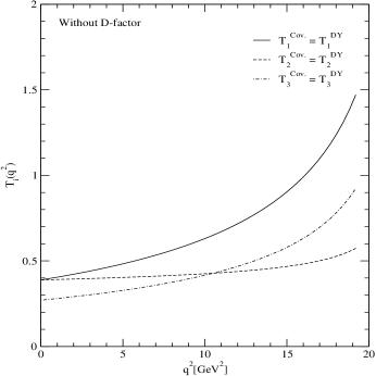
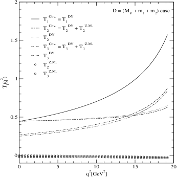
Figure 2: The tensor form factors $T_{i}(q^{2})(i=1,2,3)$ for $B\to K^{*}$ transition for the simple vector meson vertex $\Gamma^{\mu}=\gamma^{\mu}$ case (i.e. without the $D$ factor) and for $\Gamma^{\mu}=\gamma^{\mu}-(P_{2}-2k)^{\mu}/D$ with the $D=D_{\rm cov}(M_{V})$, respectively.

In Fig. 2, we show both the manifestly covariant and the LF results of the tensor form factors $T_{i}(q^{2})(i=1,2,3)$ for the rare $B\to K^{*}\ell^{+}\ell^{-}$ transition obtained from the exactly solvable covariant BS model of fermion field theory. The used model parameters for $B$ and $K^{*}$ mesons are $m_{b}=4.9$ GeV, $m_{s}=0.5$ GeV, $m_{u(d)}=0.43$ GeV, $\Lambda_{1}=10$ GeV, $\Lambda_{2}=2.5$ GeV, $g_{1}=5.13$, and $g_{2}=3.2$. The left and right panels of Fig. 2 are the results for the simple vector meson vertex $\Gamma^{\mu}=\gamma^{\mu}$ case (i.e. $1/D=0$) and for $\Gamma^{\mu}=\gamma^{\mu}-(P_{2}-2k)^{\mu}/D$ with $D=D_{\rm cov}(M_{V})$, respectively. Our LF results $T^{\rm DY}_{i}(q^{2})(i=1,2,3)$ obtained from the $q^{+}=0$ frame are analytically continued to the timelike $q^{2}>0$ region by changing ${\bf q}^{2}_{\perp}$ to $-q^{2}$ in the form factor. The results for the more realistic covariant vertex with $D=D_{\rm cov}(k\cdot P_{2})$ are basically the same as those for the simple vertex case although the quantitative behaviors are slightly different from each other, i.e., the LF tensor form factors $T_{i}^{\rm DY}(q^{2})$ given by Eqs. (9)-(10) with $D=D_{\rm cov}(k\cdot P_{2})$ are exact results without encountering the zero-mode contribution. For the $D=D_{\rm LF}(M^{\prime}_{0})$ case, although we do not know how to compute the nonvalence diagram, we can still use our counting rule for the longitudinal momentum fraction factors, i.e. $p^{-}_{1}/D_{\rm LF}(M^{\prime}_{0})\to(1/x)^{1/2}$ as $\Delta\to 0$, to check the existence of the zero mode. As we discussed, the zero-mode contribution from $p^{-}_{1}/D_{\rm LF}(M^{\prime}_{0})$ does not exist as in the case of $D=D_{\rm cov}(k\cdot P_{2})$.

In Table 1, we summarize our findings of the existence/absence of the zero-mode contribution to the hadronic form factors ($g,a_{\pm},f$) [17, 18] and $T_{i}(i=1,2,3)$ for the rare $P\to V\ell^{+}\ell^{-}$ decays depending on the components of the weak currents $J^{\mu}_{V-A}$, polarization vector $\epsilon^{*}_{h}$ of the vector meson, and various $D$ factors in $\Gamma^{\mu}_{\rm V}$. Since our findings of the existence/absence of the zero mode are based on the method of power counting, our conclusion applies to other methods of regularization as far as the regularization doesn’t change the power counting in the form factor calculation. For example, as discussed by Jaus in Ref. [13], some other multipole type ansatz in the method of regularization wouldn’t change the conclusion drawn by our monopole type ansatz. This may exemplify the benefit of our method to remove any unnecessary caution regarding on the possible zero-mode contribution in the hadron phenomenology by correctly pinning down its existence/absence.

Table 1: The existence ($\rm O$) or absence ($\rm X$) of the zero-mode contribution to the form factors for the rare $P\to V\ell^{+}\ell^{-}$ decays depending on the components of the currents $J^{\mu}$, polarization vector $\epsilon^{*}_{h}$ of the vector meson, and various $D$ factors in $\Gamma^{\mu}_{\rm V}$.

	$g$	$a_{+}$	$a_{-}$	$f$	$T_{1}$	$T_{2}$	$T_{3}$
$\langle J^{\mu}_{h}\rangle$	$\langle J^{+}_{1}\rangle_{V}$	$\langle J^{+}_{1}\rangle_{A}$	$\langle J^{+}_{0,1}\rangle_{A}$,$\langle J^{\perp}_{1}\rangle_{A}$	$\langle J^{+}_{0,1}\rangle_{A}$	$\langle J^{+}_{1}\rangle_{0}$	$\langle J^{+}_{0,1}\rangle_{5}$	$\langle J^{+}_{0,1}\rangle_{5}$
$\Gamma^{\mu}_{\rm V}=\gamma^{\mu}$	$\rm X$	$\rm X$	$\rm O$	$\rm X$	$\rm X$	$\rm X$	$\rm X$
$\Gamma^{\mu}_{\rm V}[D_{\rm cov}(M_{V})]$	$\rm X$	$\rm X$	$\rm O$	$\rm O$	$\rm X$	$\rm O$	$\rm O$
$\Gamma^{\mu}_{\rm V}[D_{\rm cov}(k\cdot P_{2})]$	$\rm X$	$\rm X$	$\rm O$	$\rm X$	$\rm X$	$\rm X$	$\rm X$
$\Gamma^{\mu}_{\rm V}[D_{\rm LF}(M^{\prime}_{0})]$	$\rm X$	$\rm X$	$\rm O$	$\rm X$	$\rm X$	$\rm X$	$\rm X$

In this work, we have analyzed the zero-mode contribution to the tensor form factors for the rare $P\to V\ell^{+}\ell^{-}$ decays. For the phenomenologically accessible vector meson vertex $\Gamma^{\mu}_{\rm V}=\gamma^{\mu}-(P_{2}-k)^{\mu}/D$, we discussed the three typical cases of the $D$ factor which also may be classified by the differences in the power counting of the LF energy (or longitudinal momentum fraction $x$) $p^{-}_{1}\sim 1/x$, i.e.: (1) $D_{\rm cov}(M_{V})=M_{V}+m_{2}+m\sim(1/x)^{0}$, (2) $D_{\rm cov}(k\cdot P_{2})=[2k\cdot P_{2}+M_{2}(m_{2}+m)-i\epsilon]/M_{2}\sim(1/x)^{1}$, and (3) $D_{\rm LF}(M^{\prime}_{0})=M^{\prime}_{0}+m_{2}+m\sim(1/x)^{1/2}$. Our main idea to obtain the transition form factors is first to find if the zero-mode contribution exists or not for the given form factor using the power counting method. If it exists, then the separation of the on-mass-shell propagating part from the off-mass-shell part is useful since the latter is responsible for the zero-mode contribution. We found that the form factor $T_{1}(q^{2})$ is immune to the zero-mode contribution in all three cases of the $D$ factors. However, for the form factors $T_{2}(q^{2})$ and $T_{3}(q^{2})$, while the zero-mode contribution exists in the $D_{\rm cov}(M_{V})$ case, the other two cases such as $D_{\rm cov}(k\cdot P_{2})$ and $D_{\rm LF}(M^{\prime}_{0})$ are immune to the zero-mode contribution. We also should note that the zero-mode contribution does not exist in the simple vector meson vertex $\Gamma^{\mu}=\gamma^{\mu}$ (i.e. $1/D=0$ case).

All of these findings stem from the fact that the zero-mode contribution from the $D$ factor is absent if the denominator $D$ of the vector meson vertex $\Gamma^{\mu}=\gamma^{\mu}-(P_{2}-k)^{\mu}/D$ contains the term proportional to the LF energy (or longitudinal momentum fraction $x$) $(p^{-}_{1})^{n}\sim(1/x)^{n}$ with the power $n>0$. Since the phenomenologically accessible LFQM satisfies this condition $n>0$, only the valence contributions to the three weak form factors ($g,a_{+},f$) and the three tensor form factors $T_{i}(q^{2})(i=1,2,3)$ obtained in the $q^{+}=0$ frame for the analysis of the rare $P\to V\ell^{+}\ell^{-}$ decays are sufficient to provide the full results of the LFQM. Although the form factor $a_{-}(q^{2})$ receives the zero-mode contribution, it comes only from the simple vertex $\gamma^{\mu}$ term but not from the $D$ factor satisfying the condition $n>0$. In this case, we were able to obtain the correct zero-mode operator that is convoluted with the initial- and final-state LF wave functions [18]. Our analyses of zero-mode contribution can at least assure the Lorentz invariance of the hadron form factors in the exclusive processes that we have considered up to now. This certainly benefits the hadron phenomenology and the application to the more realistic LFQM analysis for various semileptonic and rare $P\to V$ decays is underway.

References

[1] N. Cabibbo, Phys. Rev. Lett. 10 (1963) 531 ;
M. Kobayashi and T. Maskawa, Prog. Theor. Phys. 49 (1973) 652.
[2] B. Grinstein, M. B. Wise and M. J. Savage,
Nucl. Phys. B 319 (1989) 271 ; A. J. Buras and M. Mnz,
Phys. Rev. D 52 (1995) 186 ; M. Misiak, Nucl. Phys. B 393 (1993) 23 ;
T. Inami and C. S. Lim, Prog. Theor. Phys. 65 (1981) 297;
A. Ali, T. Mannel and T. Morozumi, Phys. Lett. B 273 (1991) 505 ;
C. S. Kim, T. Morozumi, and A. I. Sanda, Phys. Rev. D 56 (1997) 7240 .
[3] S. J. Brodsky, H.-C. Pauli, and S. S. Pinsky,
Phys. Rep. 301 (1998) 299.
[4] M. V. Terent’ev, Yad. Fiz. 24 (1976) 207[Sov. J. Nucl.
Phys. 24 (1976) 106].
[5] Z. Dziembowsky and L. Mankiewicz, Phys. Rev. Lett. 58 (1987) 2175 ;
Z. Dziembowsky, Phys. Rev. D 37 (1988) 778 .
[6] P. L. Chung, F. Coester, and W. N. Polyzou,
Phys. Lett. B 205 (1988) 545 .
[7] C.-R. Ji and S.R. Cotanch, Phys. Rev. D 41 (1990) 2319 ;
C.-R. Ji, P.L. Chung, and S.R. Cotanch, Phys. Rev. D 45 (1992) 4214 .
[8] W. Jaus, Phys. Rev. D 41 (1990) 3394 ;
Phys. Rev. D 44 (1991) 2851 .
[9] J.P.B.C. de Melo and T.Frederico,
Phys. Rev. C 55 (1997) 2043 ; J.P.B.C. de Melo, T.Frederico, E. Pace,
and G. Salme, Phys. Lett. B 581 (2004) 75 ; Phys. Rev. D 73 (2006) 074013 .
[10] H.-M. Choi and C.-R. Ji,
Phys. Rev. D 59 (1999) 074015 ; Phys. Lett. B 460 (1999) 461 ;
C.-R. Ji and H.-M. Choi, Phys. Lett. B 513 (2001) 330 .
[11] H.-Y. Cheng, C.-K. Chua, and C.-W. Hwang,
Phys. Rev. D 69 (2004) 074025 ; H.-Y. Cheng and C.-K. Chua,
Phys. Rev. D 81 (2010) 114006 .
[12] M. Burkardt, Phys. Rev. D 47 (1993) 4628 ;
S. J. Brodsky and D. S. Hwang,
Nucl. Phys. B 543 (1998) 239 ;
J.P.B.C. de Melo, J.H.O. Sales, T. Frederico, and P.U. Sauer,
Nucl. Phys. A 631 (1998) 574c ;
H.-M. Choi and C.-R. Ji,
Phys. Rev. D 58 (1998) 071901(R) .
[13] W. Jaus, Phys. Rev. D 60 (1999) 054026 ;
Phys. Rev. D 67 (2003) 094010 .
[14] B. L. G. Bakker, H.-M. Choi, and C.-R. Ji,
Phys. Rev. D 65 (2002) 116001 ;
Phys. Rev. D 67 (2003) 113007 .
[15] H.-M. Choi, and C.-R. Ji,
Phys. Rev. D 70 (2004) 053015 .
[16] H.-M. Choi and C.-R. Ji, Phys. Rev. D 80 (2009) 054016 ;
H.-M. Choi, Phys. Rev. D 81 (2010) 054003 .
[17] H.-M. Choi and C.-R. Ji, Phys. Rev. D 72 (2005) 013004 .
[18] H.-M. Choi and C.-R. Ji, arXiv:1007.2502 [hep-ph].
[19] H.-M. Choi, Phys. Rev. D 75 (2007) 073016 ;
J. Korean Phys. Soc. 53, 1205 (2008).
[20] C.-W. Hwang and Z.-T. Wei, J. Phys. G 34 (2007) 687 .
[21] W. Qian and B.-Q. Ma, Phys. Rev. D 78 (2008) 074002 ;
W. Wang, Y.-L. Shen and C.-D. Lu, Phys. Rev. D 79 (2009) 054012 .
[22] T. Altomari and L. Wolfenstein,
Phys. Rev. D 37 (1988) 681 .
[23] S. D. Drell and T. M. Yan, Phys. Rev. Lett. 24 (1970) 181 ;
G. West, Phys. Rev. Lett. 24 (1970) 1206 .