Exact crossover Green function in the two-channel and two-impurity Kondo models

Abstract

Symmetry-breaking perturbations destabilize the critical points of the two-channel and two-impurity Kondo models, thereby leading to a crossover from non-Fermi liquid behavior to standard Fermi liquid physics. Here we use an analogy between this crossover and one occurring in the boundary Ising model to calculate the full crossover Green function analytically. In remarkable agreement with our numerical renormalization group calculations, the single exact function applies for an arbitrary mixture of the relevant perturbations in each model. This rich behavior resulting from finite channel asymmetry, inter-lead charge transfer and/or magnetic field should be observable in quantum dot or tunneling experiments.

The most basic quantum impurity model exhibiting non-Fermi liquid (NFL) behavior is arguably the two-channel Kondo (2CK) model NozieresBlandin , describing the symmetric antiferromagnetic coupling of a local spin-$\tfrac{1}{2}$ impurity to two equivalent but independent conduction channels. The resulting ground state possesses various intriguing properties, including notably a residual entropy s of $\tfrac{1}{2}k_{B}\ln(2)$ and conductance that approaches its $T=0$ value as $\sqrt{T}$ (for a review see Ref. [rev:cox_zaw, ]).

The same behaviour is predicted at the critical point of the two-impurity Kondo (2IK) model CFT2IKM . The tendency to form a trivial local singlet state is favoured by an exchange coupling acting directly between the impurities; while the coupling of each impurity to its own metallic lead favours separate single-channel Kondo screening. The resulting competition gives rise to a critical point that is closely related to the 2CK state.

The central difficulty in realizing experimentally the NFL physics of either model is the extreme delicacy of the 2CK fixed point (FP) to various symmetry-breaking perturbations. Channel asymmetry, magnetic field and inter-lead charge transfer processes all destabilise the 2CK FP and destroy NFL behaviour in both 2CK and 2IK models.

Tremendous efforts have been made to suppress these relevant perturbations in order to observe the characteristic NFL behaviour in a real 2CK device. The quantum dot system realized recently in Ref. Potok07 shows unambiguous signatures associated with flow to the 2CK FP. But in any real system, the presence of destabilising perturbations is totally inevitable, leading ultimately to a crossover from NFL behaviour to standard Fermi liquid physics on the lowest energy scales.

In this Letter we demonstrate that an arbitrary mixture of the relevant perturbations in either the 2CK or 2IK model leads to low-energy behaviour of the impurity Green function that is wholly characteristic of the incipient 2CK state, and which can not be extracted from the Bethe-ansatz solution andrei . We derive a single exact function to describe this crossover, which agrees perfectly with our full numerical renormalization group (NRG) calculations for both models, and whose rich behaviour should be directly observable in quantum dot or tunneling experiments.

Models and perturbations.– We consider the standard 2CK and 2IK models,

$$H_{2CK}=H_{0}+ J\vec{S}\cdot(\vec{s}_{0L}+\vec{s}_{0R})+\delta H_{2CK},$$ (1)

$$H_{2IK}=H_{0}+ J(\vec{S}_{L}\cdot\vec{s}_{0L}+\vec{S}_{R}\cdot\vec{s}_{0R})+K\vec{S}_{L}\cdot\vec{S}_{R}+\delta H_{2IK},$$

where $H_{0}=\sum_{\alpha,k}\epsilon_{k}^{\phantom{\dagger}}\psi_{k}^{\dagger\sigma\alpha}\psi^{\phantom{\dagger}}_{k\sigma\alpha}$ describes two free conduction electron channels $\alpha=L/R$, with spin density $\vec{s}_{0\alpha}=\sum_{\sigma\sigma^{\prime}}\psi_{0}^{\dagger\sigma\alpha}(\tfrac{1}{2}\vec{\sigma}_{\sigma\sigma^{\prime}})\psi^{\phantom{\dagger}}_{0\sigma^{\prime}\alpha}$ (and $\psi_{0}^{\dagger\sigma\alpha}=\sum_{k}\psi_{k}^{\dagger\sigma\alpha}$) coupled to one spin-$\tfrac{1}{2}$ impurity $\vec{S}$ (2CK) or two impurity spins $\vec{S}_{L,R}$ (2IK). For $\delta H_{2CK}=0$, the ground state of $H_{2CK}$ is described by the 2CK FP. Likewise, a critical inter-impurity coupling $K_{c}$ can be found such that the ground state of $H_{2IK}$ is similarly described by the 2CK FP for $\delta H_{2IK}=0$.

Relevant perturbations to each model have been identified from conformal field theory (CFT) CFT2CK ; CFT2IKM and are generically present in experiment. Specifically,

$$\delta H_{2CK}=\sum_{\ell=x,y,z}\Delta_{\ell}\sum_{\alpha,\beta}\sum_{\sigma\sigma^{\prime}}\psi_{0}^{\dagger\sigma\alpha}(\tfrac{1}{2}\vec{\sigma}_{\sigma\sigma^{\prime}}\tau_{\alpha\beta}^{\ell})\psi_{0\sigma^{\prime}\beta}\cdot\vec{S}+\vec{B}\cdot\vec{S},$$ (3)

describes $L/R$ channel asymmetry in the 2CK model for $\Delta_{z}\neq 0$, while charge transfer between the leads is embodied in the $\Delta_{x}$ and $\Delta_{y}$ components of the first term [here $\vec{\tau}\leavevmode\nobreak\ (\vec{\sigma})$ are the Pauli matrices in the channel (spin) sector]. The second term describes a magnetic field acting on the impurity. For the 2IK model, the critical point is destabilized by finite $(K_{c}-K)$, and also through

$$\delta H_{2IK}=\sum_{\sigma}(V_{LR}\psi_{0}^{\dagger\sigma L}\psi_{0\sigma R}+\text{H.c.})+\vec{B}_{s}\cdot(\vec{S}_{L}-\vec{S}_{R}),$$ (4)

where $V_{LR}$ describes electron tunneling between the leads and $\vec{B}_{s}$ the application of a staggered magnetic field.

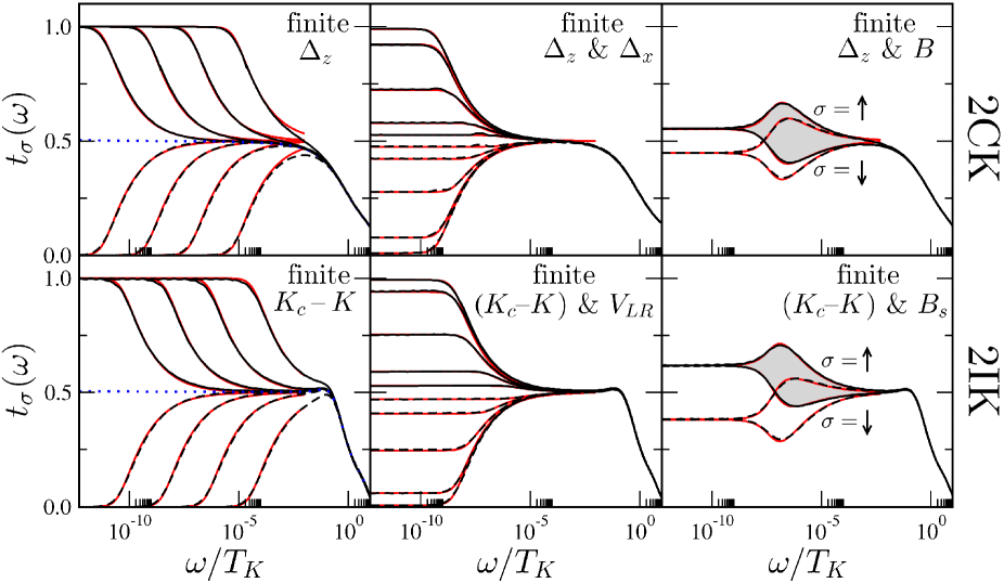
Figure 1: Spectrum $t_{\sigma}(\omega)$ vs. $\omega/T_{K}$ for the 2CK model (upper panels) and the 2IK model (lower panels) at $T=0$ in the presence of various perturbations. Entire frequency dependence calculated by NRG (black lines); low-energy $\omega\ll T_{K}$ behaviour in each case compared with exact crossover function Eq. (7) (red lines). All results presented for $\nu J=0.25$. Left: effect of channel asymmetry $\Delta_{z}\neq 0$ (2CK) or deviation from critical coupling $(K_{c}-K)\neq 0$ (2IK). Specifically, $4\nu\Delta_{z}=(K_{c}-K)/D=\pm 10^{-n}$ (with $\pm$ for solid and dashed lines, respectively), and $n=3,\tfrac{7}{2},4,\tfrac{9}{2},5$ in order of decreasing $T^{*}$, approaching successively the limit $\Delta_{z}=(K_{c}-K)=0$ (dotted line). Centre: effect of including also finite left/right tunneling, $\Delta_{x}\neq 0$ (2CK) or $V_{LR}\neq 0$ (2IK). Shown for fixed finite $4\nu\Delta_{z}=(K_{c}-K)/D=\pm 10^{-5}$ with $5\Delta_{x}/|\Delta_{z}|=2D\nu V_{LR}/|K_{c}-K|=10^{-m}$ with $m=2,\tfrac{3}{2},1,\tfrac{1}{2},0$, successively approaching $t_{\sigma}(0)=\tfrac{1}{2}$ from above [solid lines; $\Delta_{z},(K_{c}-K)>0$] and from below [dashed lines; $\Delta_{z},(K_{c}-K)<0$]. Right: effect of including finite magnetic field. Shown again for $4\nu\Delta_{z}=(K_{c}-K)/D=\pm 10^{-5}$, but now with $B/4D\nu|\Delta_{z}|=B_{s}/|K_{c}-K|=10^{1/2}$. As before, solid lines for $\Delta_{z},(K_{c}-K)>0$ and dashed lines for $\Delta_{z},(K_{c}-K)<0$, with both $\sigma=\uparrow$ and $\downarrow$ spectra shown. Excellent agreement between NRG data and analytic curves obtained in all cases from a single set of fitting parameters for each model: $c_{T}=96$ and $c_{B}=0.04$ for 2CK; while $c_{T}=0.63$, $c_{V}=2.4$, $c_{B}=1.3$ for 2IK.

These perturbations generate a new energy scale, $T^{*}$, characterizing the flow away from the 2CK FP, and toward the Fermi liquid (FL) FP. Signatures of this crossover appear in the energy-resolved local density of states, since inelastic scattering ceases at energies $\ll T^{*}$ where the impurity degrees of freedom are quenched. Indeed, the $dI/dV$ conductance through a quantum dot asymmetrically coupled to source and drain leads at zero temperature is related asymmetric to the scattering $T$-matrix: $dI/dV\propto\sum_{\sigma=\uparrow,\downarrow}[-\pi\nu{\rm{Im}}T_{L\sigma}(eV)]$, where $\nu$ is the lead density of states per spin and $V$ the source-drain voltage. The Green function is given by

$$G^{\alpha\sigma}_{kk^{\prime}}(\omega)=G_{k}^{0}(\omega)\delta_{kk^{\prime}}+G_{k}^{0}(\omega)T_{\alpha\sigma}(\omega)G_{k^{\prime}}^{0}(\omega),$$ (5)

with $G_{k}^{0}(\omega)=(\omega-\epsilon_{k}+i0^{+})^{-1}$. Conductance measurements of the 2CK device of Ref. Potok07 or in the proposed 2IK setup of Ref. Zarand2006 thus yield access to the $T$-matrix and hence the full Green function. Our goal here is to calculate the quantity $t_{\sigma}(\omega)=-\pi\nu{\rm{Im}}T_{L\sigma}(\omega)$ exactly and numerically for the 2CK and 2IK models in the presence of symmetry-breaking perturbations described by Eqs. (1)–(4).

Results.– Preempting the technical discussion of the next section, we present now the key results of the Letter. Heralding renormalization group flow to the stable FL FP, the low-energy crossover scale is given generically by

$$T^{*}=c_{T}\lambda^{2},$$ (6)

where $\lambda^{2}=\sum_{j=1}^{8}\lambda_{j}^{2}$ (and $\{\lambda_{4},\lambda_{5},\lambda_{6}\}=\{\lambda_{B}^{x},\lambda_{B}^{y},\lambda_{B}^{z}\}$). For the 2CK model, $\lambda_{1}=\nu\Delta_{z}\sqrt{T_{K}}$, $\lambda_{2,3}=c_{V}\nu\Delta_{x,y}\sqrt{T_{K}}$ and $\vec{\lambda}_{B}=c_{B}\vec{B}/\sqrt{T_{K}}$; while for 2IK, $\lambda_{1}=(K_{c}-K)/\sqrt{T_{K}}$, $\lambda_{2}+i\lambda_{3}=c_{V}\sqrt{T_{K}}\nu V_{LR}$, and $\vec{\lambda}_{B}=c_{B}\vec{B}_{s}/\sqrt{T_{K}}$. Here $c_{T},c_{V},c_{B}=\mathcal{O}(1)$ are fitting parameters which depend on the model and on $J$, and $T_{K}\propto e^{-\frac{1}{\nu J}}$ is the Kondo temperatre. The perturbations associated with coupling constants $\lambda_{7}$ and $\lambda_{8}$ do not conserve total charge CFT2CK ; CFT2IKM , so are ignored.

In the simplest case of channel anisotropy in the 2CK model, the result $T^{*}\propto(\Delta_{z})^{2}$ has long been established rev:cox_zaw . The extension to finite $\lambda_{1},\lambda_{2},\lambda_{3}\neq 0$ follows by trivial rotation of the bare Hamiltonian in $\vec{\tau}$-space, implying directly that $T^{*}\propto(\Delta_{x})^{2}+(\Delta_{y})^{2}+(\Delta_{z})^{2}$, and hence $c_{V}=1$ for the 2CK model. However, the low-energy effective Hamiltonian for both 2CK and 2IK models possesses a larger SO$(8)$ emergent symmetry that permits a similar rotation, yielding the generalization, Eq. (6). Importantly, we show that the same rotation can also be exploited to obtain a single zero temperature Green function for the crossover. Our exact result for the $T$-matrix is

$$2\pi i\nu T_{\alpha\sigma}(\omega)=1-S_{\alpha\sigma}\mathcal{G}\left(\omega/T^{*}\right),$$ (7)

where $\mathcal{G}(x)=\frac{2}{\pi}K\left[ix\right]$, $K[x]$ is the complete elliptic integral of the first kind, yielding asymptotically $\mathcal{G}[x]=1+ix/4-(3x/8)^{2}+\mathcal{O}(x^{3})$ for $x\ll 1$; and $\mathcal{G}[x]=\frac{\sqrt{i}}{2\pi}(\log[256x^{2}]-i\pi)x^{-1/2}$ for $x\gg 1$. $S_{\alpha\sigma}$ is the FL S-matrix, containing phase shift information, given by

$$S^{2CK}_{\alpha\sigma}=(-\alpha\lambda_{1}+i\sigma\lambda_{B}^{z})/\lambda=\alpha S^{2IK}_{\alpha\sigma},$$ (8)

with $\sigma=\pm 1$ for spins $\uparrow/\downarrow$ and $\alpha=\pm 1$ for channel $L/R$, such that $t_{\sigma}(0)=\frac{1}{2}-\frac{1}{2}{\rm{Re}}S_{L\sigma}$ (and we have used $\vec{\lambda}_{B}\parallel\hat{z}$).

Rich physical behaviour is obtained when combinations of the relevant perturbations are applied. We now discuss relevant and representative cases of the general and exact formula, Eq. (7), valid in the crossover regime $|\omega|\ll T_{K}$. We also employ the NRG technique (for a review, see Ref. nrg:rev ), which can be used to determine accurately $t_{\sigma}(\omega)$ on all energy scales, for both 2CK and 2IK models in the presence of any perturbation. Here we focus on the low-energy behaviour where comparison can be made to the exact results. All symmetries of the problem are exploited, and $N_{s}=6000$ states are retained at each iteration. The leads of width $2D$ are assumed to have a uniform density of states $\nu=1/(2D)$, and are discretized logarithmically nrg:rev .

NRG data and exact results are presented in Fig. 1, with parameters given in the caption. $t_{\sigma}(\omega)$ vs. $\omega/T_{K}$ is plotted for the 2CK model (upper panels) and the 2IK model (lower panels) in the presence of various perturbations. In the left panels, finite $\lambda_{1}$ is considered (channel asymmetry for the 2CK model, and detuning of the inter-impurity coupling in the 2IK model). Precisely at the 2CK FP, $\lambda=0$, $S_{\alpha\sigma}=0$ CFT2CK ; CFT2IKM , and hence $t_{\sigma}(\omega)=\tfrac{1}{2}$ for $|\omega|\ll T_{K}$. But for $\lambda_{1}\neq 0$ one immediately obtains $|t_{\sigma}(\omega)-\tfrac{1}{2}|\sim|\omega/T^{*}|^{-1/2}$ for $T^{*}\ll|\omega|\ll T_{K}$, while for $|\omega|\ll T^{*}$, the classic quadratic approach to the FL FP is given asymptotically by $|t_{\sigma}(\omega)-t_{\sigma}(0)|\sim(\omega/T^{*})^{2}$, with $t_{\sigma}=1$ (solid lines: $\lambda_{1}>0$) or $t_{\sigma}=0$ (dashed lines: $\lambda_{1}<0$) being obtained at $\omega=0$. This full lineshape was likewise obtained numerically for example in Ref. Zarand2006, for the 2IK model, or for the 2CK model Toth ; borda and related odd-impurity chains in Ref. akm:oddimp . The exact crossover function, Eq. (7), is plotted as the red line in each case, showing remarkable agreement for $|\omega|\ll T_{K}$.

The effect of including also left/right charge transfer terms (finite $\lambda_{2}$) is shown in the centre panels ($\lambda_{1}$ now being kept fixed). As $\lambda_{2}$ increases, the $\omega\ll T_{K}$ lineshapes seen in the left panels of Fig. 1 undergo a simple rescaling $t_{\sigma}(\omega)\to\frac{1}{2}+\left|\frac{\lambda_{1}}{\lambda}\right|[t_{\sigma}(\omega)-\frac{1}{2}]$ and eventually for $|\lambda_{2}|\gg|\lambda_{1}|$ they completely flatten. In the 2CK model, the resulting form of $t_{\sigma}(\omega)$ is readily understood: rotation in $\vec{\tau}$-space allows the Hamiltonian to be written in terms of $\Delta_{z}$ only — but $t_{\sigma}(\omega)$ is then a weighted combination of the $\Delta_{z}>0$ and $\Delta_{z}<0$ spectra shown in the left panels. That the same behaviour is observed in the 2IK model (lower-centre panel) is a deeply non-trivial result however. There is no symmetry of the bare Hamiltonian that permits this rotation; rather, it is the result of an emergent symmetry. In both cases, the crossover function is described perfectly by Eq. (7).

Finally, we consider the effect of applying a magnetic field (finite $\lambda_{B}^{z}$). In the absence of other perturbations, $\text{Re}S_{\alpha\sigma}=0$, and hence $t_{\uparrow}(0)=t_{\downarrow}(0)=\tfrac{1}{2}$ (consistent with a $\pi/4$ phase shift pustilnik04 ). Indeed, $t_{\sigma}(\omega)=\tfrac{1}{2}$ for $T^{*}\ll|\omega|\ll T_{K}$ since the system is near the 2CK FP. However, the impurity magnetization $M\sim B^{z}$ for the 2CK model (or staggered magnetization $M_{s}\sim B^{z}_{s}$ in the 2IK model); thus $t_{\uparrow}(\omega)\neq t_{\downarrow}(\omega)$ since $M\propto\int_{-\infty}^{0}\text{d}\omega[t_{\uparrow}(\omega)-t_{\downarrow}(\omega)]\neq 0$. For finite (staggered) magnetization therefore, the ‘up’ and ‘down’ spectra must deviate at finite frequency: a ‘pocket’ opens between the curves at $|\omega|\sim T^{*}$, whose area is proportional to the (staggered) magnetization. This behavior is observed in the right panels of Fig. 1, where a fixed $\lambda_{1}$ is also included.

For $|\omega|\ll T^{*}$, we find a linear approach to the FL FP, $t_{\sigma}(\omega)-t_{\sigma}(0)=\frac{\sigma\lambda_{B}^{z}}{8\lambda}\frac{\omega}{T^{*}}+\mathcal{O}\left(\frac{\omega^{2}}{{T^{*}}^{2}}\right)$, rather than the quadratic dependence usually associated with FL theory. However, this result is a perfectly natural consequence of the complex scattering matrix $S_{\alpha\sigma}$. $t_{\sigma}(\omega)$ comprises contributions from both imaginary and real parts of the complex function $\mathcal{G}(\omega/T^{*})$ in Eq. (7), the latter of which contains a leading linear term. It is this contribution that of course dominates the low-$|\omega|$ behaviour of $t_{\sigma}(\omega)$ in the presence of the magnetic field. Again, there is excellent agreement between the NRG data and the exact results across the entire frequency range $|\omega|\ll T_{K}$. We finally note that the conductance is obtained by averaging $\sigma=\uparrow$ and $\downarrow$ contributions; the imaginary part of $S_{\alpha\sigma}$ thus cancels by Eq. (8), and the characteristic ‘hump’ observed in $t_{\sigma}(\omega)$ is absent in $dI/dV$. In consequence, $dI/dV\sim(eV)^{2}$ for $eV\ll T^{*}$ at finite fields. We now sketch the derivation of Eqs. (7) and (8).

Analytic crossover function at $K\neq K_{c}$ in the 2IK model.– The detailed CFT analysis of the 2IK model in Ref. CFT2IKM demonstrated that perturbing the critical point by finite $(K_{c}-K)$ is equivalent to the action of a boundary magnetic field $h$ in the boundary Ising model (BIM) in 2 dimensions, described in the field theory limit by ghosal

$$\mathcal{H}_{\textit{Ising}}=\frac{1}{2}\int_{-\infty}^{\infty}dx\epsilon(x)i\partial_{x}\epsilon(x)+ih\epsilon(x=0)a\;.$$ (9)

$\epsilon(x)$ and $a$ are Majorana fermion (MF) fields ($a$ is local) We use the unfolded coordinate system with left moving convention, where $x>0$ correspond to incoming fields, $x<0$ to outgoing fields, and $x=0$ is the boundary itself (for more details see also Ref. Sela2009PRB ). The renormalization group flow from free to fixed boundary condition cardy is identical in both 2IK and BIM. The energy scale associated with the crossover in the BIM is $T^{*}\propto h^{2}$. We now apply this analogy and the machinery of CFT to obtain an exact result for the crossover Green function in the 2IK model with finite $(K_{c}-K)$. The Fourier transform of the electron Green function in Eq. (5) factorizes into

$$\langle\psi_{\sigma\alpha}(z_{1})\psi_{\sigma^{\prime}\beta}^{\dagger}(\bar{z}_{2})\rangle\propto\frac{\delta_{\sigma\sigma^{\prime}}\delta_{\alpha\beta}}{(z_{1}-\bar{z}_{2})^{\frac{7}{8}}}\langle\sigma(z_{1})\sigma(\bar{z}_{2})\rangle_{h},$$ (10)

where $z_{1}=\tau+ix_{1}$ and $\bar{z}_{2}=-ix_{2}$. Here $\tau$ is imaginary time, and $x_{1},x_{2}>0$, implying that the Green function probes an electron propagating through the boundary. The electron Green function is thus given in terms of the two-point function of the chiral Ising spin-operator $\sigma$, calculated with Eq. (9). The magnetization in the Ising model evaluated at distance $y$ from the boundary is given by affleckreview $m(y)=\langle\sigma(z_{1})\sigma(z_{1}^{*})\rangle_{h}$, where $z_{1}=iy$. The full function $m(y)$ at finite $h$ has been calculated exactly by Chaterjee and Zamolodchikov cz :

$$m(y)\propto(4\pi h^{2}y)^{\frac{3}{8}}e^{4\pi h^{2}y}K_{0}(4\pi h^{2}y),$$ (11)

where $K_{0}$ is the modified Bessel function of the second kind. Eqs. (10), (11) thus allow the Green function to be calculated when $\bar{z}_{2}=z_{1}^{*}$. Extension to any $\bar{z}_{2}\neq z_{1}^{*}$ is possible since $\langle\sigma(z_{1})\sigma(\bar{z}_{2})\rangle_{h}$ is a function of $z_{1}-\bar{z}_{2}$. As the system is not translationally invariant in space due to the boundary, this is a highly non-trivial result. However, we have proved this surprising property to all orders in $h$, justifying the analytic continuation of Eq. (11) to obtain $\langle\psi_{\sigma\alpha}(z_{1})\psi_{\sigma^{\prime}\beta}^{\dagger}(\bar{z}_{2})\rangle\propto\frac{\delta_{\sigma\sigma^{\prime}}\delta_{\alpha\beta}}{(z_{1}-\bar{z}_{2})^{\frac{7}{8}}}m\left(\frac{-iz_{1}+i\bar{z}_{2}}{2}\right)$. The special case of Eq. (7) with finite $\lambda_{1}$ only follows by normalization and Fourier transformation of this result.

Generalization to arbitrary relevant perturbation.– Generalizing the analysis of Ref. SelePRL to the 2IK model with an arbitrary combination of perturbations $\{\lambda_{j}\}$, it can be shown that the 2IK FP Hamiltonian becomes SO$(8)$ symmetric: $H_{0}=\frac{i}{2}\sum_{j=1}^{8}\int_{-\infty}^{\infty}dx\chi_{j}(x)\partial_{x}\chi_{j}(x)$, where $\{\chi_{j}\}$ are the 8 MFs. Switching on relevant perturbations at the critical point is equivalent to adding $\delta H_{QCP}=i\sum_{j=1}^{8}\lambda_{j}\chi_{j}(0)a$, which chooses one direction in the 8-dimensional space. Defining a new basis in which only $\chi(x)=\sum_{j}\lambda_{j}\chi_{j}(x)/\lambda$ couples to the local operator $a$, yields a Hamiltonian of the same form as Eq. (9), with $h\to\lambda$ and $\epsilon\to\chi$. The full Green function for the 2IK model with generic relevant perturbation can now be related to the result derived above for finite $\lambda_{1}$ only. The required rotation in SO$(8)$ space is defined by the unitary transformation $\chi\to U\chi U^{\dagger}=\chi_{1}$ with $U=\exp\left(\gamma\int_{-\infty}^{\infty}dx\chi_{1}(x)\chi_{\perp}(x)\right)$, where $\gamma=\arcsin\frac{\lambda_{\perp}}{\lambda}$, $\lambda_{\perp}=\sqrt{\lambda^{2}-\lambda^{2}_{1}}$, and $\chi_{\perp}=\sum_{j\neq 1}\lambda_{j}\chi_{j}/\lambda_{\perp}$. The key point is that the same rotation defined for the MFs can be used for the original fermions since linear relations exist between their quadratic forms. The general result for the 2IK model is Eq. (7).

Extension to 2CK model.– The same SO$(8)$ representation of the critical point is obtained in both 2IK and 2CK models maldacena . Indeed, the CFT relevant perturbations can be matched to MFs in the 2CK model as they were for the 2IK model. Thus the above calculation can be generalized to the 2CK model, with the key results given in Eqs. (6)–(8).

Conclusion.– We have derived a single exact crossover Green function to describe the low-frequency crossover of the 2CK and 2IK models. All relevant perturbations are related by an emergent SO$(8)$ symmetry, and should be regarded on an equal footing for $T^{*}\ll T_{K}$, since marginal and irrelevant corrections to the critical point can then be safely neglected malecki . The derivation depends on a non-trivial analogy between the renormalization group flow in the 2IK model and in the BIM CFT2IKM , a proof of which is the essentially perfect agreement between the exact result and the full numerical solution obtained by NRG.

We acknowledge useful discussions with I. Affleck, P. Calabrese, D. E. Logan, A. Rosch, B. Rosenow, D. Schuricht and A. Stern. This work was supported by the A.V. Humboldt Foundation (ES) and the DFG through SFB 608 and FOR 960 (AKM and LF).

References

- (1) P. Nozières and A. Blandin, J. Phys. (France) 41, 193 (1980).
- (2) N. Andrei and C. Destri, Phys. Rev. Lett. 52, 364 (1984); A. M. Tsvelik, J. Phys. C 18, 159 (1985); I. Affleck and A.W.W. Ludwig, Phys. Rev. Lett. 67, 161 (1991).
- (3) D. L. Cox, and A. Zawadowski, Adv. Phys. 47, 599 (1998).
- (4) I. Affleck and A. W. W. Ludwig, Phys. Rev. Lett. 68, 1046 (1992); I. Affleck, A. W. W. Ludwig and B. A. Jones, Phys. Rev. B 52, 9528 (1995).
- (5) R. M. Potok et al., Nature (London) 446, 167 (2007).
- (6) N. Andrei and A. Jerez, Phys. Rev. Lett. 74, 4507 (1995).
- (7) I. Affleck and A. W. W. Ludwig, Phys. Rev. B 48, 7297 (1993).
- (8) Pustilnik and L. I. Glazman, J. Phys.: Condens. Matter 16, R513 (2004); arXiv:0501007 (unpublished).
- (9) R. Bulla, T.A. Costi, and T. Pruschke, Rev. Mod. Phys. 80, 395 (2008).
- (10) G. Zaránd, Chung-Hou Chung, P. Simon, and M. Vojta, Phys. Rev. Lett. 97, 166802 (2006).
- (11) A. I. Tóth, L. Borda, J. von Delft, and G. Zaránd, Phys. Rev. B 76, 155318 (2007).
- (12) G. Zaránd, L. Borda, J. von. Delft and N. Andrei, Phys. Rev. Lett. 93, 107204 (2004); L. Borda, L. Fritz, N. Andrei and G. Zaránd, Phys. Rev. B 75, 235112 (2007).
- (13) A. K. Mitchell, D. E. Logan, and H. R. Krishnamurthy, arXiv:1103.5038 (unpublished).
- (14) M. Pustilnik, L. Borda, L. I. Glazman and J. von Delft, Phys. Rev. B 69, 115316 (2004).
- (15) S. Ghoshal and A. Zamolodchikov, Int. J. Mod. Phys. A 9, 3841 (1994); 9, E4353 (1994).
- (16) E. Sela and I. Affleck, Phys. Rev. B 79, 125110 (2009).
- (17) J. L. Cardy, Nucl. Phys. B 324, 581 (1989).
- (18) I. Affleck, Acta Phys. Polon. B 26 1869-1932 (1995).
- (19) R. Chatterjee and A. Zamolodchikov, Mod. Phys. Lett. A, Vol. 9, No 24 2227-2234 (1994); for an alternative derivation of Eq. (11) see B. Rosenow, B. I. Halperin, S. H. Simon and A. Stern, Phys. Rev. B 80, 155305 (2009).
- (20) E. Sela and I. Affleck, Phys. Rev. Lett. 102, 47201 (2009); ibid 103, 087204 (2009).
- (21) J. M. Maldacena and A. W. W. Ludwig, Nucl. Phys. B 506, 565 (1997).
- (22) J. Malecki, E. Sela and I. Affleck, Phys. Rev. B 82, 205327 (2010).