Mode analysis of numerical geodynamo models

Abstract

It has been suggested in Hoyng (2009) that dynamo action can be analysed by expansion of the magnetic field into dynamo modes and statistical evaluation of the mode coefficients. We here validate this method by analysing a numerical geodynamo model and comparing the numerically derived mean mode coefficients with the theoretical predictions. The model belongs to the class of kinematically stable dynamos with a dominating axisymmetric, dipolar and non-periodic fundamental dynamo mode. The analysis requires a number of steps: the computation of the so-called dynamo coefficients, the derivation of the temporally and azimuthally averaged dynamo eigenmodes and the decomposition of the magnetic field of the numerical geodynamo model into the eigenmodes. For the determination of the theoretical mode excitation levels the turbulent velocity field needs to be projected on the dynamo eigenmodes. We compare the theoretically and numerically derived mean mode coefficients and find reasonably good agreement for most of the modes. Some deviation might be attributable to the approximation involved in the theory. Since the dynamo eigenmodes are not self-adjoint, a spectral interpretation of the eigenmodes is not possible.

1 Introduction

The origin of the magnetic field of the Earth is generally understood in terms of dynamo action in the liquid outer core. Helical convection and shear flows generate and maintain the magnetic field against resistive decay. Hydromagnetic simulations confirmed this picture and many groups have published numerical geodynamo models in the last 15 years (see, e.g., Glatzmaier and Roberts, 1995; Kuang and Bloxham, 1997; Kageyama and Sato, 1997; Dormy et al., 1998; Roberts and Glatzmaier, 2000; Christensen and Wicht, 2007). Even though the computational resources do not permit the parameters of the simulations to be Earth-like (Christensen and Aubert, 2006; Christensen et al., 2010), the magnetic field of the simulations reproduces many features of the observed geomagnetic field. They have also confirmed the idea of columnar convection, i.e. that the flow in the core is often organised in vortices spiralling parallel to the rotation axis (Busse, 1975).

The simulations opened up the possibility for detailed diagnostics of dynamo action. Parameter studies have been undertaken to classify the properties of the simulations and to find which parameter combinations produce planetary or earth-like dynamos (see, e.g., Kutzner and Christensen, 2002; Christensen and Aubert, 2006; Christensen et al., 2010). The mechanisms that generate and sustain the magnetic field have also been under scrutiny. Kageyama and Sato (1997) identified elements of the $\alpha\Omega$ mechanism of mean field theory, while Olson et al. (1999) concluded that in their simulations the generation of poloidal and toroidal field resembles the $\alpha^{2}$ dynamo scenario. Another direction of research has been to try and identify the mechanisms that induce polarity reversals (see, e.g., Sarson and Jones, 1999; Glatzmaier and Coe, 2007; Driscoll and Olson, 2009; Schrinner et al., 2010a). Reversals are sometimes initiated by a patch of reversed flux appearing deep in the core, which subsequently grows and spreads by advection over a larger region and eventually dominates over the old polarity field. But no clear picture has emerged yet. Aubert et al. (2008) have developed a new visualisation technique (dynamical magnetic field line imaging) and they find that reversals and excursions of the dipole axis are associated with what they refer to as magnetic upwellings.

Another benefit of numerical dynamo models is that they permit to measure from the simulations the tensors $\alpha_{ij}$ and $\beta_{ijk}$ utilised in mean field theory, and Schrinner et al. (2007) have computed these mean-field tensors with the help of the test field method. Recently, Hoyng (2009) proposed a decomposition of the magnetic field in dynamo eigenmodes and computed the statistical properties of the multipole coefficients. The purpose of the present paper is to validate this expansion technique and to illustrate some of the capabilities and problems.

To this end we decompose the magnetic field of the numerical geodynamo model of Olson et al. (1999) in dynamo modes and compare the statistical properties of the numerically derived mode coefficients with those derived by the theory of Hoyng (2009). The various steps involved are surveyed in Fig. 1. The numerical dynamo model is described in Section 2. The mode decomposition involves various steps presented in Section 3.

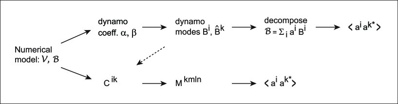
Figure 1: Survey of the computations reported in this paper. Starting point is the numerical dynamo model described in Section 2. The top line illustrates how the field ${\cal B}$ is decomposed in dynamo modes. First we obtain the dynamo coefficients, then the dynamo eigenmodes and their adjoints. End product are the correlation coefficients $\langle a^{i}a^{k*}\rangle$. This computational train is treated in Section 3. The correlation coefficients may also be computed theoretically, which requires an additional computation outlined in the bottom line and described in Section 4. Measured and theoretical correlation coefficients are compared in Section 5.2.

In Section 4 we recapitulate the theoretical mode excitation levels and in Section 5 we compare the numerical results with the theoretical predictions. Finally, in Section 6, we summarise and discuss our results.

2 Numerical model

We consider a Boussinesq fluid with electrical conductivity $\sigma$ in a rotating spherical shell $V$ and solve the momentum equation, the induction equation and a temperature equation as described in more detail by Olson et al. (1999). No-slip mechanical boundary conditions are applied and the magnetic field continues outside the fluid shell as a potential field. Convection is driven by a temperature difference $\Delta T$ between the inner and outer spherical boundaries. The equations are governed by four dimensionless parameters, these are the Ekman number $E=\nu/\Omega L^{2}$, the (modified) Rayleigh number $Ra=\alpha_{T}g_{0}\Delta TL/\nu\Omega$, the Prandtl number $Pr=\nu/\kappa$ and the magnetic Prandtl number $Pm=\nu/\eta$. Here, $\nu$ denotes the kinematic viscosity, $\Omega$ the angular rotation rate, $L$ the shell thickness, $\alpha_{T}$ the thermal expansion coefficient, $g_{0}$ the gravitational acceleration at the outer boundary, and $\kappa$ is the thermal and $\eta=1/\mu\sigma$ the magnetic diffusivity with the magnetic permeability $\mu$ and conductivity $\sigma$.

The model under consideration is taken from Olson et al. (1999) with $E=10^{-4}$, $Ra=334$, $Pm=2$ and $Pr=1$. The resulting convection pattern is strongly columnar and symmetric with respect to the equatorial plane, see Fig. 2. The magnetic field is largely dipolar, strictly antisymmetric with respect to the equatorial plane and approximately axisymmetric. The energy in the axisymmetric component of the field is about 40% of the total magnetic energy.

The magnetic energy density exceeds the kinetic energy density, as illustrated in Fig. 2. The magnetic Reynolds number $Rm=u_{\rm r.m.s.}L/\eta$ is approximately $88$. Here $u_{\rm r.m.s.}$ denotes the r.m.s. magnitude of the velocity. Although kinetic and magnetic energy densities vary chaotically in time, the dipole axis of the magnetic field is stable and reversals do not occur. This example belongs to the class of kinematically stable dynamos identified by Schrinner et al. (2010a), their model 2, which means that there exists no magnetic field that will grow exponentially if it is kinematically advanced with the time-dependent, saturated, velocity field taken from the self-consistent calculation.

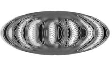
Figure 2: Top: The radial velocity ${\cal V}_{\rm r}$ in the corotating frame of the dynamo model under consideration. The snapshot has been taken at $r=0.62\,r_{0}$, where $r_{0}$ is the outer shell radius. The velocity component is normalised to its absolute maximum. Thus, the greyscale coding runs from $-1$, white, to $+1$, black, and the contour lines correspond to $\pm 0.1,\pm 0.3,\pm 0.5,\pm 0.7,\pm 0.9$. Bottom: Magnetic (upper curve) and kinetic energy densities of the model versus magnetic diffusion time $L^{2}/\eta$.

3 Mode decomposition

In principle the magnetic field of a dynamo may be decomposed in any suitable set of base functions. We could take, for example, the decay modes of a homogeneous sphere or spherical shell. However, there are reasons to prefer another set: the eigenfunctions of the dynamo operator averaged over time and azimuth of the numerical model, see Hoyng (2009) and Section 5. The dynamo operator describes the average dynamo action of a given flow. For statistically steady and kinematically stable dynamos, to which we restrict ourselves here, the actual magnetic field of the numerical model is expected to be well represented by the fundamental eigenmode and a few overtones. Since the magnetic field of the numerical dynamo model is largely axisymmetric, we restrict the decomposition to the axisymmetric dynamo modes. Likewise we ignore symmetric modes since the field of the model is strictly antisymmetric with respect to the equatorial plane.

A mode decomposition then requires three steps. The first is that we compute the dynamo coefficients $\alpha_{ij}$ and $\beta_{ijk}$ of the model. Then we determine the eigenfunctions and eigenvalues of the dynamo equation, and finally we decompose the field $\cal{B}$ of the numerical model in these eigenfunctions.

3.1 Properties and notations

Before we engage in details we summarise some of the notations and properties that we employ:

1. The magnetic field ${\cal B}$, vector potential ${\cal A}$, current ${\cal J}$ and the velocity ${\cal V}$ in the dynamo region $V$ are written in calligraphic font; ${\cal B}=\nabla\times{\cal A}$, etc. Furthermore, we make the usual split in mean flow $v$ and turbulent flow $u$: ${\cal V}=\mbox{\boldmath$v$}+\mbox{\boldmath$u$}$.

2. $B$ is the mean field $\langle{\cal B}\rangle$, and $\mbox{\boldmath$B$}^{i}$ are the eigenfunctions of the dynamo equation of the numerical model, briefly referred to as the dynamo modes. We use upper indices to enumerate modes and lower indices for vector components.

3. The mode decomposition makes use of the adjoint eigenfunctions, indicated by a hat $\ \hat{}\,$, e.g. $\,\hat{\!\mbox{\boldmath$B$}}{}^{k}$ is the adjoint of $\mbox{\boldmath$B$}^{k}$.

4. The adjoint operation and $\nabla$ commute. The basic entities are the field and its adjoint. The adjoint current $\,\hat{\!\mbox{\boldmath$J$}}{}^{k}$ is defined as $\nabla\times\,\hat{\!\mbox{\boldmath$B$}}{}^{k}$, likewise if $\,\hat{\!\mbox{\boldmath$B$}}{}=\nabla\times(\cdots)$, then $(\cdots)=\,\hat{\!\mbox{\boldmath$A$}}{}$.

5. We absorb the factor $4\pi/c$ in the definition of all currents. So ${\cal J}=\nabla\times{\cal B}$, $\,\,\hat{\!\mbox{\boldmath$J$}}{}^{k}=\nabla\times\,\hat{\!\mbox{\boldmath$B$}}{}^{k}$, etc.

6. $\mbox{\boldmath$b$}^{i}$ are the decay modes of the spherical shell $V$; the decay modes are self-adjoint, so we may adopt $\hat{\mbox{\boldmath$b$}}{}^{i}=\mbox{\boldmath$b$}^{i*}$; $\hat{\mbox{\boldmath$\jmath$}}{}^{i}=\mbox{\boldmath$j$}^{i*}=\nabla\times\mbox{\boldmath$b$}^{i*}$, and we shall assume that they are orthonormal:

   $$\int_{V+E}\mbox{\boldmath$b$}^{k*}\cdot\mbox{\boldmath$b$}^{i}\,{\rm d}^{3}\mbox{\boldmath$r$}\,=\,\delta^{ki}\ .$$ (1)

   Here $E$ is the vacuum exterior to $V$ (not to be confused with the Ekman number).

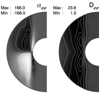
Figure 3: Two components of the dynamo coefficients. Left: $\alpha_{\varphi\varphi}$ in units of $\eta/L$. On the right: $D_{\varphi\varphi}=\eta+{\textstyle\frac{1}{2}}\beta_{\varphi r\theta}-{\textstyle\frac{1}{2}}\beta_{\varphi\theta r}$ in units of $\eta$. For each plot the grey scale is separately adjusted to its maximum modulus with white as negative and black as positive. The contour lines correspond to $\pm 0.1$, $\pm 0.3$, $\pm 0.5$, $\pm 0.7$, and $\pm 0.9$ of the maximum modulus.

3.2 Dynamo coefficients

The action of the small-scale turbulent flow $u$ on the mean magnetic field is parametrised by the so-called dynamo coefficients, $\alpha$ and $\beta$. They are, in general, tensors of second and third rank, respectively. The various coefficients describe, e.g., the anisotropic dynamo effects of helical flows ($\alpha$-effect), the transport of the mean magnetic field and the anisotropic turbulent magnetic diffusivity.

The dynamo coefficients are computed with the help of the test field method developed by Schrinner et al. (2005, 2007). For a set of suitably chosen test fields, the induction equation for the fluctuating field is solved with the actual flow of the numerical model, the electromotive forces are computed, and then averaged in azimuth and time. Finally the coefficients are derived from the projection of the mean electromotive forces on the corresponding test fields. For details we refer to Schrinner et al. (2007); Schrinner (2011). For axisymmetric mean fields the $\alpha$-tensor has 9 non-zero elements while the $\beta$-tensor has 18 non-zero entries. As an example we show in Fig. 3 two components for the dynamo model under consideration: $\alpha_{\varphi\varphi}$ and $D_{\varphi\varphi}=\eta+{\textstyle\frac{1}{2}}\beta_{\varphi r\theta}-{\textstyle\frac{1}{2}}\beta_{\varphi\theta r}$, i.e. the $\varphi\varphi$-component of the turbulent diffusivity plus the molecular diffusivity $\eta$. For more details on the representation of the dynamo coefficients we refer to Schrinner et al. (2007), in particular Eqs. (10)-(13) and (15e). The dynamo coefficients reflect the action of the convection columns on the mean magnetic field outside the inner core tangent cylinder. They are almost zero inside the tangent cylinder where no convection takes place.

Table 1: Eigenvalues of the first 13 antisymmetric and axisymmetric dynamo modes in units of $\eta/L^{2}$, numbered according to decreasing $\Re\lambda$, and computed as in Schrinner et al. (2010b), with $n_{\mathrm{max}}=16$, $l_{\mathrm{max}}=32.$ For a complex pair of modes, the larger mode number is taken to correspond to $\Im\lambda<0$.

mode number $i$	eigenvalue $\lambda_{i}$
$0$	$(-3.875,\ 0.00)$
$1,2$	$(-34.83,\ \pm 10.31)$
$3$	$(-40.63,\ 0.00)$
$4$	$(-42.88,\ 0.00)$
$5$	$(-70.13,\ 0.00)$
$6$	$(-72.25,\ 0.00)$
$7$	$(-76.44,\ 0.00)$
$8,9$	$(-98.22,\ \pm 43.87)$
$10$	$(-106.0,\ 0.00)$
$11$	$(-135.4,\ 0.00)$
$12,13$	$(-135.9,\ \pm 9.318)$

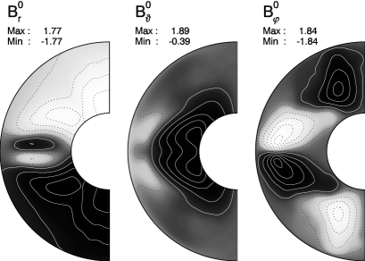
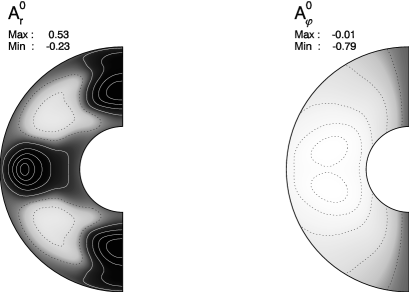
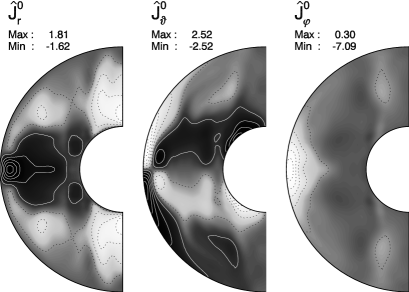
Figure 4: The magnetic field $\mbox{\boldmath$B$}^{0}$ (top), the vector potential $\mbox{\boldmath$A$}^{0}$ (middle), and the adjoint current $\,\hat{\!\mbox{\boldmath$J$}}{}^{0}$ (bottom) of the fundamental dipole mode of the numerical model. In the gauge we adopted for the vector potential (Schrinner et al., 2010b), $A^{0}_{\theta}$ is zero due to axisymmetry.

3.3 Dynamo modes

We next solve the eigenvalue problem of the dynamo equation

$$\lambda\mbox{\boldmath$B$}=\nabla\times D\mbox{\boldmath$B$}\ ,$$ (2)

with

$$D\mbox{\boldmath$B$}=\mbox{\boldmath$v$}\times\mbox{\boldmath$B$}+\mbox{\boldmath$\alpha$}\cdot\mbox{\boldmath$B$}-\mbox{\boldmath$\beta$}:(\nabla\mbox{\boldmath$B$})-\eta\nabla\times\mbox{\boldmath$B$}\ .$$ (3)

Here $v$ is the mean flow and $B$ the mean field. The eigenfunctions of the dynamo equation are denoted as $\mbox{\boldmath$B$}^{i}(\mbox{\boldmath$r$})$ and we refer to them as the ‘dynamo modes’. They are constructed by expanding them in the magnetic decay modes $\mbox{\boldmath$b$}^{\ell}(\mbox{\boldmath$r$})$ of the spherical shell $V$:

$$\mbox{\boldmath$B$}^{i}={\rm e}^{i\ell}\mbox{\boldmath$b$}^{\ell}$$ (4)

Summation convention over double upper indices is adopted. Expansion (4) is now inserted in Eq. (2), after which the eigenvalues $\lambda_{i}$ and the matrix elements ${\rm e}^{i\ell}$ may be determined as explained in Schrinner et al. (2010b). The computation of the matrix elements requires that the normalisation of $\mbox{\boldmath$B$}^{i}$ is fixed, and we suppose that that has been taken care of. Details are given in A. The advantage of the new method described by Schrinner et al. (2010b) is that the velocity and the dynamo coefficients do not have to be differentiated, as would be necessary in the traditional methods. This is important for the present study, as we obtain these coefficients and the velocity from the dynamo code in the form of numerical tables.

Since the dynamo modes $\mbox{\boldmath$B$}^{i}$ are in general not orthogonal we make use of the adjoint modes $\,\hat{\!\mbox{\boldmath$B$}}{}^{k}$. Together they form a biorthogonal set on $V+E$:

$$\int_{V+E}\,\hat{\!\mbox{\boldmath$B$}}{}^{k}\cdot\mbox{\boldmath$B$}^{i}\,{\rm d}^{3}\mbox{\boldmath$r$}\,=\,\int_{V}\,\hat{\!\mbox{\boldmath$J$}}{}^{k}\cdot\mbox{\boldmath$A$}^{i}\,{\rm d}^{3}\mbox{\boldmath$r$}\,=\,\delta^{ki}$$ (5)

The second relation follows by integrating by parts, and shows that currents and vector potentials also form a biorthogonal set on the volume $V$ of the dynamo. The adjoint modes may again be found with the help of an expansion in decay modes:

$$\,\hat{\!\mbox{\boldmath$B$}}{}^{k}={\rm f}^{ks*}\mbox{\boldmath$b$}^{s*}\ ,$$ (6)

and Schrinner et al. (2010b) show that ${\rm f}=({\rm e}^{-1})^{\dagger}$ where $\dagger$ indicates the Hermitean adjoint. For details and the question of gauge invariance we refer to this paper. Since the eigenmodes and their adjoints are constructed as linear combinations of the decay modes they automatically satisfy the boundary conditions, because the decay modes do so. We refer to Section 3.1 for a summary of the various magnetic field related concepts that we have introduced (model field $\cal{B}$, dynamo modes $\mbox{\boldmath$B$}^{i}$, decay modes $\mbox{\boldmath$b$}^{i}$, their adjoints, currents and vector potentials).

As explained above, we restrict the mode decomposition to antisymmetric and axisymmetric dynamo modes. The eigenvalues of the first of these modes are shown in Table 1. The fundamental mode $\mbox{\boldmath$B$}^{0}$ is non-periodic and antisymmetric with respect to the equator, and may, on that account, be representative for the geodynamo. Non-periodic modes $\mbox{\boldmath$B$}^{i}$ are themselves real. The structure of the fundamental mode $\mbox{\boldmath$B$}^{0}$ together with the corresponding vector potential $\mbox{\boldmath$A$}^{0}$ and adjoint current $\,\hat{\!\mbox{\boldmath$J$}}{}^{0}$ is shown in Fig. 4.

Remarkable is the large drop in growth rate beyond the fundamental mode which underlines the outstanding role of the fundamental mode in representing the magnetic field of this dynamo model. For completeness we mention that the spectrum of the symmetric modes is similar to that of the antisymmetric modes, but the fundamental symmetric mode decays more strongly, at a rate of $-6.298\,\eta/L^{2}$.

3.4 Field decomposition

The magnetic field ${\cal B}$ of the numerical dynamo model is represented by an expansion in dynamo eigenmodes $\mbox{\boldmath$B$}^{i}$:

$${\cal B}(\mbox{\boldmath$r$},t)=a^{i}(t)\mbox{\boldmath$B$}^{i}(\mbox{\boldmath$r$})$$ (7)

So we first construct the dynamo modes from the decay modes, and then we represent the field ${\cal B}$ of the dynamo as a superposition of dynamo modes. Because the dynamo modes (eigenfunctions of the dynamo equation) may be supposed to constitute a complete function set they may be used to represent any arbitrary magnetic field.

The expansion coefficients $a^{i}$ may be computed by taking the inner product with the adjoint $\,\hat{\!\mbox{\boldmath$B$}}{}^{k}$ and integrating over all space:

$$a^{k}\,=\,\int_{V+E}\,\hat{\!\mbox{\boldmath$B$}}{}^{k}\cdot{\cal B}\;{\rm d}^{3}\mbox{\boldmath$r$}\,=\,\int_{V}\,\hat{\!\mbox{\boldmath$J$}}{}^{k}\cdot{\cal A}\;{\rm d}^{3}\mbox{\boldmath$r$}\ .$$ (8)

Since $\mbox{\boldmath$B$}^{0}$ is real, the coefficient $a^{0}$ is real. To evaluate the integrals in (8) we compute first the adjoint currents $\,\hat{\!\mbox{\boldmath$J$}}{}^{k}={\rm f}^{k\ell*}\mbox{\boldmath$j$}^{\ell*}$ on the numerical grid, cf. Eq. (6). This needs to be done only once. Next we compute at each time step the vector potential ${\cal A}$. The integral $\smallint_{V}\,\hat{\!\mbox{\boldmath$J$}}{}^{k}\cdot{\cal A}\;{\rm d}^{3}\mbox{\boldmath$r$}$ in (8) follows by taking the inner product and summing over the grid. Because of the infinite volume and the power-law scaling of $\,\hat{\!\mbox{\boldmath$B$}}{}^{k}\cdot{\cal B}$ with radius, it is not a good idea to evaluate the other expression $\smallint_{V+E}\,\hat{\!\mbox{\boldmath$B$}}{}^{k}\cdot{\cal B}\;{\rm d}^{3}\mbox{\boldmath$r$}$. Fig. 5 shows $|a^{k}(t)|$ for $k=0$ and $k=1$ as a function of time, together with the averages $\langle|a^{k}|\rangle$ (horizontal lines). Once the expansion coefficients have been determined the computation of the cross correlation coefficient $\langle a^{k}a^{\ell*}\rangle$ is straightforward.

Two remarks on the magnitude of the expansion coefficients. The $a^{k}$ are of order unity, and that is a result of scaling: in the dynamo code $\cal{B}$ has been scaled to be of order unity. And the normalisation (18) makes that the integral in Eq. (8) is also of order unity, at least for the modes of lower order. The second remark is that by adopting the normalisation (18) we ensure that all dynamo modes, if excited alone and with the same amplitude (i.e. $a^{k}=1$ other $a^{i}=0$), have the same total magnetic energy, see A.

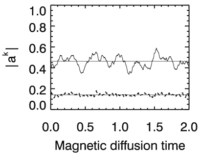
Figure 5: Modulus of the amplitude of the fundamental mode ($k=0$, top) and of the first overtone ($k=1$, broken line), as a function of time in units of the magnetic diffusion time $L^{2}/\eta$. The horizontal line indicates the mean modulus.

4 Theoretical mode excitation levels

The r.m.s. mode coefficients may be found from the evolution equation for the correlation coefficients derived in Hoyng (2009):

$$\left(\frac{{\rm d}}{{\rm d}t}-\lambda_{k}-\lambda_{\ell}^{*}\right)\langle a^{k}a^{\ell*}\rangle\,=$$

$$\qquad\qquad\qquad\left(M^{km\ell n}+M^{\ell nkm*}\right)\langle a^{m}a^{n*}\rangle\ .\qquad$$ (9)

(summation over $n,m$, not over $k,\ell$). The matrix elements $M^{km\ell n}$ are defined as integrals over velocity cross correlation functions:

$$M^{km\ell n}\,=\,\int_{0}^{\infty}\!{\rm d}\tau\,\langle C^{km}(t)C^{\ell n*}(t-\tau)\rangle\ .$$ (10)

The functions $C^{km}(t)$ are in turn averages of the turbulent flow $u$ over the volume of the dynamo weighted by ‘spatial filters’ defined by the dynamo modes:

$$C^{k\ell}(t)=-\int_{V}\;\mbox{\boldmath$u$}\cdot\,\hat{\!\mbox{\boldmath$J$}}{}^{k}\times\mbox{\boldmath$B$}^{\ell}\;{\rm d}^{3}\mbox{\boldmath$r$}\ .$$ (11)

This expression suggests that $C^{k\ell}$ may be interpreted as being proportional to the work done per unit time by a part of the Lorentz force on the flow $u$.

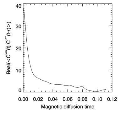
Figure 6: The cross correlation function $\langle C^{km}(t)C^{\ell n*}(t-\tau)\rangle$ as a function of the time shift $\tau$, for $k=\ell=1,\ m=n=0$. The vertical axis is in units of $(\nu/L^{2})^{2}=4(\eta/L^{2})^{2}$.

4.1 Computation of $M^{km\ell n}$

The turbulent flow $u$ must be measured and projected on a set of known vectors $\,\hat{\!\mbox{\boldmath$J$}}{}^{k}\times\mbox{\boldmath$B$}^{\ell}$, and summed over the spatial grid. This may be done on line after each new time step of the dynamo code. The result would be a set of time series $C^{k\ell}(t)$. However, the mean flow $v$ and therefore the turbulent flow $\mbox{\boldmath$u$}=\cal{V}-\mbox{\boldmath$v$}$ is not known until the end of the simulation, so we must adopt a more elaborate procedure. We project the full flow field $\cal{V}$ on $\,\hat{\!\mbox{\boldmath$J$}}{}^{k}\times\mbox{\boldmath$B$}^{\ell}$, and define $\tilde{C}^{km}$ as above but with the full flow field. The required cross correlation may now be computed from

$$\langle C^{km}(t)C^{\ell n*}(t-\tau)\rangle$$

$$\qquad\quad=\langle\tilde{C}^{km}(t)\tilde{C}^{\ell n*}(t-\tau)\rangle-\langle\tilde{C}^{km}\rangle\langle\tilde{C}^{\ell n*}\rangle\ .$$

(12)

A result is shown in Fig. 6. The computation of the averages $\langle\tilde{C}^{km}\rangle$ in (12) is straightforward, and we briefly explain how the cross correlation functions are computed, suppressing all details on the implementation in the dynamo code. Writing momentarily $x=\tilde{C}^{km}$ and $y=\tilde{C}^{\ell n*}$, we compute, for a given time $t$, an array of values $x(t)y(t-i\cdot\Delta\tau)$ for $i=0,..n$. Next we select other (later) starting times $t$, $N_{\rm av}$ in total, and average $x(t)y(t-i\cdot\Delta\tau)$ over these starting times $t$ for fixed $i$. In this way we obtain $\langle x(t)y(t-\tau)\rangle$ for time shifts $\tau$ ranging from 0 to $\tau_{\rm cu}=n\Delta\tau$. The upper limit $\tau_{\rm cu}$ to the various correlation times $\tau_{\rm c}$ is not known a priori but has to be determined empirically from graphs similar to Fig. 6. The results presented here have been derived with $\tau_{\rm cu}=0.113\,L^{2}/\eta$, $\Delta\tau=7.5\cdot 10^{-4}\,L^{2}/\eta$ and $N_{\rm av}=6\cdot 10^{4}$. Finally we determine $M^{km\ell n}$ by an integration over $\tau$, in accordance with Eq. (10), carried out in the post-processing.

5 Results

We shall now compare the numerical results with the theoretical predictions and draw some conclusions.

5.1 Applicability of the statistical theory

The statistical theory that we used here has been formulated by Hoyng (2009), and the conditions of the applicability of the theory have been worked out in Sections V and VI of that paper. The first requirement is that the correlation time $\tau_{\rm c}$ is short:

$$C^{k\ell}\tau_{\rm c}\ll 1\ .$$ (13)

In Hoyng (2009) $C^{k\ell}$ could be estimated only approximately, but here we can do better with the help of the numerical model. From Fig. 6 at $\tau=0$ we deduce that $C^{10}\simeq[38\cdot 4\,\allowbreak(\eta/L^{2})^{2}]^{1/2}\simeq 12\,\eta/L^{2}$. The correlation time may be taken as the $1/e$ time in Fig. 6: $\tau_{\rm c}\sim 0.01\,L^{2}/\eta$. In this way we obtain:

$$C^{10}\tau_{\rm c}\simeq 0.1\ .$$ (14)

$C^{k\ell}$ can be shown to increase slowly with mode number $k$ as $L/L_{k}$, where $L_{k}$ is the characteristic length scale in mode $k$ ($L_{k}<L_{0}=L$).

The second requirement is that the unperturbed evolution of the system is slow. Since the mean flow $v$ is very small, this condition reduces to the requirement derived in Hoyng (2009), relation (21):

$$\frac{\eta\tau_{\rm c}}{L_{k}L_{\ell}}\;\simeq\;0.01\;\frac{L^{2}}{L_{k}L_{\ell}}\;\ll\,1\ .$$ (15)

From these results we conclude that the first few dynamo modes of the numerical model obey the condition of a short correlation time and of a slow unperturbed evolution, though not by a wide margin. We return to this point in Section 5.2.

Figure 7: Mode excitation levels $\langle|a^{k}|^{2}\rangle$ as a function of the mode number defined in Table 1: $\ast=\langle|a^{k}|^{2}\rangle$ as measured from the numerical model; $\Diamond\ =\langle|a^{k}|^{2}\rangle$ computed from (16); $\triangle\ =\langle|a^{k}|^{2}\rangle$ computed from (9). The excitation levels have been normalised to that of the fundamental mode, whose value is measured to be $\langle|a^{0}|^{2}\rangle=0.226$. The levels of mode 1 and 2 are equal since they are a complex pair; likewise, the levels of mode 8 and 9 are equal.

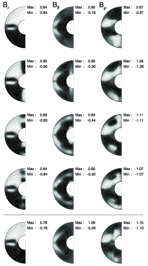
Figure 8: The bottom row shows the $r$, $\theta$ and $\varphi$ component of the dynamo field $\cal{B}$ averaged over azimuth and time. The rows above the horizontal line show the field expansion $\Sigma_{k=0}^{k=p}\;a^{k}\mbox{\boldmath$B$}^{k}$ averaged over the same period and truncated at various levels. At the top is $p=0$, in the downward direction followed by $p=5$, $p=7$ and $p=13$.

5.2 Mode excitation levels

We now come to the r.m.s. mode excitation levels. We consider first the special case that the fundamental mode is dominant, that is, $\langle|a^{0}|^{2}\rangle\ll\langle|a^{i}|^{2}\rangle$ for $i\geq 1$. In that case we may ignore all terms in the summation in the right hand side of Eq. (9) except $m=n=0$. We put ${\rm d}/{\rm d}t=0$ (the dynamo is supposed to be in a quasi-stationary state) and take $k=\ell$ to obtain:

$$\langle|a^{k}|^{2}\rangle\ \simeq\ \frac{\Re M^{k0k0}}{-\Re\lambda_{k}}\;\langle|a^{0}|^{2}\rangle\ .$$ (16)

Once the $M^{k0k0}$ have been computed as in Section 4.1, relation (16) allows us to obtain the overtone excitation levels relative to that of the fundamental mode. In much the same way we could also derive expressions for the cross correlations $\langle a^{m}a^{n*}\rangle$, but we restrict ourselves here to the autocorrelations. The result is plotted in Fig. 7 as $\Diamond$, while the measured overtone excitation levels are plotted as $\ast$. The agreement between theory and measurement seems reasonable to good for all modes except mode $5$, $8$ and $9$.

As it is not clear to what extent the fundamental mode amplitude is really dominant, we have investigated if the solution improves by employing the full equation (9). To this end we take again $k=\ell$ and ${\rm d}/{\rm d}t=0$ in Eq. (9) and evaluate the entire right hand side, the $M^{km\ell n}$ as in Section 4.1 and the $\langle a^{m}a^{n*}\rangle$ are measured from the numerical data. In the end we divide by $-2\Re\lambda_{k}$. The resulting excitation levels have been plotted as ${\triangle}$ in Fig. 7. Since the $\triangle$’s coincide closely with the $\Diamond$’s, our tentative conclusion is that the higher order terms in the summation in Eq. (9) may indeed be ignored, and that fundamental mode amplitude of the numerical model is in fact dominant.

The ‘flat level’ in Fig. 7 may be explained with the help of estimate (43) of Hoyng (2009):

$$\frac{\langle|a^{k}|^{2}\rangle}{\langle|a^{0}|^{2}\rangle}\,\sim\,N^{-1}\sim\,0.1\ ,$$ (17)

which agrees rather well with Fig. 7. Here $N$ is the number of convective elements, which we estimate to be of order 10 (Fig. 2). So while there is a good agreement at the qualitative level, we have no stringent explanation for the small measured excitation levels of modes $5$, $8$ and $9$. However, we recall that assumptions (14) and (15) are only marginally fulfilled, in particular for higher overtones. Moreover, we may have lost accuracy in each of the computational steps visualised in Fig. 1. Notably, the parametrisation of the electromotive force by the dynamo coefficients determined and thus the dynamo modes and their eigenvalues will be to some extent inaccurate (see also Schrinner et al., 2007; Schrinner, 2011).

It is tempting to interprete Fig. 7 as a spectrum, but the non-orthogonality of the dynamo modes renders such an interpretation impossible, see A for more details.

5.3 Representation of the field

The fundamental dynamo mode largely dominates the magnetic field as illustrated in Fig. 8. It is obvious that in particular the $r$ and $\theta$ components of the time and azimuthally averaged dynamo field $\cal{B}$ (bottom row) are fairly well represented by the fundamental dynamo mode alone (top row). The $\varphi$ component improves somewhat by including a few overtones, but as we do so the $r$ and $\theta$ components deteriorate slightly. This problem is fixed again by including a few more modes. By the time we have incorporated some $10$ modes the agreement is quite good.

The behaviour of the $\varphi$ component shows a peculiarity inherent to an expansion in non-orthogonal modes: the approximation is not monotonous. Another illustration is the fact that mode 6 and 7 have a large amplitude, see Fig. 7, but they almost cancel each other in the field expansion (7), and together they contribute little to the representation of the field, as can be seen in the middle row of Fig. 8.

6 Discussion and summary

Dipolar geodynamo models in the low Rossby number regime are governed by one fundamental dynamo mode. On average, the fundamental mode has zero growth rate, whereas more spatially structured overtones are highly diffusive. Small-scale contributions to the magnetic field (i.e. overtones) result from the deformation of the fundamental mode by the turbulent flow; subsequently, they decay due to Ohmic diffusion. The ratio between both processes determines their excitation levels. This intuitive picture proposed and formalised by Hoyng (2009) is confirmed by the satisfactory agreement between theoretically predicted and numerically measured excitation levels in Fig. 7. Moreover, from a methodological point of view, the consistency of the whole ‘train’ of computational steps illustrated in Fig. 1 is confirmed.

As noted by Schrinner et al. (2010a), the dominance of the fundamental mode in models of this dynamo regime is closely related to their time dependence and to the saturation of the magnetic field. The dipole field in these models is stable and polarity reversals are inhibited, because the damping of the magnetic field results in the preference of always the same fundamental mode, which is continuously quenched and rebuilt. As a by-product, these models may be treated kinematically (see Schrinner et al., 2010a) and the mode analysis presented in this study is applicable. However, a generalisation of our approach to models beyond the kinamatically stable regime would require to place velocity modes and magnetic field modes on equal footing (Courvoisier et al., 2010; Rheinhardt and Brandenburg, 2010) and is therefore not easily feasible.

We expand the magnetic field in dynamo modes which are eigenfunctions of a non-selfadjoint operator. They form a complete function set but are in general not orthogonal. This has severe consequences for the interpretation of Fig. 5 or Fig. 7; they cannot be interpreted as spectra. In general, there is no correspondence between the modulus of a mode coefficient and the contribution of its associated mode to the dynamo field $\cal{B}$. Modes with a comparatively large amplitude may in fact contribute only very little. This has been demonstrated in Fig. 8 for modes 6 and 7 and is the reason for the non-monotonous series approximation (7). The ambiguity of mode coefficients is a general problem inherent to most of the attempts to model dynamo action by amplitude equations. It could be avoided by expanding $\cal{B}$ in a orthogonal function set, e.g. the decay modes, instead of the dynamo modes. On the other hand, dynamo modes lead to a rather accurate representation of $\cal{B}$ with a minimum number of modes taken into account. Furthermore, the compact formulas obtained for the excitation levels, (9) and (16), require that $\cal{B}$ is expanded in eigenfunctions of the dynamo operator (Hoyng, 2009). In short, an expansion in dynamo modes has been preferred because it leads to the simplest description and allows for theoretical predictions.

In this study, we have applied the mode analysis developed by Hoyng (2009) to a geodynamo model in the low Rossby number regime. We find satisfactory agreement between theoretical predictions and numerical simulations. The expansion of $\cal{B}$ in dynamo modes may serve as a useful analytical tool to interpret numerical dynamo models. Besides direct numerical simulations, low-order models have been successful in illustrating the possible interaction of large-scale modes of different symmetries in planetary cores (e.g. Pétrélis et al., 2009; Gissinger, 2010). The work presented here connects both approaches and allows for the possibility to compare predictions from low-order models with direct numerical simulations.

Appendix A Mode normalisation and spectral interpretation

First of all, we note that relation (5) does not fix the normalisation of the dynamo modes: given a biorthogonal set $\,\hat{\!\mbox{\boldmath$B$}}{}^{k},\mbox{\boldmath$B$}^{i}$ we may construct others, viz.: $\mbox{\boldmath$B$}^{k}\rightarrow\mu\mbox{\boldmath$B$}^{k}\ ,\quad\,\hat{\!\mbox{\boldmath$B$}}{}^{k}\rightarrow(1/\mu)\,\hat{\!\mbox{\boldmath$B$}}{}^{k}$, where the factor $\mu$ may depend on the mode number $k$. These new sets also obey relation (5). We choose to remove the remaining ambiguity, up to an overall phase factor $\exp({\rm i}\phi)$, by imposing that

$$\int_{V+E}\mbox{\boldmath$B$}^{k*}\cdot\mbox{\boldmath$B$}^{k}\,{\rm d}^{3}\mbox{\boldmath$r$}\,=\,\int_{V}\mbox{\boldmath$J$}^{k*}\cdot\mbox{\boldmath$A$}^{k}\,{\rm d}^{3}\mbox{\boldmath$r$}\,=\,1\$$ (18)

(no summation over $k$). The middle relation follows as usual by integrating by parts. An immediate consequence of this normalisation is that

$$({\rm e}{\rm e}^{\dagger})^{kk}=1\ ,$$ (19)

(no summation over $k$). The diagonal elements of ${\rm e}{\rm e}^{\dagger}$ are all unity. To see this insert relation (4) in eq. (18) and use the orthogonality of the decay modes.

The normalisation (18) makes sense for two reasons. The first is that in the special case of self-adjoint modes we may choose $\,\hat{\!\mbox{\boldmath$B$}}{}^{k}=\mbox{\boldmath$B$}^{k*}$, and then relation (18) follows automatically from (5). The second reason is that, loosely speaking, dynamo modes with the same amplitude $a^{k}$ but excited alone, contain the same total magnetic energy. We shall now make this statement precise.

The energy density of the magnetic field may be written as
$\mathcal{B}\cdot\mathcal{B}=a^{i}a^{k*}\mbox{\boldmath$B$}^{i}\cdot\mbox{\boldmath$B$}^{k*}$, according to Eq. (7). Next, we insert twice relation (4), integrate over all space, and use the orthogonality of the decay modes. Finally we apply relation (19). The result is:

$$\int_{V+E}\mathcal{B}\cdot\mathcal{B}\,{\rm d}^{3}\mbox{\boldmath$r$}\,=\,\sum_{k}\,|a^{k}|^{2}\,+\,\sum_{i\neq k}\;({\rm e}{\rm e}^{\dagger})^{ik}\,a^{i}a^{k*}\,.$$

(20)

This expression shows that if only one mode is excited at unit amplitude, $a^{j}=1$ and all other $a^{k}$ zero, then the total magnetic energy $\smallint_{V+E}\,\mathcal{B}\cdot\mathcal{B}\,{\rm d}^{3}\mbox{\boldmath$r$}$ is also unity, independent of the mode number $j$.

Now if the dynamo modes were self-adjoint, then Eq. (5) becomes $\smallint_{V+E}\mbox{\boldmath$B$}^{k*}\cdot\mbox{\boldmath$B$}^{i}\,{\rm d}^{3}\mbox{\boldmath$r$}\,=\,\delta^{ki}$. Upon inserting again relation (4) we get ${\rm e}{\rm e}^{\dagger}={\rm I}$, i.e. the matrix ${\rm e}$ is now unitary. In that case the second term in (20) drops out, and we are left with $\smallint_{V+E}\,\mathcal{B}\cdot\mathcal{B}\,{\rm d}^{3}\mbox{\boldmath$r$}=\sum_{k}\,|a^{k}|^{2}$. And that leads straight away to a spectral interpretation of Fig. 7, because the mode number scale on the horizontal axis can be converted into a wave number scale. But in general we are stuck with Eq. (20) as a whole, and contributions to the magnetic energy remain stored in the nonzero mode overlaps $\smallint_{V+E}\mbox{\boldmath$B$}^{k*}\cdot\mbox{\boldmath$B$}^{i}\,{\rm d}^{3}\mbox{\boldmath$r$}$.

References

- Aubert et al. (2008) Aubert, J., Aurnou, J., Wicht, J., 2008. The magnetic structure of convection-driven numerical dynamos. Geophys. J. Int. 172, 945–956.
- Busse (1975) Busse, F.H., 1975. A model of the geodynamo. Geophys. J. Roy. Astron. Soc. 42, 437–459.
- Christensen and Aubert (2006) Christensen, U.R., Aubert, J., 2006. Scaling properties of convection-driven dynamos in rotating spherical shells and application to planetary magnetic field. Geophys. J. Int. 166, 97–114.
- Christensen and Wicht (2007) Christensen, U.R., Wicht, J., 2007. Numerical dynamo simulations. In Treatise of Geophysics, Volume 8: Core Dynamics, Ed. G. Schubert (Amsterdam: Elsevier), 245-282.
- Christensen et al. (2010) Christensen, U.R., Aubert, J., Hulot, G., 2010. Conditions for Earth-like geodynamo models. Phys. Earth Planet. Inter. 296, 487–496.
- Courvoisier et al. (2010) Courvoisier, A., Hughes, D.W., Proctor, M.R.E., 2010. Self-consistent mean-field MHD. Proc. Roy. Soc. Lond. 466, 583–601.
- Dormy et al. (1998) Dormy, E., Cardin, P., Jault, D., 1998. MHD flow in a slightly differentially rotating spherical shell, with conducting inner core, in a dipolar magnetic field. Earth Planet. Sci. Lett. 160, 15–30.
- Driscoll and Olson (2009) Driscoll, P., Olson, P., 2009. Effects of buoyancy and rotation on the polarity reversal frequency of gravitationally driven numerical dynamos. Geophys. J. Int. 178, 1337–1350.
- Gissinger (2010) Gissinger, C., 2010. Dipole-quadrupole dynamics during magnetic field reversals. Phys. Rev. E 82, 056302.
- Glatzmaier and Roberts (1995) Glatzmaier, G.A., Roberts, P.H., 1995. A three-dimensional self-consistent computer simulation of a geomagnetic field reversal. Nature 337, 203–209.
- Glatzmaier and Coe (2007) Glatzmaier, G.A., Coe, R.S., 2007. Magnetic polarity reversals in the core. In Treatise of Geophysics, Volume 8: Core Dynamics, Ed. G. Schubert (Amsterdam: Elsevier), 283–298.
- Hoyng (2009) Hoyng, P., 2009. Statistical dynamo theory: mode excitation. Phys. Rev. E 79, 046320.
- Kageyama and Sato (1997) Kageyama, A., Sato, T., 1997. Generation mechanism of a dipole field by a magnetohydrodynamic dynamo. Phys. Rev. E 55, 4617–4626.
- Kuang and Bloxham (1997) Kuang, W., Bloxham, J., 1997. An Earth-like numerical dynamo model. Nature 389, 371–374.
- Kutzner and Christensen (2002) Kutzner, C., Christensen, U.R., 2002. From stable dipolar towards reversing numerical dynamos. Phys. Earth Planet. Inter. 131, 29–45.
- Olson et al. (1999) Olson, P., Christensen, U., Glatzmaier, G.A., 1999. Numerical modeling of the geodynamo: Mechanisms of field generation and equilibration. J. Geophys. Res. 104, 10383–10404.
- Pétrélis et al. (2009) Pétrélis, F., Fauve, S., Dormy, E.,Valet, J.-P., 2009. Simple mechanism for reversals of Earth’s magnetic field. Phys. Rev. Lett. 102, 144503.
- Rheinhardt and Brandenburg (2010) Rheinhardt, M., Brandenburg, A., 2010. Test-field method for mean-field coefficients with MHD background. Astron. Astrophys. 520, A28.
- Roberts and Glatzmaier (2000) Roberts, P.H., Glatzmaier, G.A., 2000. Geodynamo theory and simulations. Rev. Mod. Phys. 72, 1081–1123.
- Sarson and Jones (1999) Sarson, G.R., Jones, C.A., 1999. A convection driven geodynamo reversal model. Phys. Earth Planet. Inter. 111, 3–20.
- Schrinner (2011) Schrinner, M., 2011. Global dynamo models from direct numerical simulations and their mean-field counterparts; in preparation.
- Schrinner et al. (2005) Schrinner, M., Rädler, K.-H., Schmitt, D., Rheinhardt, M., Christensen, U.R., 2005. Mean-field view on rotating magnetoconvection and a geodynamo model. Astron. Nachr. 326, 245–249.
- Schrinner et al. (2007) Schrinner, M., Rädler, K.-H., Schmitt, D., Rheinhardt, M., Christensen, U.R., 2007. Mean-field concept and direct numerical simulations of rotating magnetoconvection and the geodynamo. Geophys. Astrophys. Fluid Dynamics 101, 81–116.
- Schrinner et al. (2010a) Schrinner, M., Schmitt, D., Cameron, R., Hoyng, P., 2010a. Saturation and time dependence of geodynamo models. Geophys. J. Int. 182, 675–681.
- Schrinner et al. (2010b) Schrinner, M., Schmitt, D., Jiang, J., Hoyng, P., 2010b. An efficient method for computing the eigenfunctions of the dynamo equation. Astron. Astrophys. 519, A80.