Galactic cold cores II. Herschel study of the extended dust emission around the first Planck detections

Abstract

Context. Within the project $Galactic$ $Cold$ $Cores$ we are carrying out Herschel photometric observations of cold interstellar clouds detected with the Planck satellite. The three fields observed as part of the Herschel science demonstration phase (SDP) provided the first glimpse into the nature of these sources. The aim of the project is to derive the physical properties of the full cold core population revealed by Planck.

Aims. We examine the properties of the dust emission within the three fields observed during the SDP. We determine the dust sub-millimetre opacity, look for signs of spatial variations in the dust spectral index, and estimate how the apparent variations of the parameters could be affected by different sources of uncertainty.

Methods. We use the Herschel observations where the zero point of the surface brightness scale is set with the help of the Planck satellite data. We derive the colour temperature and column density maps of the regions and determine the dust opacity by a comparison with extinction measurements. By simultaneously fitting the colour temperature and the dust spectral index values we look for spatial variations in the apparent dust properties. With a simple radiative transfer model we estimate to what extent these can be explained by line-of-sight temperature variations, without changes in the dust grain properties.

Results. The analysis of the dust emission reveals cold and dense clouds that coincide with the Planck sources and confirm those detections. The derived dust opacity varies in the range $\kappa(250\,\mu{\rm m})\sim$ 0.05–0.2 cm² g^-1, higher values being observed preferentially in regions of high column density. The average dust spectral index $\beta$ is $\sim$1.9–2.2. There are indications that $\beta$ increases towards the coldest regions. The spectral index decreases strongly near internal heating sources but, according to radiative transfer models, this can be explained by the line-of-sight temperature variations without a change in the dust properties.

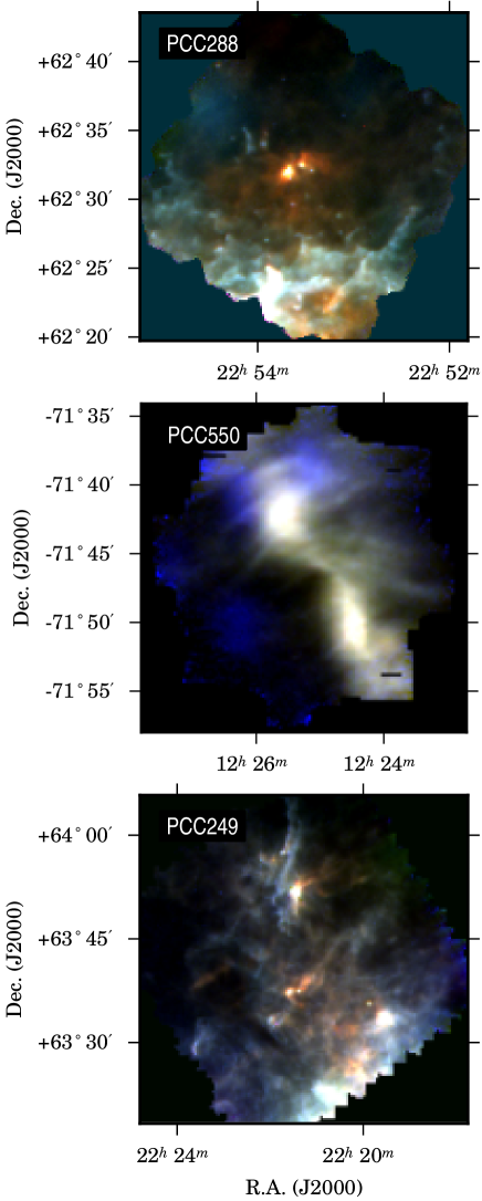
Figure 1: Three-colour figures of the three SDP fields. The red, green, and blue colours correspond to the 250 $\mu$m, 160 $\mu$m, and 100 $\mu$m intensities (PCC288 and PCC249) or the 350 $\mu$m, 250 $\mu$m, and 160 $\mu$m intensities (PCC550). Only the area covered by both the PACS and SPIRE instruments is shown. See Appendix A for images of the individual bands.

1 Introduction

A major question in star formation studies is how the main features of the process depend on the initial conditions in cold molecular clouds. The masses of the formed stars, the star formation efficiency, the differences between clustered and isolated star formation, and the timescales are all closely linked to the properties of dense cloud cores. In order to understand these dependencies, we need to study a large sample of molecular clouds and the pre-stellar cores within them. The molecular lines are a central tool in the study of molecular clouds. However, in the cloud cores many molecules have frozen onto dust grains making it difficult to carry out quantitative analysis with molecular line data alone (e.g., Kramer et al. Kramer1999 (1999)). One has to resort to observations of the dust component of the clouds, either using the extinction or the dust emission as a tracer of the mass distribution.

The recently launched Herschel and Planck satellites represent a significant step forward in sub-millimeter studies by eliminating the atmospheric effects from observations. The satellites enable sensitive measurements of the dust emission in Galactic interstellar clouds, Planck over the whole sky and Herschel in smaller regions but with higher angular resolution. The satellites provide the complementarity needed for a study of a full cross section of the Galactic cold core population. Because of its high sensitivity and the coverage of the sub-millimetre wavelengths dominated by cold dust emission, the Planck all-sky maps provide an unbiased census of cold dust clouds and, in particular, of compact pre-stellar cloud cores. The survey of cold compact dust clouds is one of the goals in the Galactic science programme of Planck. In the Herschel Open Time Key Programme Galactic Cold Cores, we use the Herschel PACS and SPIRE instruments to map about one hundred target fields that are selected on the basis of the Planck survey. This study was begun during the Herschel Science Demonstration Phase (SDP) when three fields were observed.

Table 1: The observed fields

Target	RA (J2000)	DEC (J2000)	Map size (PACS/SPIRE)
PCC 249	22 21 17.6	+63 42 25	50$\arcmin$/50$\arcmin$
PCC 288	22 53 31.3	+62 31 44	18$\arcmin$/30$\arcmin$
PCC 550	12 25 16.5	$-$71 46 03	18$\arcmin$/30$\arcmin$

The main features of the compact sources found in the SDP fields were reported in Juvela et al. (Juvela2010 (2010)). In this paper we concentrate on the dust emission at large scales. We are interested in the cloud properties, their temperature and column density distributions. However, we also want to study the dust component itself. These are not unrelated questions because the derived cloud masses depend on the assumptions of the dust opacity and spectral index. Conversely, the variations in dust properties should be related to the physical conditions within the clouds.

The dust spectral index and its temperature dependence have received much attention because they provide additional information on the chemical composition, structure, and the size distribution of interstellar dust grains (e.g., Ossenkopf & Henning ossenkopf1994 (1994); Krugel & Siebenmorgen Krugel1994 (1994); Mennella et al. Mennella1998 (1998); Boudet et al. Boudet2005 (2005); Mény et al. Meny2007 (2007); Compiègne et al. Compiegne2011 (2011)). The observations consistently show an inverse $T-\beta$ relation (e.g., Dupac et al. Dupac2003 (2003), Hill et al. Hill2006 (2006), Veneziani et al. Veneziani2010 (2010) and the initial Herschel results including Anderson et al. Anderson2010 (2010) and Rodon et al. Rodon2010 (2010)). However, the reliability of this relation is notoriously difficult to estimate because any noise present in the measurements produces a similar anticorrelation (Schwartz et al. Schwartz1982 (1982), Dupac et al. Dupac2003 (2003), Shetty et al. 2009a ). Shetty et al. (2009b ) studied the importance of observational noise and temperature variations on the reliability of the derived dust properties. In the presence of line-of-sight temperature variations, the observed dust spectral index $\beta$ will underestimate the real spectral index of the dust grains. The estimated colour temperatures are not only biased towards the warm regions but, for example in the two component models of Shetty et al. (2009b ), could be even higher than any of the real dust temperatures. Similar results were obtained by Malinen et al. (Malinen2011 (2011)) who studied synthetic observations produced by combining MHD modelling and radiative transfer calculations. They concluded that the presence of protostellar radiation sources can further increase the bias in the observed $\beta$ values and can produce an apparent inverse $\beta$–$T$ relation that is difficult to separate from any intrinsic relation the dust grains may have. Malinen et al. (Malinen2011 (2011)) also noted that when the spectral index varies over the wavelength range included in the spectral energy density (SED) fit, the derived spectral index can rise even above the real $\beta(\lambda)$ of the dust anywhere in that interval. Because an error in the spectral index is always associated with a compensating error in the temperature, this affects the mass estimates and could even bias the derived density profiles of compact objects.

Like the spectral index, also the absolute value of the dust absorption cross section, $\kappa$, is expected to be variable. This could be caused by a change in the abundance of different dust populations, a change in the grain size distribution (see, e.g., Steinacker et al. Steinacker2010 (2010)), or a change in the composition of individual grains. For the sub-millimetre observations, the effects should again be strongest in dense and cold regions where the grains acquire ice mantles and may more easily coagulate to form larger grains with $\kappa$ values up to 3–4 times higher (e.g., Ossenkopf & Henning ossenkopf1994 (1994), Krugel & Siebenmorgen Krugel1994 (1994), Stepnik et al. Stepnik2003 (2003)). An error in $\kappa$ automatically translates to a similar fractional error in the mass estimates. The absolute value of $\kappa$ is not easy to measure because it requires an independent column density estimate that is equally or more reliable over the $A_{\rm V}$ range for which sub-millimetre observations exist.

In this paper we study these questions with the help of photometric Herschel observations. We start by deriving the colour temperature (Sect. 3.1) and column density (Sect 3.2) maps of the three SDP fields. This first analysis is done with a constant value of the spectral index $\beta$. In Sect. 3.3 we proceed to study the evidence for variations in the dust spectral index. With simultaneous fits of colour temperature and $\beta$, we calculate maps of the apparent spectral index paying special attention to the error sources that could affect the obtained values or the morphology of the $\beta$ maps. By comparing the results with the near-infrared reddening of background stars, we calculate maps of dust sub-millimetre opacity (Sect. 3.4). To complement this analysis, we present in Sect. 4 a simple radiative transfer model for the field PCC288 and use the results to estimate the difference between the apparent $\beta$ and the real spectral index of the dust grains. After a discussion in Sect. 5 we present our final conclusions in Sect. 6.

2 Observations

The Planck satellite is performing all sky surveys at nine wavelengths between 350 $\mu$m and 1 cm (Tauber et al. Tauber2010 (2010)). With the detection methods described in Montier et al. (Montier2010 (2010)), three target fields were selected from the Planck First Light Survey (see Table 1) for photometric observations with the Herschel PACS and SPIRE instruments (for details about Herschel, see Pilbratt et al. Pilbratt2010 (2010), Poglitsch et al. Poglitsch2010 (2010), and Griffin et al. Griffin2010 (2010)). The Herschel observations were performed in November and December 2009. The field PCC249 was observed in the parallel mode and the fields PCC288 and PCC550 in the normal scan mapping, one instrument at a time (see Juvela et al. Juvela2010 (2010)). The fields are shown in Fig. 1. The data were reduced with the Herschel Interactive Processing Environment (HIPE) v.2. The PACS maps were created using the madmap algorithm. The processing includes some high pass filtering. In order to minimize the removal of large scale structure, the length of the filter window was kept equal to the scan length. The SPIRE maps are the product of direct projection onto the sky and averaging of the time ordered data.

Table 2: The uncertainties of the map zero levels

Target	Wavelength	Zero level uncertainty
	($\mu$m)	MJy sr-1
PCC 288	100	14.3
	160	10.3
	250	3.1
	350	1.2
	500	0.4
PCC 550	100	0.81
	160	1.41
	250	0.43
	350	0.23
	500	0.08
PCC 249	100	4.4
	160	2.6
	250	2.9
	350	0.7
	500	0.21
1Zero level calculated using map averages.

In order to study dust properties over the whole fields we need to establish a zero point for the intensity scales. We use the Planck maps (data release DX4, available within the Planck core teams) at 350 $\mu$m and 550 $\mu$m and the Improved Reprocessing of the IRAS Survey (IRIS, Miville-Deschenes & Lagache MAMD2005 (2005)) maps at 100 $\mu$m. The highest frequency Planck channels have been calibrated with FIRAS (Piat et al. 2002) and the IRIS data have been calibrated according to DIRBE. When necessary, we interpolate these reference data for the Herschel bands using a modified black body curve $B_{\nu}\nu^{2}$ fitted to the nearest two wavelength points.

The 100 $\mu$m band contains a contribution from very small grains (VSG). The effect is approximately similar in the IRIS and PACS 100 $\mu$m bands and does not affect the calibration comparison at that wavelength. However, the presence of VSG at 100 $\mu$m could bias the values interpolated to 160 $\mu$m and 250 $\mu$m. Therefore, before the interpolation, we subtract from the IRIS 100 $\mu$m data the VSG contribution estimated with the Désert et al. (Desert1990 (1990)) dust model. The radiation field is scaled so that the model reproduces the observed temperature of the big grains (BG) that dominate the emission wavelengths longer than 100 $\mu$m. The predicted ratio of VSG and BG emission at 100 $\mu$m is used to correct the IRIS data. Because the ratio depends on the estimated BG temperature, the correction has to be done iteratively. Finally, we do a least squares fit to Herschel surface brightness (convolved to a resolution of 4.3$\arcmin$) vs. Planck/IRIS and use the offset to set the zero level of the Herschel maps while keeping the original gain calibration. For the PCC550 PACS observations the fits remained uncertain because of the small amount of surface brightness variation. In this case the zero point was estimated using the difference in the average surface brightness rather than the extrapolation to zero Planck/IRIS surface brightness.

In the comparison between Planck and IRIS, the data should be colour corrected because this could affect the quality of the least squares fit. The colour corrections were calculated for modified black body spectra $B_{\nu}(T)\nu^{2}$ that were fitted to the observations after a preliminary estimation of the zero points. All observations, including Planck and IRIS data, were colour corrected before repeating the least squares fits. The corrections can be applied consistently only if the offsets of the Herschel and Planck/IRIS maps are already correct and therefore also this correction needs to be done iteratively. However, the colour corrections are less than 10%, and a sufficient accuracy is reached already on the second iteration. The subsequent analysis was carried out using these colour corrected observations.

The statistical uncertainties of the offsets were estimated with the bootstrap method and are listed in Table 2. The uncertainties are of the order of 1 MJy sr^-1 but smaller at the longest wavelengths with the lowest surface brightness. The error estimates are larger for the PACS channels apart from the field PCC550 where, as explained above, the quoted offsets are calculated using average surface brightness values.

3 Observational results

In this section we present the colour temperature, column density, and spectral index maps. The relation between these and the intrinsic dust properties is discussed in the later sections.

3.1 Colour temperature maps

The colour temperature maps of the large grain emission were estimated using the 100 $\mu$m, 160 $\mu$m, 250 $\mu$m, 350 $\mu$m, and 500 $\mu$m observations. The colour temperatures were first calculated with a constant value of the spectral index, $\beta=2.0$. The validity of this approximation is investigated in Sect. 3.3. The use of a constant $\beta$ can be justified even when the assumption is not strictly true because it enables more robust estimation of one colour temperature that characterizes the fields. As discussed in Sect. 4, the colour temperature is often an imprecise tracer of the physical dust temperatures.

All data were smoothed to the resolution of the SPIRE 500 $\mu$m map (37$\arcsec$) using a Gaussian kernel. As discussed in Sect. 2, the determination of the zero points of the surface brightness scales and the correction for the VSG contribution were done iteratively together with the calculation of the colour temperatures. In the fit the relative weight of the data are set assuming 10% uncertainty for the SPIRE and 20% for the PACS measurements. The temperature maps are shown in Fig. 2.

Figure 2: Dust colour temperature maps for the three SDP fields. The calculations assume a fixed value of the spectral index, $\beta=2.0$. The map resolution is $\sim$37$\arcsec$ and the contours are drawn one Kelvin apart.

3.2 Column density maps

The column densities were calculated using the modified blackbody fits that resulted in the colour temperature maps of Fig. 2. Like the spectral index, the dust absorption cross section may vary from region to region but the analysis was performed using a constant value of $\kappa_{850}$=0.02 cm² g^-1 (see Juvela et al. Juvela2010 (2010)). With a $\nu^{2}$ dependence this corresponds to $\kappa_{250}$=0.23 cm² g^-1. The column density maps are presented in Fig. 3 where we also show 9 arcmin diameter circles around the positions of the Planck detections. These were used in Juvela et al. (Juvela2010 (2010)) to estimate the masses of the regions.

The column densities were transformed into mass with the distances adopted by Juvela et al. (Juvela2010 (2010)), 800 pc, 225 pc, and 800 pc for PCC288, PCC550, and PCC249, respectively. In the same order, the total masses of the areas displayed in Fig. 3 are $\sim$890 $M_{\sun}$, $\sim$31 $M_{\sun}$, and $\sim$3800 $M_{\sun}$. The masses above the given column density contours, and inside the 9 arcmin apertures, are listed in Table 3. The statistical errors are small and the mass uncertainty is dominated by the uncertainties of the calibration ($\sim$10%), the dust opacity (up to a factor of two), and the cloud distance (typically $\sim$30% corresponding to a $\sim$50% uncertainty in the mass.

3.3 Dust spectral index

The 100 $\mu$m–500 $\mu$m data were also fitted with modified blackbody curves $B_{\nu}(T)\nu^{\beta}$ keeping both the colour temperature $T$ and the spectral index $\beta$ as free parameters. We masked out the borders of the maps ($\sim 3\arcmin$) and the northern end of the field PCC288 where the column density map and the map of dust opacity (see Sect. 3.4 and Sect. 5.3) show a suspicious feature. The colour temperature and spectral index maps are shown in Fig. 4 and representative SEDs in Fig. 5. The median values of $\beta$ are 2.21, 2.21, and 1.86 for PCC288, PCC550, and PCC249, respectively. The same fits without the 100 $\mu$m data are shown in Appendix B.2.

Figure 3: Maps of the hydrogen column density $N({\rm H})$ derived with the colour temperature maps of Fig. 2. The maps have a resolution of $\sim$37$\arcsec$ and the contours are drawn at levels where $log_{\rm 10}N(H)$ equals 21.5, 21.8, and 22.1. The circles show the 9 arcmin apertures used in Juvela et al. (Juvela2010 (2010)).

Table 3: The mass estimates of the observed fields or parts of the fields that are defined by a column density limit or correspond to 9 arcmin apertures (regions $P$, $P1$, and $P2$).

Field	Region	Mass ($M_{\sun}$)
PCC 288	full field	1108
	$log_{\rm 10}N>21.8$	785
	$log_{\rm 10}N>22.1$	242
	$P$	288
PCC 550	full field	36.2
	$log_{\rm 10}N>21.8$	13.9
	$P1$	12.2
	$P2$	11.3
PCC 249	full field	3802
	$log_{\rm 10}N>21.8$	1763
	$log_{\rm 10}N>22.1$	627
	$P1$	252
	$P2$	259

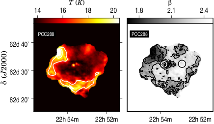
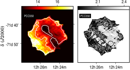
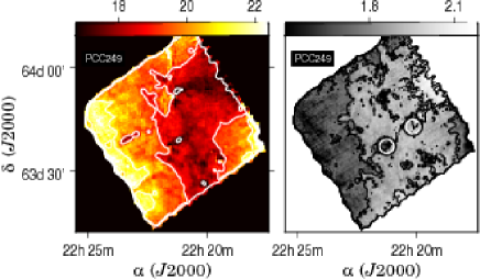
Figure 4: The colour temperature and dust spectral index maps. The values have been determined by a fit to the observations between 100 $\mu$m and 500 $\mu$m. The circles indicate the positions for which the spectra are shown in Fig. 5.

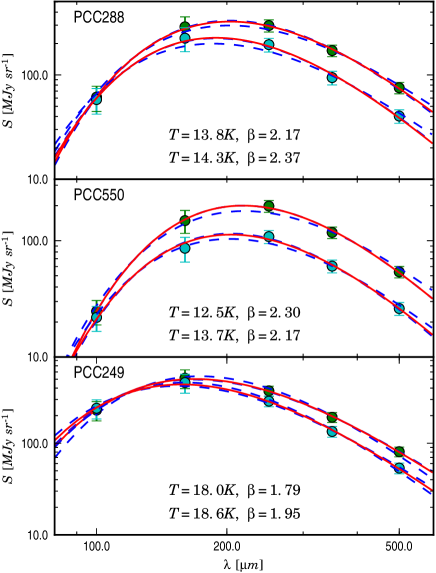
Figure 5: Spectral energy distributions for selected positions. The measurements correspond to a single pixel at the centre of the circles shown in Fig. 4 (after convolution to the resolution of the 500 $\mu$m observations). The temperature and the spectral index are quoted in the frames, the first values corresponding to the upper SED curve. The dashed lines are the fits with a constant spectral index value of $\beta=1.7$ or $\beta=2.3$.

In Fig. 6 we show the relations between the derived spectral indices and the colour temperatures. For three randomly selected pixels, the black contours show where the $\chi^{2}$ value of the SED fit has doubled from its minimum value.

To get the first idea of the possible effect of the calibration uncertainty, we compared two cases where we add errors to the 250 $\mu$m and the 500 $\mu$m maps and recalculate the colour temperature and spectral index maps. The wavelengths were chosen because their relative intensities are important in determining the spectral index. The map offsets were first changed by the values listed in Table 2 and the surface brightness values were scaled corresponding to a 10% gain uncertainty. The changes at the two wavelengths were made in opposite directions in order to have the maximum effect in the derived $\beta$ values. By applying the $\sim$1$\sigma$ shifts both in the gain and in the offset and at both wavelengths simultaneously, we should get a conservative estimate of the uncertainties. In Fig. 6, the resulting shifts of the observed ($T,\beta$) pairs are shown for the three random pixels. The full maps of the maximum and minimum $\beta$ values are shown in the Appendix, Sect. B.1.

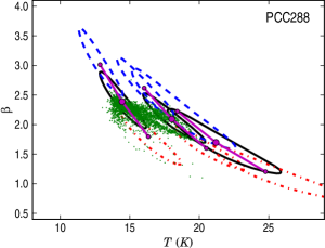
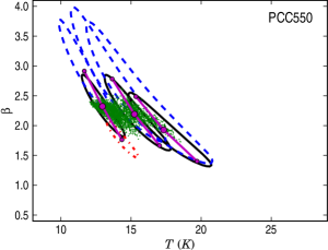
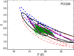
Figure 6: The observed temperature dependence of the spectral index in the three fields. The values are shown for individual pixels (green dots). For three selected pixels, the black contours show the limit at which the $\chi^{2}$ value of the SED fit has doubled from its minimum value. For the same pixels the smaller symbols (joined with solid lines) show the extreme values allowed by the calibration uncertainty (see text). The error regions for these extreme cases are drawn with dashed and dash-dot lines.

3.4 Dust opacity

We calculated extinction maps at a 1.5$\arcmin$ resolution using stars from the Two Micron All Sky Survey (2MASS, Skrutskie et al. Skrutskie2006 (2006)) and the NICER method (Lombardi & Alves Lombardi2001 (2001)). The values of $A_{\rm V}$ are obtained from NIR colour excess assuming an extinction law with $R_{\rm V}$=3.1. The zero level of the extinction was set with the Schlegel et al. (Schlegel1998 (1998)) extinction map. The extinction estimates enable us to estimate the sub-millimetre dust opacity relative to the visual extinction. The extinction is converted to total ISM mass with the Bohlin et al. (Bohlin78 (1978)) relation, $N({\rm HI+H_{2}})\sim 1.87\times 10^{21}\,A_{\rm V}$ that is multiplied by 1.4 $m_{\rm H}$ to account for the mass of helium. The conversion is done for easier comparison with the literature but the conversion factor itself is appropriate mainly for diffuse medium and may vary across the fields.

Figure 7 shows the 250 $\mu$m opacity maps derived from the SED fits done with $\beta=2.0$. The median values in the fields PCC288, PCC550, and PCC249 are 0.11, 0.064, and 0.061 cm² g^-1. The opacities obtained with fixed value of $\beta=2.0$ and the free $\beta$ are identical to within 20%. In the central part of PCC288 the values rise close to $\kappa(250\,\mu{\rm m})\sim$0.22 while in the northern colder region of PCC249 (corresponding to the Planck detection P1) the peak value is even higher, above $\sim 0.3$ cm² g^-1. The value used for the mass estimates in Sect. 3.2 was 0.23 cm² g^-1. This is clearly above the median values but roughly consistent with the values associated with the highest column densities. However, in the field PCC550 the values remain everywhere below $\kappa(250\,\mu{\rm m})=$ 0.12 cm² g^-1. Our typical opacity of 0.1 cm² g^-1 corresponds to $\tau$(250$\mu$m)=2.3$\times 10^{-25}$/H, slightly more than twice the value found in diffuse medium (Boulanger et al. Boulanger1996 (1996)).

4 Radiative transfer model of PCC288

To find out the level at which temperature variations along the line-of-sight may bias the observed values of the spectral index and the dust temperature, we made a simple model of the PCC288 region. The model was not intended as a fit to the PCC288 observations but is only used to estimate the general observational biases in a setting similar to this field. The model was based on the column density map shown in Fig. 3 and represents a box with a size of 5.4 pc (for $d$=800 pc). The line-of-sight density profile was gaussian with a FWHM that was 0.4 pc towards the densest part of the cloud and increased up to 1.6 pc in regions of low column density. The numbers roughly correspond to the scales of the central clump and the whole field but are basically ad hoc values. In particular, the density distribution of the model is quite smooth with a maximum density of only 3.7$\times 10^{4}$ cm^-3. Because also the wavelength dependence of the spectral index could bias the observed $\beta$ values (see Malinen et al. Malinen2011 (2011)), the modelling was done with a modified version of the normal Milky Way dust model (Draine Draine2003 (2003)) where $\beta$ was set to a constant value of 2.0 for all wavelengths $\lambda>100\mu$m. The cloud is illuminated from the outside by an isotropic interstellar radiation field (ISRF; Mathis Mathis83 (1983)). Three blackbody radiation sources with a temperature of 2000 K and luminosities of 10, 20, and 50 $L_{\sun}$ were added to represent internal heating. We show the results for a model where the column densities and the strength of the ISRF were scaled so that the surface brightness levels match the observations of PCC288 to $\sim 30\%$.

Because the proper handling of regions near the internal sources requires high spatial resolution, the model was sampled onto a hierarchical grid with the smallest cell size corresponding to the resolution of 1024³ uniform grid. The dust temperature distributions were solved with a radiative transfer program that is based on our Monte Carlo code (Juvela & Padoan Juvela2003 (2003)) but has been adapted for use with hierarchical grids (Lunttila et al., in preparation). The obtained surface brightness maps at 160 $\mu$m, 250 $\mu$m, 350 $\mu$m, and 500 $\mu$m were analysed to derive colour temperature and spectral index maps. Noise was not added to the synthetic observations and all wavelengths were given equal weight in the ($T$, $\beta$) fitting. The results are shown in Fig. 8 where the three internal sources are clearly visible (in order of increasing luminosity from West to East). The left hand frame shows the difference between the observed colour temperature and the mass weighted average of the true temperature. In the region shown, the dust temperature is overestimated by between $\sim$0.25 K in the most diffuse areas and $\sim$8 K at the position of the strongest source. The median error is $\sim$0.8 K. An error in the temperature is associated with an opposite change in the spectral index. In a fit with a fixed value of $\beta=2$, the median error would be only 0.4 K. At a temperature of $T=15$ K, this would correspond to a less than 15% underestimation of column density. If $\beta$ is kept as a free parameter, the 0.8 K bias leads to a $\sim$30% error in column density when the estimate is based on $\kappa$ at $160\,\mu{\rm m}$. This decreases to only $\sim$10% when the estimate is based on 500 $\mu{\rm m}$. However, close to the sources the errors remain large, at least a factor of two.

In Fig. 8, the median value of the observed spectral index is $\beta$=1.92 which is only slightly smaller than the actual value of the dust model, $\beta$=2.0. The values are more biased in areas of high column density and the observed $\beta$ is consistently below 1.9 in the south. At the position of the sources $\beta$ is reduced further to a minimum value of 1.56. The observations provide good estimates of the spectral index only in the more diffuse regions but also at a certain distance from the sources where the internal heating apparently helps to keep the temperature constant along the line-of-sight. Although the column density is highest in the central clump, the bias is higher in the south, further away from the heating sources.

Figure 7: Maps of the dust opacity derived from the comparison of the NIR extinction maps and SED fits with a fixed value of the spectral index, $\beta=2.0$. The values are given for 250$\mu$m and relative to the total ISM mass. The contours are drawn starting with the value of 0.05 cm² g^-1 and with a step of 0.02 cm² g^-1 (PCC550) or 0.03 cm² g^-1 (PCC288 and PCC249).

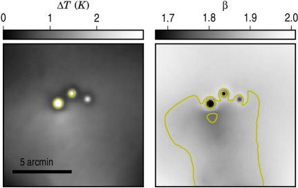
Figure 8: Results of the radiative transfer model of the PCC288 region. The left hand frame shows the difference between the colour temperature derived from synthetic observations and the real mass averaged dust temperature in the model. The right hand frame shows the obtained spectral index $\beta$. The contours are drawn at $\Delta T=1\,$K and $\Delta T=2\,$K and at $\beta$=1.8 and $\beta=$1.9.

5 Discussion

5.1 Colour temperatures

The calculation of the colour temperature maps for the full Herschel fields confirmed the Planck detections of cold dust emission. Even in the field PCC249, with active star formation and a high average colour temperature, the Planck detections correspond to regions where the colour temperatures, $T\sim 15$ K, are $\sim$2 degrees below the values of the surrounding areas. The Planck detections are based on the cold dust signature that remains when the warm component traced by the 100 $\mu$m IRIS maps has been subtracted (Montier et al. Montier2010 (2010)). This does not require a low colour temperature for the total emission. The separation of the warm and the possible cold component is more uncertain in warm regions where the warm component is strong and must be subtracted with higher relative accuracy. The PCC249 sources are very bright with peak surface brightness reaching in both PACS and the 250 $\mu$m SPIRE band several thousand MJy sr^-1. The Planck observations were able to locate the two nearby cold regions despite the fact that, according to Herschel, they are small and thus beam diluted: the Planck beams have a significant contribution also from the warmer surrounding regions.

In the analysis performed with a fixed spectral index value of $\beta=2.0$, the minimum colour temperatures were 13.8 K, 13.1 K, 15.6 K, and 14.8 K for PCC288, PCC550, and the northern and the southern areas in PCC249, respectively. These are a couple of degrees higher than the values reported in Juvela et al. (Juvela2010 (2010)) where temperatures were calculated after the subtraction of the local background. In spite of the different nature of the fields, the minimum temperatures are rather similar. Of course, even the background subtracted observations do not give a true picture of the coldest temperatures that inside the cores are likely to be below 10 K (e.g., Crapsi et al. Crapsi2007 (2007); Harju et al. Harju2008 (2008)). With radiative transfer modelling of the dust continuum observations one could derive an upper limit for the central temperature but once the temperature is reduced close to 6 K, the cold dust will be difficult to detect even with Herschel observations. In our simple model of the field PCC288, the minimum physical dust temperature was only $\sim$2 K lower than the minimum colour temperature. It is very likely that in the real clumps the central densities rise higher than in our radiative transfer model and therefore also reach lower physical temperatures.

5.2 Cloud masses and dust opacity

In Juvela et al. (Juvela2010 (2010)) the masses were estimated only for compact objects, with a fixed circular aperture and with background subtraction. The masses were quoted also for a 9 arcmin diameter aperture and these can now be compared with the values of Table 3 that were obtained without background subtraction. In PCC288, the estimate has increased by a factor of two from 140 $M_{\sun}$ to 288 $M_{\sun}$. In the case of PCC550 the background level is small and the change is much smaller. The previous values of 9.2 $M_{\sun}$ and 8.1 $M_{\sun}$ for P1 and P2, respectively, have been replaced by 12.2 $M_{\sun}$ and 11.3 $M_{\sun}$. In PCC249 the intensity levels are again high and also the contrast between the emission in the selected apertures and the surrounding reference areas is small. As a result, the masses obtained without background subtraction are much larger. The previous estimates of 90 $M_{\sun}$ (area $P1$) and 93 $M_{\sun}$ (area $P2$) have increased to 252 $M_{\sun}$ and 259 $M_{\sun}$. Differences are, of course, not surprising because the new measurements are for the whole mass along the line-of-sight while the old ones correspond to the column density excess within the aperture.

In PCC249, the new values are in better agreement with mass estimates from molecular line observations. Wang et al. (Wang2009 (2009)) obtained from ¹³CO(2 –1) observations a value of 1700 $M_{\sun}$ for a region that corresponds to our area $P1$. The estimate was calculated for a cloud distance of 1.67 kpc which, with the distance of $d=800$ pc assumed here, translates to $\sim$390 $M_{\sun}$. The value derived from Herschel data is still lower but already $\sim$65% of this number. On the other hand, the situation has not changed much for PCC550 where the masses obtained from molecular line studies (Vilas-Boas et al. VilasBoas1994 (1994); see Juvela et al. Juvela2010 (2010)) are also higher than our values. In PCC550-P2 the molecular line data gave a mass of 16.5 $M_{\sun}$ and the $\sim$50% discrepancy is still not very serious. However, for the core P1 (core Mu5 in Vilas-Boas et al. VilasBoas1994 (1994)) the CO analysis lead to a value of $\sim 33$ $M_{\sun}$ that is three times our estimate. The uncertainty of $\kappa$ can explain most of this discrepancy. The values derived in Sect. 3.4 were all below $\kappa(250\,\mu{\rm m})=0.15$ cm² g^-1 with a median value of 0.073 cm² g^-1. With $\kappa(250\,\mu{\rm m})=0.085$ cm² g^-1 the mass estimate of P1 would be in perfect agreement with the value obtained from the line observations. The radiative transfer model of PCC288 hinted that the column density estimates may be biased. In the case of PCC550 the final answer to this question may be provided by the detailed radiative transfer modelling that is currently under way (Ysard et al., in preparation). One can also question the accuracy of the CO mass estimates. The fractional abundances are not accurately known, the observations of the cold regions may be affected by some degree of molecular depletion (e.g., PCC550), and, conversely, the optical depths of the employed ¹³CO lines can become high enough so that radiative transfer effects can bias the results (e.g., self-absorption affecting the observed ¹³CO/C¹⁸O line ratios). Considering all the sources of uncertainty, the mass estimates obtained from the lines and from dust continuum are in good agreement.

The median values of the dust absorption cross sections $\kappa(250\mu{\rm m})$ obtained from the comparison with NIR extinction are 0.13, 0.073, and 0.055 cm² g^-1 for the fields PCC288, PCC550, and PCC249, respectively. The peak values are higher by more than a factor of two and, in PCC550 and PCC249, are associated with regions of higher column density. This behaviour is expected and could be explained by an increase in grain sizes. In PCC288, there is some indication that the dust opacity has increased in the central clump, close to the column density maximum. The increase towards the North corner is very likely only an artifact. The results could change noticeably even within the limits set by the accuracy of the zero points of the surface brightness scale. Nevertheless, the results suggest spatial variations at least by a factor of two. Most of our $\kappa(250\,mu{\rm m})$ values are in the range 0.05–0.2 cm² g^-1. Scaled with $\nu^{2}$, this corresponds to $\kappa(850\,\mu{\rm m})$=0.004–0.017 cm² g^-1. The $A_{\rm V}$ values were calculated assuming an extinction law with $R_{\rm V}$=3.1. This is appropriate for most areas but not necessarily for the densest cores. By adopting $R_{\rm V}$=5.5, the extinction values would decrease by $\sim$16%. Taking into account a possible decrease in the ratio $N(H)/A_{\rm V}$ the calculated dust opacities could increase further by more than 30% (see Evans et al. Evans2009 (2009), Draine Draine2003 (2003), and the online tables). This would further strengthen the case for an increasing sub-millimetre dust opacity in the cold and dense cores.

The opacities can be compared with values found in other studies. Using COBE measurements, Boulanger et al. (Boulanger1996 (1996)) derived an effective dust cross section for high latitude diffuse medium. At 850 $\mu$m, the obtained values are $\kappa(850\,\mu{\rm m})$=0.005 cm² g^-1 in agreement with the low end of our measurements. In the dark cloud IC 5146, Kramer et al. (Kramer2003 (2003)) found the values to vary from $\kappa_{850}/\kappa_{V}\sim 1.3\times 10^{-5}$ in warm regions (20-30 K) to $\sim 5\times 10^{-5}$ in colder regions with $T\sim 12$ K. With the conversion used in Sect. 3.4, these correspond to $\sim$0.003 cm² g^-1 and 0.011 cm² g^-1, in general agreement with our range of values. However, there are also dense and cold clouds where similar increase of dust opacity has not been observed. Nutter et al. (Nutter2008 (2008)) reported observations of a filament in Taurus and concluded that these can be modelled accurately without any spatial variations of dust properties. Juvela et al. (Juvela2009 (2009)) estimated for a Corona Australis molecular cloud filament a $\kappa$ value that was almost consistent with values found in diffuse clouds. This in spite of the fact that the region had more than 20^m of visual extinction and had a minimum colour temperature of $\sim$11 K although, on the other hand, the sub-millimetre measurements may have suffered from some spatial filtering. The results should be tested, possibly with the help of Herschel observations, to confirm whether the dust behaviour is this different in apparently similar clouds or whether the results could be explained by the difficulty of reaching an accuracy of measurements that is needed for a reliable determination of dust opacities.

5.3 Spectral indices

We fitted the observed ($T$, $\beta$) values of Fig. 4 with two analytical formulas, $\beta=A(T/20{\rm K)}^{-\alpha}$ and $\beta=(\delta+\omega T)^{-1}$. The parameters of the relations are listed in Table 4. The obtained $T(\beta)$ relations are steeper than reported in Dupac et al. (Dupac2003 (2003)) who fitted PRONAOS observations using the latter formula. Our relation is closer to the results from the Archeops experiment (Désert et al. Desert2008 (2008)) where the observations fit a relation $\beta=AT^{-\alpha}$ with an exponent value of $\alpha=0.66\pm 0.054$. The error estimates in Table 4 do not reflect the true uncertainty but only the accuracy of the curve fitting. One source of uncertainty is the accuracy to which the very small grain contribution could be subtracted from the 100 $\mu$m data. However, the temperature and spectral index maps derived without the 100 $\mu$m band are relatively similar to the results shown in Fig. 4 (see Appendix B.2). We will next examine the reliability of the detection of the spectral index variations in the presence of other error sources.

Calibration errors affect the ($T$, $\beta$) values mostly in a systematic fashion. In Fig. 6, we indicated for three representative pixels the shifts that would result from a 10% change in the gain calibration combined with a change in the offset that is equal to the uncertainties listed in Table 2. The calibration errors tend to move all points along a trajectory similar to that caused by random noise without much affecting the detection of an inverse $T-\beta$ relation. In the field PCC550, the spectral index reaches values $\beta\sim$2.35 at the locations of the two cores. In the high-$\beta$ version (calibration errors causing higher 250 $\mu$m and lower 500 $\mu$m surface brightness) the centre of the PCC550 filament would reach $\beta\sim 2.7$ while the background would remain at $\beta\sim$2.4. Opposite changes in the calibration would decrease the spectral index values in the filament to a value $\sim$2, still 0.2–0.3 units above the background. This shows that the increase of dust opacity within the PCC550 filament is robust against calibration errors although the uncertainty in the absolute value of $\beta$ is high, close to $\sim$0.4. The effects of a different calibration are similar in the other two fields, changing the absolute level of $\beta$ without a clear change in the morphology.

We used Monte Carlo simulations to quantify the noise bias and the evidence for a negative $\beta-T$ correlation. We added noise to the surface brightness measurement and repeated the fit of the $\beta(T)=AT^{-\alpha}$ relation.The statistical uncertainty of the surface brightness measurements, $\sigma_{\rm S}$, was estimated from the difference between the observed maps and the SED fits with a free $\beta$ parameter. These are conservative estimates because the residuals are affected also by calibration errors. The calibration uncertainty $\sigma_{\rm C}$ was assumed to consist of a 10% uncertainty in the gain calibration and the zero point uncertainties listed in Table 2. To see how sensitive the extracted values are on the statistical noise alone, we carried out one set of simulations where $\sigma_{\rm S}$ was added to the observed maps. However, we mainly compare the original observations with reference simulations with a flat $\beta(T)$ relation. These are based on the SED fits that were made with $\beta=2.0$. In the first set of simulations $\sigma_{\rm S}$ and $\sigma_{\rm C}$ were added to the input maps. In the second set of simulations one quarter of each surface brightness map was additionally scaled with a random factor corresponding to a 10% relative error. This simulates mapping artifacts, $\sigma_{\rm M}$, whose effect is fundamentally different from both $\sigma_{\rm S}$ (affecting each pixel independently) and $\sigma_{\rm C}$ (affecting all pixels simultaneously). While $\sigma_{\rm C}$ can shift all the ($T$, $\beta$) points along almost a fixed trajectory, without a noticeable change in the best fitting $\beta(T)$ relation, the mapping artifacts will increase the dispersion of the ($T$, $\beta$) values along the noise-induced $\beta(T)$ curve. This could be misinterpreted as a stronger evidence of an inverse relation between $\beta$ and $T$. The comparison between the SED fits and the surface brightness maps suggested the presence of some such artifacts (see Appendix B). In PCC249, these were below $\sim$5% apart from the northern end of the 160 $\mu$m map where, within an area less than 5% of the whole map, the residual rises between 10% and 20%. In PCC288 the artifacts remain below 10% when the northern corner has been masked out. The same applies to PCC550 except for the 160 $\mu$m map where the difference to the SED fit is above 10% over about one third of the map and reaches values 20–30% over an area less than 10% of the full map. By introducing a 10% error in the quarter of the mapped area and in all the frequency bands, we are certain to obtain a conservative estimate of the mapping artifacts, especially in PCC288 and PCC249.

Figure 9 shows the distribution of the parameters $\alpha$ in this Monte Carlo study, each resulting from the simulation of 500 sets of synthetic surface brightness maps. For each set of frequency maps, the colour temperatures and the spectral indices were estimated pixel by pixel, and the analytical $\beta(T)$ formulas were fitted to the results. The distribution $S1$ corresponds to the observed maps with added noise, $\sigma_{\rm S}$. The distributions $R1$ and $R2$ correspond to simulations with a constant value of $\beta=2$, $R1$ containing $\sigma_{\rm S}$ and $\sigma_{\rm C}$ and $R2$ additionally the mapping errors $\sigma_{\rm M}$. The vertical lines show the parameter values obtained directly from the observations.

Because of the noise-induced anticorrelation between $T$ and $\beta$, the $\alpha$ values are positive even when the input data correspond to a constant value of $\beta=2.0$. For the same reason, the distributions $S1$ are shifted relative to the observed values and are narrow only because the effect is almost identical in all Monte Carlo realizations. In the fields PCC288 and PCC249, the observed $\alpha$ values are higher than most values in the $R1$ distribution. If mapping artifacts can be ignored, this indicates a real anticorrelation between temperature and the observed spectral index. The hypothesis $\alpha>0$ gets probabilities 97% and 99% in the case of PCC288 and PCC249, respectively. However, with the simulated mapping artifacts the reference distributions $R2$ is much wider and the corresponding probabilities are reduced to 69% and 66%. The detections are no longer statistically significant but the numbers depend critically on the actual level of $\sigma_{\rm M}$. We believe that the noise values used in the simulation were conservative and the truth lies somewhere between the cases $R1$ and $R2$. Therefore, the Monte Carlo study gives some, although weak evidence for a non-flat $\beta(T)$ relation. In the case of PCC550, the values of $\alpha$ were higher in the simulations than in observations. This is possible if the mapping artifacts conspired to produce a low $\alpha$ value or may indicate overestimation of the errors.

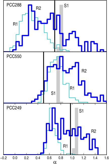
Figure 9: Results of the Monte Carlo study where the distribution of the values ($T$, $\beta$) is modelled with a function $\beta(T)=AT^{-\alpha}$. The vertical lines show the values of the parameter $\alpha$ estimated from the observations. The histograms $S1$ shows the distribution of the $\alpha$ values for observations with the added noise $\sigma_{\rm S}$. These are compared to simulations with $\beta=$2.0 containing the noise components $\sigma_{\rm S}$ and $\sigma_{\rm C}$ (distribution $R1$) or with additional simulated mapping artifacts, $\sigma_{\rm M}$ ($R2$, see the text for details).

Table 4: Parameters of the $\beta(T)$ fits.

	$\beta(T)=A(T/20{\rm K})^{-\alpha}$		$\beta(T)=(\delta+\omega T)^{-1}$
Target	$A$	$\alpha$	$\delta$	$\omega$
PCC 288	1.89(0.02)	0.62(0.03)	0.18(0.02)	0.018(0.001)
PCC 550	1.90(0.02)	0.44(0.02)	0.26(0.02)	0.014(0.001)
PCC 249	1.77(0.01)	0.97(0.02)	0.02(0.01)	0.027(0.001)

The Monte Carlo study showed that the global analysis of ($T$, $\beta$) points does not give a conclusive proof of spectral index variations. That analysis is not sensitive to very localized $\beta$ variations while it may be significantly affected by artifacts that are more likely to exist close to map edges and far from our dense sources. In Fig. 4, many of the spectral index variations are clearly correlated with actual cloud structures and, therefore, are unlikely to be caused by mapping artifacts. In PCC288 the spectral index increases from $\sim$2.2 at the boundaries to $\sim$2.5 in the central clump before decreasing to $\sim$1.5 at the location of the strongest warm source at the centre of the map. In PCC249 the warm sources are similarly associated with spectral index minima, $\beta\sim$1.0 near PCC249-P1 and $\sim$1.3 near PCC249-P2, while the values in the central map otherwise are between 1.8 and 2.2. It is clear that warm sources are associated with significantly lower $\beta$. The evidence for high $\beta$ values ($>>$2) towards the coldest clumps is somewhat weaker because it comes from larger scales that might be affected by mapping artifacts. However, in PCC288 and PCC550, $T$ and $\beta$ are clearly anticorrelated also in the regions with $T<$15 K. In PCC249 the situation is similar at large scales but not in the cores PCC249-P1 and PCC249-P2. These are very near to strong radiation sources which may have affected the spectral index estimates.

We conclude that there is strong evidence of spatial variations in the apparent dust spectral index and the magnitude of these changes is likely to be at least $\Delta\sim 0.2$ and can be up to $\Delta\sim 1$ towards warm, internally heated sources. The simple model of the PCC288 field showed that these apparent variations do not necessarily indicate an equal change in the dust properties. In the model, the spectral index of the grains could be 0.2–0.3 units higher than what is observed (Sect. 4). This applies to regions of high column density and without internal heating. The effect is opposite to the observed correlation between the column density and $\beta$ and further supports the idea of higher $\beta$ values for the dust grains in the cold cores. This behaviour is expected on the basis of laboratory measurements and can be explained by the properties of the grain materials at low temperature (Mennella et al. Mennella1998 (1998); Boudet et al. Boudet2005 (2005); Mény et al. Meny2007 (2007)). On the other hand, the low values of $\beta$ that were observed towards the warm sources in PCC288 can be fully explained by line-of-sight temperature variations. It will be difficult to determine whether also the intrinsic spectral index of the grains is lower in such regions (see also Malinen et al., Malinen2011 (2011)).

The exact relation between the observed and real $\beta$ depends on the properties of the object in question (density structure, strength of the external radiation field, nature of the internal sources etc.) and the results of our radiative transfer model cannot be generalized very far. We have started detailed modelling of the observations of PCC550. The results of that study will give us a better idea on how the observed spectral index variations, if real, are related to the actual dust properties. This may also shed new light on the reliability of the mass estimates derived from Herschel observations (Ysard et al., in preparation).

The possible presence of mapping artifacts was found to be the main problem in the evaluation of the observational $T$–$\beta$ relation. In new observations larger map sizes and increased redundancy would help to reduce such artifacts and make it easier to evaluate their impact. The situation may be improved with better data reduction methods and, in the future, one could also use Planck data to check for low resolution artifacts in the long wavelength Herschel data. When combined with far-infrared data, the Planck observations themselves are very suitable for the study of the spectral index variations and will be used to examine the situation also in cold cores and clumps (Planck Collaboration 2011a , 2011b ).

6 Conclusions

We have studied Herschel surface brightness measurements of three areas where the Planck satellite data indicated the presence of significant amounts of cold dust. By analysing surface brightness maps at wavelengths between 100 $\mu$m and 500 $\mu$m we map the dust colour temperature, dust opacity, and dust spectral index variations over the fields. The results lead to the following conclusions:

• The colour temperature maps confirm the Planck detections of cold dust. The analysis of the total intensity leads to minimum colour temperature of 13–15 K in the three fields.

• The results show an increase in the dust opacity towards colder and denser cloud regions. The range of values for the dust absorption cross section was estimated to be $\kappa(250\,\mu{\rm m})\sim$ 0.05–0.2 cm² g^-1, in agreement with previous studies.

• The median values of the observed spectral indices were between 1.9 and 2.2. We witnessed an inverse relation between the colour temperature and the spectral index. A Monte Carlo study indicated but did not conclusively prove a temperature dependence of $\beta$ beyond what could be produced by observational errors. However, because the changes are well correlated with column density, we believe the variations to be real. Very low values down to $\beta\sim$1.0 were observed towards warm sources but these are likely to be caused mainly by temperature variations rather than changes in the grain characteristics.

• With the help of a simple radiative transfer model, we examined the relation between the observed and intrinsic spectral indices. The results show that the intrinsic $\beta$ value of the dust grains is underestimated in regions of high column density and, therefore, the observations may also underestimate the real variation of the spectral index. On the other hand, the flat spectrum near internal heating sources can be explained by the line-of-sight temperature variations without any change in the dust properties.

Appendix A Frequency maps

Figures 10–12 show the 100 $\mu$m, 160 $\mu$m, 250 $\mu$m, and 350 $\mu$m surface brightness maps for the three SDP fields. The maps for 500 $\mu$m are not included but their appearance, apart from the lower intensity and lower spatial resolution, is almost identical with the 350 $\mu$m maps.

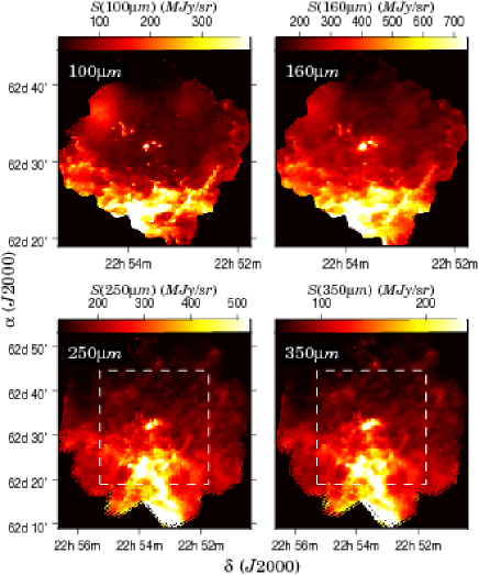
Figure 10: Surface brightness maps of the field PCC288. The zero point of the intensity scale has been set by comparison with the IRIS and Planck maps. In the lower frames the dashed line corresponds to the size of the upper frames showing the PACS observations.

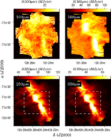
Figure 11: Surface brightness maps of the field PCC550.

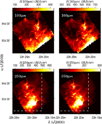
Figure 12: Surface brightness maps of the field PCC249.

Appendix B Residual maps at 160 $\mu$m–500 $\mu$m

The quality of the $B_{\nu}(T)\nu^{\beta}$ fits and the maps themselves can be evaluated by examining the residual maps at the five wavelengths used in the SED fit. These maps are shown in Figs. 13–15.

In PCC288 the average residuals are $-4.0$, 16.9, 6.7, $-6.3$, and 1.4 MJy sr^-1 in the five bands in the order of increasing wavelength. The corresponding values are $-$0.35, 2.4, 2.4, $-1.9$, and 0.4 MJy sr^-1 in the field PCC550 and $-3.8$, 17.3, $-0.7$, $-1.6$, and 0.47 MJy sr^-1 in the field PCC249. Allowing some errors in the gain, the estimated accuracies of the offsets (see Table 2) appear to have been realistic.

In PCC288 the largest residuals, $\sim 100$ MJy sr^-1, are found at the centre of the 160 $\mu$m map. This is associated with the brightest point source and is still less than 10% of the surface brightness. In Fig. 15 the residual images are strongly saturated and one can see both negative and positive values on the two sides of a source. Although the residuals reach several hundred MJy sr^-1 these are only at a $\sim$5% level. The positions of the sources themselves agree in all frequency maps so that astrometric errors should not be a significant factor. Unlike in the case of the fast scanning speed, the intermediate scanning speed used in our observations should not result in a significant smearing of the PACS beam. Nevertheless, the residuals could be associated with an imperfect deconvolution of the detector time constants.

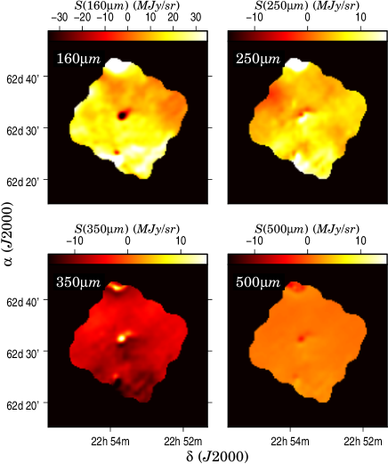
Figure 13: Residual maps of the surface brightness in the field PCC288 at four wavelengths when observations were fitted with the spectral index as a free parameter. The resolution is 1 arc minute.

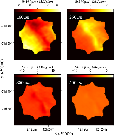
Figure 14: Residual maps of the surface brightness in the field PCC550 at four wavelengths.

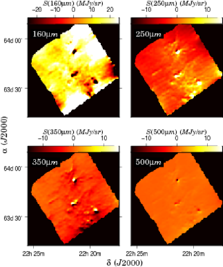
Figure 15: Residual maps of the surface brightness in the field PCC249 at the four wavelengths.

B.1 Maps of the spectral index uncertainty

The derived spectral index values are affected by observational noise, errors in the zero point of the adopted surface brightness scale, and errors in the gain calibration. Figure 16 shows maps that can be used to assess the importance of gain calibration and zero point errors. As discussed in Sect. 3.3, we modified the 250 $\mu$m and 500 $\mu$m surface brightness maps by adding or subtracting the zero point uncertainties from Table 2 and by scaling the maps by an amount corresponding to a 10% gain uncertainty. The changes at the two wavelengths were made in opposite directions in order to have the maximum effect in the $\beta$ value. By applying 1$\sigma$ shifts in the gain and in the offset and at both wavelengths critical for the determination of the spectral index we should get conservative limits for the spectral indices. The maps of minimum and maximum spectral indices are shown in Fig. 16.

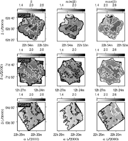
Figure 16: Estimated uncertainty of the spectral index maps. The first column shows the derived values (as in Fig. 4). The second and the third columns show the minimum and maximum values of $\beta$ consistent the estimated zero point uncertainties and an error of 10% in the gain calibration. The contours are drawn between 1.4 and 2.9 in steps of 0.3 units (white contours starting with value 2.3).

B.2 Temperature and spectral index maps without 100 $\mu$m data

The subtraction of the VSG emission from the 100 $\mu$m data relied on the ratio of the VSG and BG grains in the Désert et al. (Desert1990 (1990)) dust model. This also affects the 160 $\mu$m data but only as an uncertainty of the zero point of the intensity scale. To check to what extent the colour temperature and the spectral index maps are influenced by the 100 $\mu$m data, we recomputed the parameters using the 160 $\mu$m–500 $\mu$m data only. The resulting maps of the colour temperature and the spectral index are shown in Fig. 17.

The maps are morphologically similar to those shown in Fig. 4. The largest differences are in PCC550 where, without the 100 $\mu$m data, the spectral index map closely follows the shape of the dense filament. The appearance of SW part of that map again suggests the presence of some artifact, the $\beta$ values decreasing close to one. Compared to Fig. 4, PCC249 exhibits somewhat lower values of $\beta$ and a higher range of temperatures.

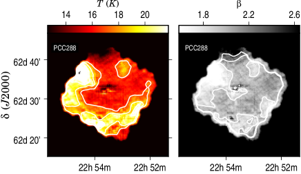
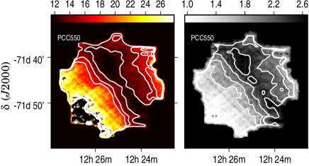
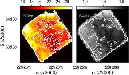
Figure 17: The colour temperature and dust spectral index map obtained by fitting the observations between 160 $\mu$m and 500 $\mu$m.

- (1) Anderson, L.D., Zavagno, A., Rodón, J.A., et al. 2010, A&A 518, L99
- (2) André, P., Men’shchikov, A., Bontemps, S., et al. 2010, A&A 518, L102
- (3) deAvillez, M., Breitschwerdt, D., 2007, ApJ 665, L35
- (4) Bally, J., Reipurth, B., Walawender, J., Armond, T. 2002, AJ 124, 2152
- (5) Bergin, E.A., Tafalla, M. 2007, ARA&A 45, 339
- (6) Bohlin R.C., Savage B.D., Drake J.F., 1978, ApJ 224, 132
- (7) Bonnor, W. B. 1956, MNRAS, 116, 351
- (8) Boudet, N., Mutschke, H., Nayral, C., et al., 2005, ApJ 633, 272
- (9) Boulanger, F., Abergel, A., Bernard J.-P., et al., 1996, A&A 312, 256
- (10) Compiègne, M., Verstraete, L., Jones, A., et al. 2011, A&A 525, 103
- (11) Crampton, D., Fisher, W.A. 1974, Pub.Dom.Astrophys.Obs., 4, 283
- (12) Crapsi, A., Caselli, P., Walmsley, C.M., Tafalla, M. 2007, A&A 470, 221
- (13) Crutcher, R.M., Hakobian, N., Troland, T.H. 2009, ApJ 692, 844
- (14) Désert, F.-X., Boulanger, F., Puget, J.L. 1990, A&A 237, 215
- (15) Désert, F.-X., Macías-Pérez, J. F., Mayet, F., et al. 2008, A&A 481, 411
- (16) Dobashi, K., Uehara, H., Kandori, R., et al. 2005, PASJ 57, S1
- (17) Draine, B., 2003, ApJ 598, 1017
- (18) Dupac, X., Bernard, J.-P., Boudet, N., et al. 2003, A&A, 404, L11
- Enoch et al. (2008) Enoch, M. L., Evans, N. J., Sargent, A. I., et al. 2008, ApJ, 684, 1240
- (20) Evans, N.J. II., Dunham, M.M., Jørgensen, J.K., et al. 2009, ApJS 181, 321
- (21) Goodman, A., Rosolowsky, E.W., Borkin, M.A., et al. 2009, Nature 457, 63
- (22) Griffin, M., Abergel, A., Abreu, A., et al. 2010, A&A 518, 3
- (23) Harju J., Juvela M., Schlemmer S., et al., 2008, A&A 482, 535
- (24) Hill, T., Thompson, M.A., Burton, M.G., et al. 2006, MNRAS, 368, 1223
- (25) Hirota, T., Ando, K., Bushimata, T., et al. 2008, PASJ 60, 961
- Johnstone et al. (2000) Johnstone, D., Wilson, C. D., Moriarty-Schieven, G., et al. 2000, ApJ, 545, 327
- (27) Jordi, C., Trullols, E., Galadi-Enriquez, D. 1996 A&A 312, 499
- (28) Juvela, M., Padoan, P., 2003, A&A 397, 201
- (29) Juvela, M., Pelkonen, V.-M., Porceddu, S. 2009, A&A 505, 663
- (30) Juvela, M., Ristorcelli, I., Montier, L.A. et al. 2010, A&A 518, L93
- (31) Kramer, C., Richer, J., Mookerjea, B., Alves J., Lada C., et al., 2003, A&A 399, 1073
- (32) Kramer, C., Alves, J., Lada, C.J., et al. 1999, A&A 342, 257
- (33) Krügel, E., Siebenmorgen, R., 1994, A&A 288, 929
- (34) Lombardi, M. & Alves, J., 2001, A&A 377, 1023
- (35) Malinen, J., Juvela, M., Collins, D., Lunttila, T., Padoan, P. 2011, submitted, arXiv:1009.4580
- (36) Mathis, J.S., Mezger, P.G., Panagia, N., 1983, A&A, 128, 212
- (37) McKee, C.F., Ostriker, E.C. 2007, ARA&A 45, 565
- (38) Mennella, V., Brucato, J.R., Colangeli, L., et al., 1998, ApJ 496, 1058
- (39) Mény, C., Gromov, V., Boudet, N., et al. 2007, A&A, 468, 171
- (40) Miville-Deschn̂es, M.-A., Lagache, G. 2005, ApJS 157, 302
- (41) Montier, L., Pelkonen V.-M., Juvela, M., Ristorcelli, I., Marshall, D. 2010, A&A 522, 83
- (42) Motte, F., Andre, P., & Neri, R. 1998, A&A, 336, 150
- (43) Motte, F., Andre, P., Ward-Thompson, D., et al. 2001, A&A, 372, 41
- (44) Nutter, D., Ward-Thompson, D-, Andreé, P. 2006, MNRAS 368, 1833
- (45) Nutter, D., Kirk, J.M., Stamatellos, D., Ward-Thompson, D., 2008, MNRAS 384, 755
- (46) Ossenkopf, V., & Henning, Th. 1994, A&A, 291, 943
- (47) Padoan, P., Jimenez, R., Nordlund, Å., Boldyrev, S. 2004, Phys. Rev. Lett., 92, 1102
- (48) Palla, F., Brand, J., Comoretto, G., Felli, M., Cesaroni, R. 1991, A&A, 246, 249
- (49) Piat, M., Lagache, G., Bernard, J.P., et al. 2002, A&A 393, 359
- (50) Pilbratt, G., Riedinger, J., Passvogel, T., et al. 2010, A&A 518, L1
- (51) Planck Collaboration 2011a, submitted, arXiv:1101.2035
- (52) Planck Collaboration 2011b, submitted, arXiv:1101.2034
- (53) Poglitsch, A., Waelkens, C., Geis, N., et al. 2010, A&A 518, 2
- (54) Reipurth, B., Aspin, C., Beck, T. et al. 2007, AJ 133 1000
- (55) Rodón, J.A., Zavagno, A., Baluteau, J.-P., et al. 2010, A&A 518, 80
- (56) Sargent, A.I. 1977, ApJ 218, 736
- (57) Schwartz, P.R. 1982, ApJ 252, 589
- (58) Sharpless, S. 1959, ApJS 4, 257
- (59) Schlegel, D.J., Finkbeiner, D.P., Davis, M., 1998, ApJ 500, 525
- (60) Shetty, R., Kauffmann, J., Schnee, S., & Goodman, A. A. 2009a, ApJ, 696, 676
- (61) Shetty, R., Kauffmann, J., Schnee, S., Goodman, A. A., & Ercolano, B. 2009b, ApJ, 696, 2234
- (62) Shetty, R., Collins, D. C., Kauffmann, J., Goodman, A. A., Rosolowsky, E. W., & Norman, M. 2010, The Astrophysical Journal, 712, 1049
- (63) Skrutskie, M.F., Cutri, R.M., Stiening, R., et al. 2006, AJ 131, 1163
- (64) Steinacker, J., Pagani, L., Backmann, A., Guieu, S. 2010, A&A 511, 9
- (65) Stepnik, B., Abergel, A., Bernard, J.-P. et al., 2003, A&A 398, 551
- (66) Tafalla, M., Bachiller, R., Martń-Pintado, J. 1993, ApJ 403, 175
- (67) Tauber, J., Mandolesi, N., Puget, J.-L., et al. 2010 (accepted)
- (68) Veneziani, M., Ade, P.A.R., Bock, J.J., et al. ApJ, 2010, 713, 959
- (69) Vilas-Boas, J.W.S., Myers, P.C., Fuller, G.A. 1993, ApJ 433, 96
- (70) Ward-Thompson, D., André, P., Crutcher, R., et al. 2007, in Protostars and Planets V, ed. B. Reipurth, D. Jewitt, K. Keil, 33
- (71) Wang, k., Wu, Y.F., Ran, L., Yu, W.T., Miller, M. 2009, A&A 507, 369
- (72) Zhang, Q., Hunter, T.R., Brand, J. 2005, ApJ 625, 864
- (73) Zinnecker, H., Yorke, H.W. 2007, ARA&A 45, 481