Multiple Meixner-Pollaczek polynomials
and the six-vertex model

Abstract

We study multiple orthogonal polynomials of Meixner-Pollaczek type with respect to a symmetric system of two orthogonality measures. Our main result is that the limiting distribution of the zeros of these polynomials is one component of the solution to a constrained vector equilibrium problem. We also provide a Rodrigues formula and closed expressions for the recurrence coefficients. The proof of the main result follows from a connection with the eigenvalues of block Toeplitz matrices, for which we provide some general results of independent interest.

The motivation for this paper is the study of a model in statistical mechanics, the so-called six-vertex model with domain wall boundary conditions, in a particular regime known as the free fermion line. We show how the multiple Meixner-Pollaczek polynomials arise in an inhomogeneous version of this model.

Keywords: multiple orthogonal polynomial, Meixner-Pollaczek polynomial, recurrence relation, block Toeplitz matrix, potential theory, six-vertex model.

1 Introduction

In this paper we study a system of polynomials, orthogonal with respect to two different weight functions of Meixner-Pollaczek type. Our work is motivated by the analysis of the six-vertex model in statistical mechanics introduced in [24] and studied in many papers since then, see e.g. [3, 21, 20, 24, 28, 25, 38]. Colomo and Pronko [10, 11] studied the role of orthogonal polynomials in the six-vertex model, and in particular the Meixner-Pollaczek polynomials. An object of major physical interest is the partition function of this model. A rather complete analysis of the large $n$ asymptotics in the homogeneous case is based on the analysis of a Riemann-Hilbert problem for orthogonal polynomials [6, 7, 8, 9]. In the inhomogeneous case, the corresponding reasoning leads to questions of asymptotics of multiple orthogonal polynomials, as we will discuss in Section 2.4.

Here we will focus on a particular regime of the six-vertex model, known as the “free fermion line”. In the homogeneous case, this case is trivial, the partition function being identically $1$. Also in the inhomogeneous case, a closed expression for the partition function can be calculated explicitly, so the present results do not give any new insights into the original model, but should rather be considered as providing exact and asymptotic information in its own right on the associated polynomials, the multiple Meixner-Pollaczek polynomials.

An important tool in the study of (usual) orthogonal polynomials $P_{n}$ on the real line, appropriately scaled in order to have $n$-dependent weights, is that their limiting zero distribution satisfies an equilibrium problem. This equilibrium problem is an important ingredient for the steepest descent analysis of the Riemann-Hilbert problem for orthogonal polynomials, thereby allowing to obtain strong and uniform asymptotics of the polynomials, see e.g. [15, 16].

For the case of multiple orthogonal polynomials, however, no general result is known about the existence of an equilibrium problem. The aim of this paper is to obtain such an equilibrium problem for multiple Meixner-Pollaczek polynomials. The equilibrium problem will be posed in terms of a couple of measures $(\nu_{1},\nu_{2})$ and it involves both an external source acting on $\nu_{1}$ and a constraint acting on $\nu_{2}$. This structure is very similar to the equilibrium problem for the GUE with external source model, [5].

Our method for obtaining the equilibrium problem is similar to that applied to other systems of multiple orthogonal polynomials [18, 26], but a distinguishing feature is the characterization in terms of the eigenvalue distributions of block Toeplitz matrices, rather than usual (scalar) Toeplitz matrices. We will provide some general results on this topic that are of independent interest. Along the way we also obtain Rodrigues formulae and closed expressions for the recurrence coefficients for multiple Meixner-Pollaczek polynomials.

Inspired by the scalar case [15, 16], one might hope that the equilibrium problem presented in this paper can be used in the steepest descent analysis of the Riemann-Hilbert problem for multiple Meixner-Pollaczek polynomials, thereby obtaining strong and uniform asymptotics for these polynomials. This approach, although interesting, will not be carried out in this paper. We also hope that our equilibrium problem might serve as an inspiration to obtain similar results for the general inhomogeneous six-vertex model, not necessarily on the free fermion line, which in turn could serve as the first step in finding the large $n$ asymptotic analysis for this model.

2 Statement of results

2.1 Multiple Meixner-Pollaczek polynomials

Let $w_{1}$ and $w_{2}$ denote two distinct weight functions of Meixner-Pollaczek type; $w_{j}:\mathbb{R}\to\mathbb{R}^{+}$ with

$$w_{j}(x)=\frac{1}{2\pi}e^{2t_{j}x}\left|\Gamma\left(\lambda+ix\right)\right|^{2},\quad j=1,2,$$ (2.1)

where $t_{1},t_{2}\in(-\pi/2,\pi/2)$, $t_{1}\neq t_{2}$ and $\lambda>0$ are fixed parameters and $\Gamma$ denotes Euler’s gamma function [1]. Note that in (2.1) the gamma function is evaluated in a complex argument and that

$$\left|\Gamma\left(\lambda+ix\right)\right|^{2}=\Gamma\left(\lambda+ix\right)\Gamma\left(\lambda-ix\right),\quad\textrm{for any }\lambda,x\in\mathbb{R}.$$

Furthermore, for $\lambda$ fixed, $\left|\Gamma\left(\lambda+ix\right)\right|^{2}\sim e^{-\pi|x|}$ as $|x|\to\infty$, so the restrictions on $t_{j}$ guarantee that $w_{j}$ is exponentially decaying for $x\to\pm\infty$.

Lemma 2.1.

(Existence, uniqueness, real and interlacing zeros) For any nonnegative integers $k_{1}$ and $k_{2}$, there is a unique monic polynomial $P_{k_{1},k_{2}}$ of degree $k=k_{1}+k_{2}$ satisfying the orthogonality conditions

$$\int_{-\infty}^{\infty}P_{k_{1},k_{2}}(x)x^{m}w_{j}(x)\mathrm{d}x=0,\quad\textrm{ for }m=0,\ldots,k_{j}-1,\quad j=1,2.$$

The zeros of these polynomials are real and interlacing, in the sense that each $P_{k_{1},k_{2}}$ has $k$ distinct real zeros $x_{1}^{k_{1},k_{2}}<x_{2}^{k_{1},k_{2}}<\cdots<x_{k}^{k_{1},k_{2}}$ such that $x_{j}^{k_{1},k_{2}}<x_{j}^{k_{1}-1,k_{2}}<x_{j+1}^{k_{1},k_{2}}$ and $x_{j}^{k_{1},k_{2}}<x_{j}^{k_{1},k_{2}-1}<x_{j+1}^{k_{1},k_{2}}$ whenever $1\leq j\leq k-1$.

Lemma 2.1 will be proved in Section 3.1.

In analogy with the case of Meixner-Pollaczek orthogonal polynomials [23] we refer to the $P_{k_{1},k_{2}}$ as multiple Meixner-Pollaczek polynomials; see also [4, Sec. 4.3.3]. These polynomials are related to the six-vertex model; see Section 2.4. For information on other systems of multiple orthogonal polynomials in the literature, see e.g. [2, 34].

In this paper we will derive a Rodrigues type formula for the polynomials $P_{k_{1},k_{2}}$, enabling us to compute explicitly the following four term recurrence relations, to be proved in Section 3.

Theorem 2.2.

(Recurrence relations) Let $t_{1},t_{2}\in(-\pi/2,\pi/2)$ with $t_{1}\neq t_{2}$. Then, for nonnegative integers $k_{1}$ and $k_{2}$, the multiple Meixner-Polleczek polynomials satisfy the recurrence relations

$$P_{k_{1}+1,k_{2}}(x)=\left(x-a_{k_{1},k_{2}}^{t_{1},t_{2}}\right)P_{k_{1},k_{2}}(x)-b_{k_{1},k_{2}}^{t_{1},t_{2}}P_{k_{1},k_{2}-1}(x)-c_{k_{1},k_{2}}^{t_{1},t_{2}}P_{k_{1}-1,k_{2}-1}(x),$$ (2.2)

and

$$P_{k_{1},k_{2}+1}(x)=\left(x-a_{k_{2},k_{1}}^{t_{2},t_{1}}\right)P_{k_{1},k_{2}}(x)-b_{k_{2},k_{1}}^{t_{2},t_{1}}P_{k_{1}-1,k_{2}}(x)-c_{k_{2},k_{1}}^{t_{2},t_{1}}P_{k_{1}-1,k_{2}-1}(x),$$ (2.3)

where

$$a_{k_{1},k_{2}}^{t_{1},t_{2}}=\frac{(k+k_{1}+2\lambda)}{2}\tan t_{1}+\frac{k_{2}}{2}\tan t_{2},$$

$$b_{k_{1},k_{2}}^{t_{1},t_{2}}=\frac{(k+2\lambda-1)}{4}\left(\frac{k_{1}}{\cos^{2}\!t_{1}}+\frac{k_{2}}{\cos^{2}\!t_{2}}\right),$$

$$c_{k_{1},k_{2}}^{t_{1},t_{2}}=\frac{k_{1}(k+2\lambda-1)(k+2\lambda-2)(\tan t_{1}-\tan t_{2})}{8\cos^{2}\!t_{1}},$$

$k=k_{1}+k_{2}$, and where we set $P_{-1,k_{2}}\equiv 0$, $P_{k_{1},-1}\equiv 0$ for any $k_{1},k_{2}$.

The above theorem is the basis for the main purpose of the paper, namely to study the asymptotic zero distribution of the appropriately rescaled multiple Meixner-Pollaczek polynomials. Fix $t_{1}$ and $t_{2}$. For simplicity we choose a particular sequence of indices $(k_{1}(k),k_{2}(k))_{k=1}^{\infty}$ along which we analyze the large $k$ asymptotics of $P_{k_{1}(k),k_{2}(k)}$, and form the single sequence

$$Q_{k}(x)=\left\{\begin{array}[]{ll}P_{k/2,k/2}(x)&\textrm{ if $k$ is even,}\\ P_{(k+1)/2,(k-1)/2}(x)&\textrm{ if $k$ is odd,}\end{array}\right.$$

of polynomials. We will show that the zero-distribution of the rescaled polynomials $Q_{k}(kx)$ has a weak limit as $k$ goes to infinity, and in order to study this we let $n\in\mathbb{N}$ and introduce the doubly indexed sequence of monic polynomials $\{Q_{k,n}\}_{k\geq 0}$ defined by

$$Q_{k,n}(x)=\frac{1}{n^{k}}Q_{k}(nx).$$

From (2.2) and (2.3) we obtain an explicit recurrence relation for $Q_{k,n}$,

$$xQ_{k,n}(x)=Q_{k+1,n}(x)+a_{k,n}Q_{k,n}(x)+b_{k,n}Q_{k-1,n}(x)+c_{k,n}Q_{k-2,n}(x),$$ (2.4)

with initial conditions $Q_{-3,n}\equiv Q_{-2,n}\equiv Q_{-1,n}\equiv 0$, where

$$\left\{\begin{array}[]{lll}\displaystyle a_{k,n}=\frac{1}{n}a_{k/2,k/2}^{t_{1},t_{2}}=\frac{3k+4\lambda}{4n}\tan t_{1}+\frac{k}{4n}\tan t_{2}\\ \displaystyle b_{k,n}=\frac{1}{n^{2}}b_{k/2,k/2}^{t_{1},t_{2}}=\frac{k(k+2\lambda-1)}{8n^{2}}\left(\frac{1}{\cos^{2}\!t_{1}}+\frac{1}{\cos^{2}\!t_{2}}\right)\\ \displaystyle c_{k,n}=\frac{1}{n^{3}}c_{k/2,k/2}^{t_{1},t_{2}}=\frac{k(k+2\lambda-1)(k+2\lambda-2)}{16n^{3}}\frac{(\tan t_{1}-\tan t_{2})}{\cos^{2}\!t_{1}}\end{array}\right.$$ (2.5)

for $k$ even and

$$\left\{\begin{array}[]{lll}a_{k,n}=\displaystyle\frac{1}{n}a_{(k-1)/2,(k+1)/2}^{t_{2},t_{1}}=\frac{k+1}{4n}\tan t_{1}+\frac{3k+4\lambda-1}{4n}\tan t_{2}\\ b_{k,n}=\displaystyle\frac{1}{n^{2}}b_{(k-1)/2,(k+1)/2}^{t_{2},t_{1}}=\frac{k+2\lambda-1}{8n^{2}}\left(\frac{k+1}{\cos^{2}\!t_{1}}+\frac{k-1}{\cos^{2}\!t_{2}}\right)\\ c_{k,n}=\displaystyle\frac{1}{n^{3}}c_{(k-1)/2,(k+1)/2}^{t_{2},t_{1}}=\frac{(k-1)(k+2\lambda-1)(k+2\lambda-2)}{16n^{3}}\frac{(\tan t_{2}-\tan t_{1})}{\cos^{2}\!t_{2}}\end{array}\right.$$ (2.6)

for $k$ odd.

Using the recurrence relation (2.4), standard considerations show that the zeros of $Q_{n,n}$ are the eigenvalues of the $4$-diagonal matrix

$$\left(\begin{array}[]{ccccc}a_{0,n}&1&&&0\\ b_{1,n}&a_{1,n}&1&&\\ c_{2,n}&b_{2,n}&a_{2,n}&\ddots&\\ &\ddots&\ddots&\ddots&1\\ 0&&c_{n-1,n}&b_{n-1,n}&a_{n-1,n}\end{array}\right)_{n\times n}.$$ (2.7)

So the problem of the asymptotic zero-distribution of $Q_{n,n}$ reduces to finding the eigenvalue asymptotics of (2.7). If $k$ and $n$ both tend to infinity in such a way that $k/n\to s$ for some constant $s$, then the coefficients $a_{k,n}$ have two subsequential limits $a_{s}$ and $\tilde{a}_{s}$ for even and odd $k$ respectively. Similarly, $b_{k,n}$ and $c_{k,n}$ have subsequential limits $b_{s},c_{s}$ and $\tilde{b}_{s},\tilde{c}_{s}$ along subsequences consisting of even and odd $k$ respectively. Using the identity $1/\cos^{2}\!t=1+\tan^{2}\!t$, these limits become

$$\left\{\begin{array}[]{l}a_{s}=\left(3\tan t_{1}+\tan t_{2}\right)s/4\\ b_{s}=\left(2+\tan^{2}\!t_{1}+\tan^{2}\!t_{2}\right)s^{2}/8\\ c_{s}=(\tan t_{1}-\tan t_{2})(1+\tan^{2}\!t_{1})s^{3}/{16},\end{array}\right.$$ (2.8)

$$\left\{\begin{array}[]{l}\tilde{a}_{s}=\left(3\tan t_{2}+\tan t_{1}\right)s/4\\ \tilde{b}_{s}=b_{s}\\ \tilde{c}_{s}=(\tan t_{2}-\tan t_{1})(1+\tan^{2}\!t_{2})s^{3}/{16}.\end{array}\right.$$ (2.9)

If we consider (2.7) in $2\times 2$ blocks, it is tri-diagonal with blocks

$$A^{(-1)}_{k,n}=\left(\begin{array}[]{cc}0&0\\ 1&0\end{array}\right),$$

$$A^{(0)}_{k,n}=\begin{pmatrix}a_{2k,n}&1\\ b_{2k+1,n}&a_{2k+1,n}\end{pmatrix},$$

and

$$A^{(1)}_{k,n}=\begin{pmatrix}c_{2k,n}&b_{2k,n}\\ 0&c_{2k+1,n}\end{pmatrix}.$$

In view of the limits (2.5) and (2.6), the blocks are slowly varying along the diagonals if $n$ is large. In other words, for large $n$, the matrix (2.7) has a locally block Toeplitz structure with square blocks of size $r=2$. This allows its limiting eigenvalue distribution to be obtained from a general machinery to which we turn now.

2.2 Polynomials generated by a general recurrence relation

In this subsection we will work in the following general setting. Let $n$ be a fixed parameter and let $(Q_{k,n}(x))_{k=0}^{\infty}$ be a sequence of monic polynomials, where $Q_{k,n}$ has degree $k$ and depends parametrically on $n$. Assume that the $Q_{k,n}$ are generated by the recurrence relation

$$x\begin{pmatrix}Q_{0,n}(x)\\ Q_{1,n}(x)\\ \vdots\end{pmatrix}=J_{n}\begin{pmatrix}Q_{0,n}(x)\\ Q_{1,n}(x)\\ \vdots\end{pmatrix},$$ (2.10)

where $J_{n}$ is a semi-infinite matrix with unit lower Hessenberg structure, i.e., the strictly upper triangular part of $J_{n}$ is equal to zero, except for the first superdiagonal, on which all entries are $1$. We also assume that the lower triangular part of $J_{n}$ has a finite bandwidth, which is independent of $n$.

The entries of $J_{n}$ are assumed to have asymptotically periodic behavior with period $r$ ($r\geq 1$). More precisely, suppose $J_{n}$ is partitioned into blocks of size $r\times r$, with one superdiagonal and a fixed finite number $\beta$ of subdiagonal non-zero blocks,

$$J_{n}=\left(A_{k,n}^{(k-l)}\right)_{k,l=0}^{\infty}=\begin{pmatrix}A_{0,n}^{(0)}&A_{0,n}^{(-1)}&0&\cdots\\ A_{1,n}^{(1)}&A_{1,n}^{(0)}&A_{1,n}^{(-1)}&\ddots\\ \vdots&\ddots&\ddots&\ddots\\ \vdots&\vdots&\vdots&\vdots\\ \vdots&\ddots&&\\ A_{\beta,n}^{(\beta)}&A_{\beta,n}^{(\beta-1)}&A_{\beta,n}^{(\beta-2)}&\\ 0&A_{\beta+1,n}^{(\beta)}&A_{\beta+1,n}^{(\beta-1)}&\ddots\\ \vdots&\ddots&\ddots&\ddots\end{pmatrix},$$ (2.11)

where

$$A_{k,n}^{(-1)}=\begin{pmatrix}0&0&\cdots&0\\ \vdots&\vdots&&\vdots\\ 0&0&\cdots&0\\ 1&0&\cdots&0\\ \end{pmatrix}_{r\times r},\qquad A_{k,n}^{(0)}=\begin{pmatrix}*&1&&0\\ \vdots&&\ddots&\\ *&&&1\\ *&*&\cdots&*\\ \end{pmatrix}_{r\times r},$$ (2.12)

where the $*$’s denote arbitrary constants.

We will assume that the block entries $A_{k,n}^{(j)}$ in (2.11) are slowly varying with $n$, in the sense that the limits

$$\lim_{rk/n\to s}A_{k,n}^{(j)}=A^{(j)}_{s}$$ (2.13)

exist for any $j=-1,0,\ldots,\beta$ and $s\geq 0$. Here the notation $\lim_{rk/n\to s}$ means that we let both $k$ and $n$ tend to infinity, in such a way that the ratio $rk/n$ tends to a limit $s\geq 0$. The relation (2.13) is on the level of $r\times r$ matrices, with the limit taken entry-wise. If (2.13) holds then the matrix in (2.11) is said to have locally block Toeplitz structure, in the spirit of [33].

For fixed $s$, we collect the limiting matrices in (2.13) into the following matrix-valued Laurent polynomial $A_{s}(z)$:

$$A_{s}(z):=A_{s}^{(-1)}z^{-1}+A_{s}^{(0)}+\cdots+A_{s}^{(\beta)}z^{\beta}.$$ (2.14)

We will sometimes refer to $A_{s}(z)$ as the symbol. From (2.12)–(2.14) it follows that

$$A_{s}(z)=\begin{pmatrix}*&1&&0\\ \vdots&&\ddots&\\ *&&&1\\ (z^{-1}+*)&*&\cdots&*\\ \end{pmatrix}+\mathcal{O}(z),$$ (2.15)

where $\mathcal{O}(z)$ denotes all the terms in (2.14) that tend to zero as $z\to 0$.

Define for each $s\geq 0$, the algebraic equation

$$f_{s}(z,x):=\det(A_{s}(z)-xI_{r})=0,$$ (2.16)

where $I_{r}$ denotes the identity matrix of size $r$. Note that $f_{s}$ depends on two complex variables $z$ and $x$. By expanding the determinant (2.16) and using (2.15), we can write $f_{s}$ as a (scalar) Laurent polynomial in $z$:

$$f_{s}(z,x)=f_{-1,s}(x)z^{-1}+f_{0,s}(x)+\cdots+f_{p,s}(x)z^{p},$$ (2.17)

where $f_{j,s}(x)$, $j=-1,0,\ldots,p$, are polynomials in $x$, with $f_{-1,s}(x)\equiv(-1)^{r-1}$. We define $p$ in (2.17) as the largest positive integer for which $f_{p,s}\not\equiv 0$.

Let us solve (2.16) for $z$; this yields $p+1$ roots

$$z_{j}=z_{j}(x,s),\qquad j=1,\ldots,p+1.$$

We assume that for each $x\in\mathbb{C}$ these roots are ordered such that

$$0<|z_{1}(x,s)|\leq|z_{2}(x,s)|\leq\cdots\leq|z_{p+1}(x,s)|.$$ (2.18)

If $x\in\mathbb{C}$ is such that two or more consecutive roots in (2.18) have the same absolute value, then we arbitrarily label them so that (2.18) is satisfied.

Define the set

$$\Gamma_{1}(s)=\{x\in\mathbb{C}\mid|z_{1}(x,s)|=|z_{2}(x,s)|\}.$$ (2.19)

In the cases we are interested in, we will have that

$$\Gamma_{1}(s)\subset\mathbb{R}.$$ (2.20)

Supposing this to hold, we define a measure $\mu_{1}^{s}$ on $\Gamma_{1}(s)\subset\mathbb{R}$ with density

$$\mathrm{d}\mu_{1}^{s}(x)=\frac{1}{r}\frac{1}{2\pi i}\left(\frac{z_{1+}^{\prime}(x,s)}{z_{1+}(x,s)}-\frac{z_{1-}^{\prime}(x,s)}{z_{1-}(x,s)}\right)\mathrm{d}x.$$ (2.21)

Here the prime denotes the derivative with respect to $x$, and $z_{1\pm}(x,s)$ are the boundary values of $z_{1}(x,s)$ obtained from the $+$-side (upper side) and $-$-side (lower side) respectively of $\Gamma_{1}(s)\subset\mathbb{R}$. These boundary values exist for all but a finite number of points.

As discussed in [17], the measure $\mu_{1}^{s}$ can be interpreted as the weak limit as $n\to\infty$ of the normalized eigenvalue counting measures for the block Toeplitz matrices $T_{n}(A_{s})$ associated to the symbol (2.14).

Lemma 2.3.

With the above notation, we have

• $z_{1}(x,s)=x^{-r}+\mathcal{O}\left(x^{-r-1}\right)$ as $x\to\infty$.

• $\mu_{1}^{s}$ in (2.21) is a Borel probability measure on $\Gamma_{1}(s)$.

Proof.

See [17]. ∎

With this notation in place, let us return to the sequence of polynomials $(Q_{k,n})_{k=0}^{\infty}$ in (2.10). This sequence is said to have real and interlacing zeros if each $Q_{k,n}$ has $k$ distinct real zeros $x_{1}^{k,n}<x_{2}^{k,n}<\cdots<x_{k}^{k,n}$ such that $x_{j}^{k,n}<x_{j}^{k-1,n}<x_{j+1}^{k,n}$ whenever $1\leq j\leq k-1$.

The next result states that, under certain conditions, the normalized zero-counting measures of the polynomials $Q_{n,n}$ have a (weak) limit for $n\to\infty$, which is precisely the average of the measures (2.21). Here the average is with respect to the parameter $s$.

Theorem 2.4.

(Limiting zero distribution of $Q_{n,n}$) Let the sequence of polynomials $(Q_{k,n})_{k=0}^{\infty}$ be such that (2.10)–(2.13) hold. Assume that $(Q_{k,n})_{k=0}^{\infty}$ has real and interlacing zeros for each $n$, as described above. Also assume that (2.20) holds for every $s\geq 0$. Then as $n\to\infty$, the normalized zero-counting measure $\rho_{n}$ of the polynomial $Q_{n,n}$,

$$\rho_{n}:=\frac{1}{n}\sum_{j=1}^{n}\delta_{x_{j}^{n,n}},$$ (2.22)

where $\delta_{z}$ denotes the Dirac point mass at $z$, has the limit

$$\lim_{n\to\infty}\rho_{n}=\nu_{1}:=\int_{0}^{1}\mu_{1}^{s}\,\mathrm{d}s$$ (2.23)

in the sense of weak convergence of measures, where $\mu_{1}^{s}$ is defined in (2.21).

Theorem 2.4 will be proven in Section 4. This theorem generalizes a result for the scalar case $r=1$ by Kuijlaars-Román [26, Theorem 1.2]; see also [14, 27].

2.3 Zeros of multiple Meixner-Pollaczek polynomials

We apply Theorem 2.4 to the polynomials $Q_{k,n}$ in Section 2.1. In what follows, we will assume the condition of symmetric weights,

$$t:=t_{1}=-t_{2};$$

for this case we can characterize the limiting zero distribution in terms of a constrained vector equilibrium problem, Theorem 2.6, which is the main result of the paper. The symmetry condition in Proposition 2.5 is needed to prove that $\Gamma_{1}(s)\subset\mathbb{R}$; in the general case this may fail.

The recurrence coefficients in (2.8) and (2.9) then become

$$\left\{\begin{aligned} a_{s}&=&-\tilde{a}_{s}&=(\tan t)s/2,\\ b_{s}&=&\tilde{b}_{s}&=(1+\tan^{2}\!t)s^{2}/4,\\ c_{s}&=&-\tilde{c}_{s}&=\tan t(1+\tan^{2}\!t)s^{3}/8=a_{s}b_{s}.\end{aligned}\right.$$ (2.24)

We partition the matrix $J_{n}$ from (2.7) into blocks as in (2.11) with $r=2$ and $\beta=1$. Then the limiting values in (2.13) exist and are given by

$$A^{(-1)}_{s}=\begin{pmatrix}0&0\\ 1&0\end{pmatrix},$$

$$A^{(0)}_{s}=\begin{pmatrix}a_{s}&1\\ b_{s}&-a_{s}\end{pmatrix},$$

and

$$A^{(1)}_{s}=\begin{pmatrix}c_{s}&b_{s}\\ 0&-c_{s}\end{pmatrix},$$

with $a_{s}$, $b_{s}$ and $c_{s}$ as in (2.24). The symbol $A_{s}(z)$ in (2.14) now becomes

$$A_{s}(z)=A_{s}^{(-1)}z^{-1}+A_{s}^{(0)}+A_{s}^{(1)}z=\begin{pmatrix}a_{s}(1+b_{s}z)&1+b_{s}z\\ z^{-1}\left(1+b_{s}z\right)&-a_{s}(1+b_{s}z)\end{pmatrix},$$

so (2.16) reduces to

$$x^{2}-\frac{(1+b_{s}z)^{2}(1+a_{s}^{2}z)}{z}=0.$$ (2.25)

This equation has three roots, $z_{j}(x,s)$, $j=1,2,3$ which we label in order of increasing modulus:

$$0<|z_{1}(x,s)|\leq|z_{2}(x,s)|\leq|z_{3}(x,s)|.$$ (2.26)

Proposition 2.5.

(Limiting zero distribution) Suppose $t_{1}=-t_{2}=t\in(0,\pi/2)$. As $n\to\infty$, the normalized zero-counting measure $\rho_{n}$ of the multiple Meixner-Pollaczek polynomial $Q_{n,n}$ in Section 2.1, see (2.22), converges weakly to the average $\nu_{1}=\int_{0}^{1}\mu_{1}^{s}\,\mathrm{d}s$ of the measures $\mu_{1}^{s}$ in (2.21).

Proof.

This is a consequence of Theorem 2.4. The assumptions in the latter theorem are indeed satisfied: the interlacing condition follows from Lemma 2.1, and the fact that $\Gamma_{1}(s)\subset\mathbb{R}$ follows from Proposition 5.1. ∎

In addition to the set $\Gamma_{1}(s)$ in (2.19), we define

$$\Gamma_{2}(s)=\{x\in\mathbb{C}\mid|z_{2}(x,s)|=|z_{3}(x,s)|\}.$$ (2.27)

We will now characterize the limiting zero distribution $\nu_{1}$ in terms of a vector equilibrium problem from logarithmic potential theory [30, 31]. Recall that for a pair of Borel measures $(\mu,\nu)$ supported in the complex plane, the mixed logarithmic energy of $\mu$ and $\nu$ is defined as [31]

$$I(\mu,\nu):=\iint\log\frac{1}{|x-y|}\,\mathrm{d}\mu(x)\,\mathrm{d}\nu(y).$$

Theorem 2.6.

(Equilibrium problem) Suppose $t_{1}=-t_{2}=t\in(0,\pi/2)$. Then the asymptotic zero distribution, $\nu_{1}$, of $Q_{n,n}$ is the first component of the unique minimizer $(\nu_{1},\nu_{2})$ of the energy functional

$$E(\mu,\nu):=I(\mu,\mu)+I(\nu,\nu)-I(\mu,\nu)+\int(\pi-2t)|x|\,\mathrm{d}\mu(x),$$

among all vectors $(\mu,\nu)$ of positive measures such that $\operatorname{supp}\mu\subset\mathbb{R}$, $\int\,\mathrm{d}\mu=1$, $\operatorname{supp}\nu\subset i\mathbb{R}$, $\int\,\mathrm{d}\nu=1/2$ and $\nu$ is absolutely continuous with density satisfying

$$\frac{\mathrm{d}\nu(ix)}{|\mathrm{d}x|}\leq\frac{2t}{\pi}.$$

The measures have the properties

$$\operatorname{supp}\nu_{1}=[-c_{1},c_{1}]$$

and

$$\operatorname{supp}(\sigma-\nu_{2})=i\mathbb{R}\setminus(-ic_{2},ic_{2}),$$

where $\sigma$ is the positive, absolutely continuous measure on $i\mathbb{R}$ with constant density $\frac{2t}{\pi}$, and where $c_{1}$ and $c_{2}$ are positive constants given by

$$c_{1}=\left(\frac{27b^{4}+18b^{2}-1+\sqrt{b^{2}+1}(9b^{2}+1)^{3/2}}{32b^{2}}\right)^{1/2}$$ (2.28)

and

$$c_{2}=\left(\frac{\sqrt{b^{2}+1}(9b^{2}+1)^{3/2}-27b^{4}-18b^{2}+1}{32b^{2}}\right)^{1/2},$$ (2.29)

with

$$b=\tan t.$$

Furthermore, $\nu_{1}$ is absolutely continuous with respect to Lebesgue measure and has density

$$\frac{\mathrm{d}\nu_{1}}{\mathrm{d}x}=\frac{1}{2\pi}\log\left|\frac{1+iw(x)}{1-iw(x)}\right|,\qquad x\in[-c_{1},c_{1}],$$ (2.30)

where

$$w(x)=\frac{(4+z(b^{2}-1))(4+z(b^{2}+1))}{16z|x|}$$ (2.31)

and $z=z(x)$ is the complex solution to the algebraic equation

$$\frac{(4+z(b^{2}+1))^{2}(4+zb^{2})}{64z}=x^{2}$$ (2.32)

such that $\operatorname{Im}(w(x))<0$.

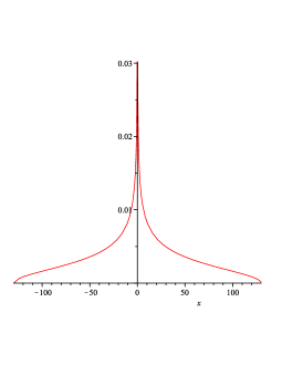
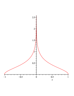
Figure 1: Density of the measure $\nu_{1}$ for (a) $b=\tan t=100$ and (b) $b=\tan t=0.1$.

Remark 2.7.

In general, there is no closed expression for the density of $\nu_{1}$, but in the limiting case $t\to 0$, corresponding to the ordinary Meixner-Pollaczek orthogonal polynomials, (2.32) can be explicitly solved, $z=8x^{2}-4+8i|x|\sqrt{1-x^{2}}$, giving $|z|=4$. Thus (2.31) becomes

$$w(x)=\frac{16-z^{2}}{16z|x|}=\frac{16\overline{z}-|z|^{2}z}{16|z|^{2}|x|}=-i\frac{\operatorname{Im}(z)}{8|x|}=-i\sqrt{1-x^{2}},$$

and the density (2.32) takes the form

$$\frac{\mathrm{d}\nu_{1}}{\mathrm{d}x}=\frac{1}{2\pi}\log\left(\frac{1+\sqrt{1-x^{2}}}{1-\sqrt{1-x^{2}}}\right)\chi_{\{|x|\leq 1\}}.$$ (2.33)

For non-zero values of $t\in(0,\pi/2)$, the density of $\nu_{1}$ turns out to have the same qualitative features as (2.33); see Figure 1 for some illustrations.

Theorem 2.6 will be proven in Section 5. The proof uses a general result for block Toeplitz matrices [17], see also [19], together with some explicit calculations using (2.25).

2.4 Motivation: The six-vertex model with domain wall boundary conditions

Multiple Meixner-Pollaczek polynomials appear in the study of the six-vertex model in statistical mechanics, as we explain now.

Consider an $N\times N$ square lattice in the plane. A configuration of the six-vertex model is an assignment of an orientation to the edges of the lattice in such a way that each vertex is surrounded by precisely two incoming and two outgoing edges. See Fig. 2 for a configuration with $N=5$. The name six-vertex model refers to the fact that the local behavior near each vertex is given by six possible edge configurations (see Fig. 3).

We consider the six-vertex model with domain wall boundary conditions (DWBC). This means that the edges at the top and bottom of the lattice must be directed outwards and those at the left and right of the lattice must be directed inwards.

Figure 2: A configuration of the six-vertex model with DWBC for $N=5$

Figure 3: Six types of vertices.

To each of the $N$ rows of the lattice we associate a parameter $x_{i}\in\mathbb{R}$ and similarly to each column a parameter $y_{j}\in\mathbb{R}$, $i,j=1,\ldots,N$. We also fix a positive parameter $\gamma$ and we assume that $|x_{i}-y_{j}|<\gamma$ for all $i$ and $j$. We define the weight of the vertex in row $i$ and column $j$ according to its type as $\sin(2\gamma)$ (type 1 or 2), $\sin(\gamma-(x_{i}-y_{j}))$ (type 3 or 4), or $\sin(\gamma+(x_{i}-y_{j}))$ (type 5 or 6). Note that the weights are parameterized according to the so-called disordered phase convention.

The weight of a configuration is defined as the product of the weights of all the $N\times N$ vertices in the configuration. The partition function $Z_{N}=Z_{N}(x_{1},\ldots,x_{N},y_{1},\ldots,y_{N},\gamma)$ is defined as the sum of the weights of all the consistent configurations of the $N\times N$ six-vertex model with DWBC. An explicit expression for the partition function in terms of an $N\times N$ determinant was found by Izergin and Korepin [20, 21], see also [3, 25, 28].

The homogeneous case

In the case where $x_{i}-y_{j}\equiv t$ for all $i,j=1,\ldots,N$, for some fixed parameter $t\in(-\gamma,\gamma)$, the Izergin-Korepin formula reduces to

$$Z_{N}=Z_{N}(\gamma,t)=\frac{[\sin(\gamma+t)\sin(\gamma-t)]^{N^{2}}}{\left(\displaystyle\prod_{n=0}^{N-1}n!\right)^{2}}\det M,$$ (2.34)

where the matrix $M=(m_{i,j})_{i,j=1}^{N}$ has entries

$$m_{i,j}=\int_{-\infty}^{\infty}x^{i+j-2}e^{tx}w(x)\ dx$$ (2.35)

with

$$w(x)=\frac{\sinh(\frac{x}{2}(\pi-2\gamma))}{\sinh(\frac{x}{2}\pi)},$$ (2.36)

see e.g. [6, 21, 38]. The matrix $M$ is then precisely the moment matrix corresponding to the weight function $e^{tx}w(x)$ on the real line. Standard considerations (e.g. [32]) show that $\det M$ can be expressed in terms of the monic orthogonal polynomials $P_{n}(x)$ defined by

$$P_{n}(x)=x^{n}+\mathcal{O}(x^{n-1})$$

for all $n$ and

$$\int_{-\infty}^{\infty}P_{n}(x)x^{m}e^{tx}w(x)\ \mathrm{d}x=h_{n}\delta_{m,n}$$ (2.37)

for all $n,m$ with $m\leq n$. In fact, $\det M$ is expressed in terms of the numbers $h_{n}$ in (2.37) through the formula

$$\det M=\prod_{n=0}^{N-1}h_{n}.$$ (2.38)

Special choices of parameters lead to known families of orthogonal polynomials. Indeed, Colomo and Pronko [10, 11] showed that the Continuous Hahn, Meixner-Pollaczek and continuous Dual Hahn polynomials appear in this way. In more general cases, the expressions (2.34)–(2.38) were used to compute the asymptotics of the partition function $Z_{N}$ for large $N$ in great detail by means of the Riemann-Hilbert method [6], see also [7, 8].

The inhomogeneous case

The situation in this paper corresponds to the case where

$$x_{i}-y_{j}\equiv\left\{\begin{array}[]{ll}t_{1},&1\leq i\leq n_{1},\\ t_{2},&n_{1}+1\leq i\leq n_{1}+n_{2}=N,\end{array}\right.$$ (2.39)

for some $t_{1}\neq t_{2}$ and all $j=1,\ldots,N$. Following the reasoning in [21], see also the appendix in [12], one sees that the Izergin-Korepin formula reduces to

$$Z_{N}=\frac{[\sin(\gamma+t_{1})\sin(\gamma-t_{1})]^{n_{1}N}[\sin(\gamma+t_{2})\sin(\gamma-t_{2})]^{n_{2}N}}{\left(\displaystyle\prod_{n=0}^{n_{1}-1}n!\right)\left(\displaystyle\prod_{n=0}^{n_{2}-1}n!\right)\left(\displaystyle\prod_{n=0}^{N-1}n!\right)}\det M$$ (2.40)

where the matrix $M=(m_{i,j})_{i,j=1}^{N}$ now has entries

$$m_{i,j}=\left\{\begin{array}[]{ll}\displaystyle\int_{-\infty}^{\infty}x^{i+j-2}e^{t_{1}x}w(x)\mathrm{d}x,&1\leq i\leq n_{1},\\ \displaystyle\int_{-\infty}^{\infty}x^{i+j-n_{1}-2}e^{t_{2}x}w(x)\mathrm{d}x,&n_{1}+1\leq i\leq N,\end{array}\right.$$ (2.41)

with $w$ still given by (2.36). Thus $M$ is a moment matrix with respect to the system of weight functions $e^{t_{1}x}w(x)$ and $e^{t_{2}x}w(x)$ on the real line.

The inhomogeneous model (2.40) was studied in [12, 13] in connection with the calculation of the arctic curve. Leading order asymptotics of the partition function for the case $n_{1}=1$ in (2.40) was computed in [12] for the disordered regime, and in [13] for the anti-ferroelectric regime. The analysis is valid in fact for any $n_{1}$ as long as $n_{1}=o(N)$ as $N\to\infty$.

It turns out that $\det M$ can be expressed in terms of monic multiple orthogonal polynomials $P_{k_{1},k_{2}}(x)$ with respect to the system of weight functions $e^{t_{1}x}w(x)$ and $e^{t_{2}x}w(x)$. The polynomial $P_{k_{1},k_{2}}(x)$ is defined for any nonnegative integers $k_{1},k_{2}$ by

$$P_{k_{1},k_{2}}(x)=x^{k_{1}+k_{2}}+\mathcal{O}(x^{k_{1}+k_{2}-1})$$

and

$$\int_{-\infty}^{\infty}P_{k_{1},k_{2}}(x)x^{m}e^{t_{j}x}w(x)\ \mathrm{d}x=h_{k_{1},k_{2}}^{(j)}\delta_{m,k_{j}},\quad m=0,\ldots,k_{j},\quad j=1,2.$$ (2.42)

We now have the following generalization of the formula (2.38).

Proposition 2.8.

(Partition function) Let $\gamma>0$, $t_{1},t_{2}\in(-\gamma,\gamma)$, $t_{1}\neq t_{2}$ and recall the notation $w(x)$ in (2.36) and $h_{k_{1},k_{2}}^{(j)}$ in (2.42). Then the moment matrix $M$ in (2.41) has determinant

$$\det M=\prod_{n=0}^{N-1}h^{(j(n))}_{k_{1}(n),k_{2}(n)},$$ (2.43)

where $\left(j(n)\right)_{n=0}^{N-1}$ is any sequence of $1$’s and $2$’s such that $1$ appears $n_{1}$ times and $2$ appears $n_{2}$ times. and where the associated sequences $(k_{i}(n)))_{n=0}^{N-1}$, $i=1,2$, are defined recursively by $k_{i}(0)=0$ and

$$k_{i}(n)-k_{i}(n-1)=\left\{\begin{array}[]{ll}1&\quad\textrm{ if $j(n)=i$},\\ 0,&\quad\textrm{ otherwise},\end{array}\right.$$

for any $n=1,\ldots,N-1$ and $i=1,2$.

Proof.

We will give the proof for the particular sequence $\left(j(n)\right)_{n=0}^{N-1}=(\underset{n_{1}\textrm{ times}}{\underbrace{1,\ldots,1}},\underset{n_{2}\textrm{ times}}{\underbrace{2,\ldots,2}})$; it will be straightforward to extend the proof to the more general sequences $\left(j(n)\right)_{n=0}^{N-1}$ in the statement of the proposition. From the definition (2.41) it follows that

$$M=\left(\langle f_{i},g_{j}\rangle\right)_{i,j=0}^{N-1}$$

where we define the inner product

$$\langle f,g\rangle=\int_{-\infty}^{\infty}f(x)g(x)\ \mathrm{d}x$$

and where we use the functions

$$f_{i}(x) =x^{i}e^{t_{1}x}w(x),\qquad i=0,\ldots,n_{1}-1,$$

$$f_{n_{1}+i}(x) =x^{i}e^{t_{2}x}w(x),\qquad i=0,\ldots,n_{2}-1,$$

and

$$g_{n}(x) =x^{n},\qquad n=0,\ldots,N-1.$$

Define functions $\varphi_{i}(x)$ and $\psi_{j}(x)$, $i,j=0,\ldots,N-1$, by bi-orthogonalizing the functions $f_{i}(x)$ and $g_{j}(x)$ in the following way:

$$\varphi_{i}(x)=f_{i}(x)+\sum_{k=1}^{i-1}c_{k,i}f_{k}(x),$$

$$\psi_{j}(x)=g_{j}(x)+\sum_{k=1}^{j-1}b_{k,j}g_{i}(x),$$

for appropriate coefficients $b_{k,j}$ and $c_{k,i}$, subject to the orthogonality relations

$$\langle\varphi_{i},\psi_{j}\rangle=h_{i}\delta_{i,j}.$$ (2.44)

It is not hard to see that we can identify $\psi_{n}(x)=P_{k_{1}(n),k_{2}(n)}(x)$ and $h_{n}=h^{(j(n))}_{k_{1}(n),k_{2}(n)}$.

Then we have that

$$\det M\equiv\left(\langle f_{i},g_{j}\rangle\right)_{i,j=0}^{N-1}=\left(\langle\varphi_{i},\psi_{j}\rangle\right)_{i,j=0}^{N-1}=\prod_{n=0}^{N-1}h_{n},$$

where the last step follows in a trivial way from (2.44). In view of the identifications mentioned in the previous paragraph, we then obtain (2.43). ∎

It is straightforward to generalize the above reasoning to the case of multiple values of the differences in (2.39). In general, one could even allow both $x_{i}$ and $y_{j}$ to take multiple values and then one should deal with multiple orthogonal polynomials of mixed type. We leave the details to the interested reader.

The free fermion line: Meixner-Pollaczek weights

The value $\gamma=\pi/4$ corresponds to the so-called free fermion line. As first observed in [11], in this case the above weight functions are related to the Meixner-Pollaczek weight. Indeed, we then have

$$e^{t_{j}x}w(x)=e^{t_{j}x}\frac{\sinh(\frac{x\pi}{4})}{\sinh(\frac{x\pi}{2})}=e^{t_{j}x}\frac{1}{2\cosh(\frac{x\pi}{4})}.$$ (2.45)

We may compare this with the classical Meixner-Pollaczek weight function [23],

$$\frac{1}{2\pi}e^{2tx}\Gamma(x+ix)\Gamma(\lambda-ix).$$ (2.46)

By invoking the identity

$$\Gamma(z)\Gamma(1-z)=\frac{\pi}{\sin(\pi z)},$$

we see that (2.46) for $\lambda=1/2$ and $t=2t_{j}$ reduces to

$$\frac{1}{2\pi}e^{4t_{j}x}\Gamma(1/2+ix)\Gamma(1/2-ix)=e^{4t_{j}x}\frac{1}{2\cosh(\pi x)}.$$ (2.47)

Thus the weight functions (2.45) and (2.47) are the same up to a scaling of the variable $x$ by a factor $4$.

It is an easy job to evaluate the Izergin-Korepin formula for the partition function explicitly on the free fermion line, so our results will not lead to new insights in that perspective. They should rather be considered as giving exact and asymptotic information on the multiple Meixner-Pollaczek polynomials in its own right.

2.5 Outline of the paper

The rest of this paper is organized as follows: In Section 3 we consider multiple Meixner-Pollaczek polynomials with respect to two general weights and prove Theorem 2.2. In Section 4 we establish Theorem 2.4 and Lemma 2.1, which together lead to Proposition 2.5. In Section 5 we prove Theorem 2.6 using the theory of eigenvalue asymptotics for banded block Toeplitz matrices.

3 Proofs of Lemma 2.1 and Theorem 2.2

3.1 Proof of Lemma 2.1

In this section we prove Lemma 2.1 on the fact that the multiple Meixner-Pollaczek polynomials $P_{k_{1},k_{2}}$ exist and are unique, and have real and interlacing zeros. It is well known that the corresponding result about orthogonal polynomials with respect to one weight function holds; we will rely on a generalization of this fact due to Kershaw, [22]. In our context it amounts to the statement that a sufficient condition is that for any non-negative integer $k=k_{1}+k_{2}$ and any polynomials $A$ and $B$ (not both identically zero) of degrees at most $k_{1}$ and $k_{2}-1$ (or $k_{1}-1$ and $k_{2}$) respectively, the function $f(x)=A(x)w_{1}(x)+B(x)w_{2}(x)$ has at most $k$ zeros. Since

$$A(x)w_{1}(x)+B(x)w_{2}(x)=\frac{1}{2\pi}e^{2t_{2}x}\left|\Gamma\left(\lambda+ix\right)\right|^{2}\left(A(x)e^{2(t_{1}-t_{2})x}+B(x)\right),$$

the conclusion will certainly follow if we can show that, for any real $t$, $g(x):=A(x)e^{2tx}+B(x)$ has at most $k$ zeros whenever $A$ and $B$ are polynomials such that $\operatorname{deg}A+\operatorname{deg}B\leq k-1$. (By convention, the zero polynomial has degree $-1$.) This can easily be shown by induction, see e.g. [30, p. 138]. $\hfill\square\\$

3.2 Some generalities

For $j=1,2$, let $w_{j}$ be integrable real functions on the real line such that the measures $w_{j}(x)\mathrm{d}x$ have moments of all orders. Suppose that for any non-negative integers $k_{1}$ and $k_{2}$ there exists a unique monic multiple orthogonal polynomial $P_{k_{1},k_{2}}$ with respect to the weights $w_{1},w_{2}$, that is, a polynomial of degree $k=k_{1}+k_{2}$ satisfying the orthogonality conditions

$$\int_{-\infty}^{\infty}P_{k_{1},k_{2}}(x)x^{m}w_{j}(x)\,\mathrm{d}x=0,\quad\textrm{ for }m=0,\ldots,k_{j}-1,\quad j=1,2.$$

Let $\gamma_{k_{1},k_{2}}$ denote the sub-leading coefficient of $P_{k_{1},k_{2}}$, so that $P_{k_{1},k_{2}}(x)=x^{k}+\gamma_{k_{1},k_{2}}x^{k-1}+\mathcal{O}(x^{k-2})$. For $j=1,2$, put

$$h_{k_{1},k_{2}}^{(j)}:=\int_{-\infty}^{\infty}x^{k_{j}}P_{k_{1},k_{2}}(x)w_{j}(x)\mathrm{d}x,$$ (3.1)

the first non-vanishing moments.

We begin by stating a general four term recurrence formula for multiple orthogonal polynomials on the real line in terms of their sub-leading coefficients and first non-vanishing moments. This standard fact is shown in [29] and can also be derived from the Riemann-Hilbert problem for multiple orthogonal polynomials, see [35].

Proposition 3.1.

For any positive integers $k_{1}$ and $k_{2}$, the multiple orthogonal polynomials satisfy the following four term recurrence relation:

$$P_{k_{1}+1,k_{2}}(z)= (z+\gamma_{k_{1}+1,k_{2}}-\gamma_{k_{1},k_{2}})P_{k_{1},k_{2}}(z)$$

$$-\left(\frac{h_{k_{1},k_{2}}^{(1)}}{h_{k_{1}-1,k_{2}}^{(1)}}+\frac{h_{k_{1},k_{2}}^{(2)}}{h_{k_{1},k_{2}-1}^{(2)}}\right)P_{k_{1},k_{2}-1}(z)$$

$$-\frac{h_{k_{1},k_{2}}^{(1)}}{h_{k_{1}-1,k_{2}-1}^{(1)}}P_{k_{1}-1,k_{2}-1}(z).$$ (3.2)

By symmetry between the two indices, a corresponding recurrence relation for $P_{k_{1},k_{2}+1}(z)$ is obtained by interchanging $k_{1}$ and $k_{2}$ and superindices.

3.3 Rodrigues formula for multiple Meixner-Pollaczek polynomials

From standard results on the ordinary Meixner-Pollaczek polynomials, (see e.g. equations (1.7.2) (1.7.4) in [23] with $\phi=t_{1}+\pi/2$), we have the orthogonality relation

$$\int_{-\infty}^{\infty}P_{m,0}(x)P_{n,0}(x)w_{1}(x)\,\mathrm{d}x=\frac{n!\Gamma(n+2\lambda)}{(2\cos t_{1})^{2\lambda+2n}}\delta_{mn},$$ (3.3)

and the recurrence relation

$$xP_{n,0}(x)=P_{n+1,0}(x)+(n+\lambda)(\tan t_{1})P_{n,0}(x)+\frac{n(n+2\lambda-1)}{4\cos^{2}\!t_{1}}P_{n-1,0}(x).$$ (3.4)

For any real parameter $t$, define the finite difference operator $L_{t}$, acting on functions $f:\mathbb{C}\to\mathbb{C}$, by the equation

$$\left(L_{t}f\right)(x) =e^{it}f(x+i/2)-e^{-it}f(x-i/2).$$ (3.5)

Lemma 3.2.

For any real $t_{1}$, $t_{2}$, the operators $L_{t_{1}}$ and $L_{t_{2}}$ commute.

Proof.

Straightforward calculation. ∎

Lemma 3.3.

Let $t$ be a real number and $f$, $g$ analytic functions in a domain containing the strip $\Omega=\{z:|\operatorname{Im}(z)|\leq 1/2\}$, and assume that there are positive numbers $C$ and $\epsilon$ such that

$$|f(z)g(z)e^{2tz}|<Ce^{-\epsilon|\operatorname{Re}(z)|}$$ (3.6)

for all $z\in\Omega$. Then the following integration by parts formula holds:

$$\int_{-\infty}^{\infty}f(x)\left(L_{t}g\right)(x)e^{2tx}\,\mathrm{d}x=-\int_{-\infty}^{\infty}\left(L_{0}f\right)(x)g(x)e^{2tx}\,\mathrm{d}x.$$ (3.7)

Proof.

Using the definition of $L_{t}$, we can split the integral of the left hand side into two terms and shift the contours of integration from the real line to $\mathbb{R}\pm i/2$ for the first and second terms, respectively, by Cauchy’s theorem. This gives

$$\int_{-\infty}^{\infty}f(x)e^{2tx}\left(L_{t}g\right)(x)\,\mathrm{d}x =\int_{-\infty}^{\infty}f(x)\left(e^{t(2x+i)}g(x+i/2)-e^{t(2x-i)}g(x-i/2)\right)\,\mathrm{d}x$$

$$=\int_{-\infty}^{\infty}\left(f(u-i/2)e^{2tu}g(u)-f(u+i/2)e^{2tu}g(u)\right)\,\mathrm{d}u$$

$$=-\int_{-\infty}^{\infty}\left(L_{0}f\right)(u)e^{2tu}g(u)\,\mathrm{d}u.$$

∎

We can now derive a Rodrigues type formula for the multiple Meixner-Pollaczek polynomials, which will be the tool to calculate explicit recurrence coefficients.

Proposition 3.4.

Let $k_{1}$ and $k_{2}$ be non-negative integers and put $k=k_{1}+k_{2}$. Let $L^{m}:=\underset{m\textrm{ times}}{\underbrace{L\circ\cdots\circ L}}$ denote the $m$th iterate of an operator $L$. Then, for any $t_{1},t_{2}\in(-\pi/2,\pi/2)$ with $t_{1}\neq t_{2}$, and any $\lambda>0$, the multiple Meixner-Pollaczek polynomial $P_{k_{1},k_{2}}$ satisfies the Rodrigues formula

$$\left(L_{t_{1}}^{k_{1}}L_{t_{2}}^{k_{2}}\left(\left|\Gamma\left(\lambda+k/2+i\ \cdot\ \right)\right|^{2}\right)\right)(x)=c_{k_{1},k_{2}}P_{k_{1},k_{2}}(x)\left|\Gamma\left(\lambda+ix\right)\right|^{2},$$ (3.8)

where

$$c_{k_{1},k_{2}}=\left(-2i\right)^{k}(\cos t_{1})^{k_{1}}(\cos t_{2})^{k_{2}}.$$ (3.9)

Proof.

Define the function

$$f_{m}(x)=\left|\Gamma(\lambda+m/2+ix)\right|^{2},$$

for any non-negative integer $m$. First of all, we note that by the properties $\Gamma(z+1)=z\Gamma(z)$ and $\Gamma(\overline{z})=\overline{\Gamma(z)}$ of the gamma function, it follows immediately from the definitions that if $R_{m}(x)$ is a polynomial of degree $m$ with leading coefficient $a_{m}$, then

$$\left(L_{t}\left(R_{m}f_{1}\right)\right)(x)= e^{it}R_{m}(x+i/2)\Gamma\left(\lambda+ix\right)\Gamma\left(\lambda+1-ix\right)$$

$$-e^{-it}R_{m}(x-i/2)\Gamma\left(\lambda+1+ix\right)\Gamma\left(\lambda-ix\right)$$

$$= \left(e^{it}\left(\lambda-ix\right)R_{m}(x+i/2)-e^{-it}\left(\lambda+ix\right)R_{m}(x-i/2)\right)f_{0}(x)$$

$$= R_{m+1}(x)f_{0}(x)$$

where $R_{m+1}$ is a polynomial of degree $m+1$ with leading coefficient

$$a_{m+1}=-2ia_{m}\cos t.$$ (3.10)

Equivalently, by simply replacing the parameter $\lambda$ by $\lambda+n/2$,

$$\left(L_{t}\left(R_{m}f_{n+1}\right)\right)(x)=R_{m+1}(x)f_{n}(x).$$ (3.11)

By induction over $k$, it follows from (3.11) and (3.10) that

$$\left(L_{t}^{k}f_{k}\right)(x)=R_{k}(x)f_{0}(x),$$

where $R_{k}$ is a polynomial of degree $k$ in $x$ with leading coefficient $\left(-2i\cos t\right)^{k}$. Therefore,

$$\left(L_{t_{1}}^{k_{1}}L_{t_{2}}^{k_{2}}f_{k}\right)(x)=c_{k_{1},k_{2}}\tilde{P}_{k_{1},k_{2}}(x)f_{0}(x),$$

for some monic $k$th degree polynomial $\tilde{P}_{k_{1},k_{2}}$.

Using this representation we can check the orthogonality conditions. Let $m<k_{1}$ be a non-negative integer. Note that the choices $f(z)=\left|\Gamma\left(c+iz\right)\right|^{2}$ for any real $c>1/2$ and $g$ a polynomial satisfy condition (3.6) of Lemma 3.3; this can be seen from the asymptotics of the Gamma function valid as $|z|\to\infty$ with $|\operatorname{Arg}(z)|$ <$\pi-\epsilon$,

$$\Gamma(z)=\sqrt{2\pi}{z}\left(\frac{z}{e}\right)^{z}(1+o(1))$$

(Stirling’s formula). By definition of the weight function and applying Lemma 3.3 $k_{1}$ times, we get

$$\int_{-\infty}^{\infty}\tilde{P}_{k_{1},k_{2}}(x)x^{m}w_{1}(x)\,\mathrm{d}x= \frac{1}{2\pi c_{k_{1},k_{2}}}\int_{-\infty}^{\infty}x^{m}\left(L_{t_{1}}^{k_{1}}L_{t_{2}}^{k_{2}}f_{k}\right)(x)e^{2t_{1}x}\,\mathrm{d}x$$

$$= \frac{(-1)^{k_{1}}}{2\pi c_{k_{1},k_{2}}}\int_{-\infty}^{\infty}L_{0}^{k_{1}}(x^{m})\left(L_{t_{2}}^{k_{2}}f_{k}\right)(x)e^{2t_{1}x}\,\mathrm{d}x=0,$$

since $L_{0}$ acting on non-zero polynomials decreases their degree by one. By Lemma 3.2, the same argument applies in checking the orthogonality relations with respect to $w_{2}$. ∎

3.4 Proof of Theorem 2.2

We will need explicit expressions for the first non-vanishing moments, defined by (3.1). These are readily calculated using Proposition 3.4.

Proposition 3.5.

The first non-vanishing moments $h_{k_{1},k_{2}}^{(j)}$ of the multiple Meixner-Pollaczek polynomial $P_{k_{1},k_{2}}$ are given by

$$h_{k_{1},k_{2}}^{(1)}=\frac{\Gamma(2\lambda+k)k_{1}!(\sin(t_{1}-t_{2}))^{k_{2}}}{2^{2\lambda+k+k_{1}}(\cos t_{1})^{k+k_{1}+2\lambda}(\cos t_{2})^{k_{2}}}$$ (3.12)

and

$$h_{k_{1},k_{2}}^{(2)}=\frac{\Gamma(2\lambda+k)k_{2}!(\sin(t_{2}-t_{1}))^{k_{1}}}{2^{2\lambda+k+k_{2}}(\cos t_{2})^{k+k_{2}+2\lambda}(\cos t_{1})^{k_{1}}}.$$ (3.13)

Proof.

Consider the case $j=1$; by Lemma 3.2 the $j=2$ case is completely analogous. Reasoning as in the proof of the orthogonality relations, and noting that $L_{0}(x^{k})$ is a polynomial of degree $k-1$ with leading coefficient $ik$, and that $L_{0}(e^{xt})=2ie^{2xt}\sin t$, we find that

$$h_{k_{1},k_{2}}^{(1)}= \frac{(-1)^{k_{1}}}{2\pi c_{k_{1},k_{2}}}\int_{-\infty}^{\infty}L_{0}^{k_{1}}(x^{k_{1}})e^{2t_{1}x}\left(L_{t_{2}}^{k_{2}}f_{k}\right)(x)\,\mathrm{d}x$$

$$= \frac{(-1)^{k}i^{k_{1}}k_{1}!}{2\pi c_{k_{1},k_{2}}}\int_{-\infty}^{\infty}\left(2i\sin(t_{1}-t_{2})\right)^{k_{2}}e^{2x(t_{1}-t_{2})}e^{2t_{2}x}f_{k}(x)\,\mathrm{d}x$$

$$= \frac{k_{1}!\Gamma(2\lambda+k)(\sin(t_{1}-t_{2}))^{k_{2}}}{2^{2\lambda+k+k_{1}}(\cos t_{1})^{k+k_{1}+2\lambda}(\cos t_{2})^{k_{2}}}.$$

Here we made use of the orthogonality relation (3.3) (with $m=n=0$) to compute the integral. ∎

Proposition 3.6.

The sub-leading coefficient $\gamma_{k_{1},k_{2}}$ of $P_{k_{1},k_{2}}(x)$ is given by

$$\gamma_{k_{1},k_{2}}=-\frac{(2\lambda+k-1)}{2}(k_{1}\tan t_{1}+k_{2}\tan t_{2}).$$ (3.14)

Proof.

Let $k=k_{1}+k_{2}$ be fixed. The polynomial $P_{k_{1}+1,k_{2}}-P_{k_{1},k_{2}+1}$ is clearly of degree $k$ and satisfies $k_{j}$ orthogonality conditions with respect to $w_{j}$, for $j=1,2$. It is thus a multiple of $P_{k_{1},k_{2}}$, and reading off the leading coefficient gives $P_{k_{1}+1,k_{2}}-P_{k_{1},k_{2}+1}=(\gamma_{k_{1}+1,k_{2}}-\gamma_{k_{1},k_{2}+1})P_{k_{1},k_{2}}$. Multiplying this relation by $x^{k_{1}}$ and integrating with respect to $w_{1}$ gives the equation

$$0-h_{k_{1},k_{2}+1}^{(1)}=(\gamma_{k_{1}+1,k_{2}}-\gamma_{k_{1},k_{2}+1})h_{k_{1},k_{2}}^{(1)},$$

which by Proposition 3.5 can be written

$$\gamma_{k_{1}+1,k_{2}}-\gamma_{k_{1},k_{2}+1}=\frac{(2\lambda+k)}{2}(\tan t_{2}-\tan t_{1}).$$ (3.15)

Identifying coefficients in the recurrence relation (3.4) for the ordinary monic orthogonal Meixner-Pollaczek polynomials $P_{k_{1},0}$ with respect to $w_{1}$, gives $\gamma_{k_{1}+1,0}=\gamma_{k_{1},0}+a_{k_{1}}$ and so

$$\gamma_{k_{1}+1,0}=-\sum_{j=0}^{k_{1}}a_{j}=-\frac{(k_{1}+1)}{2}(2\lambda+k_{1})\tan t_{1}.$$

Then repeated application of (3.15) leads to the claim, for any $k_{1}+k_{2}=k$. ∎

Finally we are ready for the proof of Theorem 2.2.

Proof of Theorem 2.2.

With the explicit expressions for $\gamma_{k_{1},k_{2}}$ and $h^{(j)}_{k_{1},k_{2}}$ given by Propositions 3.5 and 3.6, this follows from the general recurrence relation (3.1). ∎

4 Proof of Theorem 2.4

In this section we will prove the general Theorem 2.4 on the asymptotic zero distribution of a sequence of polynomials $Q_{k,n}$ generated by a recurrence relation (2.10)–(2.13). The main idea of the proof follows the scalar case $r=1$ by Kuijlaars-Román [26, Theorem 1.2], see also [14, 27]. But we will need some nontrivial modifications due to the fact that $r$ may be greater than $1$.

The main tool in the proof is the following result on ratio asymptotics for the $Q_{k,n}$, compare with [26, Lemma 2.2].

Lemma 4.1.

(Ratio asymptotics) Under the assumptions of Theorem 2.4, we have that for each $s>0$ there exists $R>0$ so that all zeros of $Q_{k,n}$ belong to $[-R,R]$ whenever $k\leq(s+1)n$. Moreover,

$$\lim_{k/n\to s}\frac{Q_{k,n}(x)}{Q_{k+r,n}(x)}=z_{1}(x,s),$$ (4.1)

uniformly on compact subsets of $\mathbb{C}\setminus[-R,R]$, where $z_{1}(x,s)$ is the solution to the algebraic equation (2.16) with smallest modulus.

Proof.

The claim about the boundedness of the zeros of $Q_{k,n}$ follows in a rather standard way from the assumptions, see e.g. [26, Proof of Lemma 2.2]. Now we turn to the claim (4.1). We consider the family of functions

$$\mathcal{H}=\left\{\frac{Q_{k,n}(x)}{Q_{k+1,n}(x)}\mid k,n\in\mathbb{N},k\leq(s+1)n\right\}.$$ (4.2)

From the assumption that the zeros of $(Q_{k,n})_{k}$ are real and interlacing, it follows that $\mathcal{H}$ is a normal family (in the sense of Montel) on $\bar{\mathbb{C}}\setminus[-R,R]$, see e.g. [26, Proof of Lemma 2.2].

Using induction on $l$, we will show the following.

Claim: For any $m\in\{0,\ldots,r-1\}$ and for each $l\geq 1$, the following holds. If $(k_{i})_{i}$, $(n_{i})_{i}$ are sequences of non-negative integers with $k_{i},n_{i}\to\infty$, $rk_{i}/n_{i}\to s$ as $i\to\infty$, so that

$$f(x):=\lim_{i\to\infty}\frac{Q_{rk_{i}+m,n_{i}}(x)}{Q_{rk_{i}+m+r,n_{i}}(x)}$$

exists for $|x|>R$, then

$$f(x)=z_{1}(x,s)(1+\mathcal{O}(x^{-l}))$$

as $x\to\infty$.

Let us prove this claim. We have $z_{1}(x,s)=x^{-r}(1+O(1/x))$ as $x\to\infty$ (Lemma 2.3(a)), and so it is clear that the claim holds for $l=1$.

Now assume that the claim holds for $l\geq 1$. We will prove that it also holds for $l+r$. We will prove this when $m=0$; the proof for the other values of $m$ can be given in a similar way. Letting $(k_{i})_{i}$, $(n_{i})_{i}$ be as in the claim, our goal will be to prove that the function $\epsilon(x)$ defined by

$$\lim_{i\to\infty}\frac{Q_{rk_{i},n_{i}}(x)}{Q_{rk_{i}+r,n_{i}}(x)}=z_{1}(x,s)(1+\epsilon(x))^{-1},$$ (4.3)

satisfies $\epsilon(x)=\mathcal{O}(x^{-l-r})$ for $x\to\infty$.

Let us prove this. Since $rk_{i}/n_{i}\to s$ as $i\to\infty$, we may assume that

$$rk_{i}\leq(s+1)n_{i}-(r-1)$$

for every $i$. For $j=-(r-1),\ldots,r\beta$, we then have that

$$\frac{Q_{rk_{i}-j,n_{i}}}{Q_{rk_{i}+1-j,n_{i}}}$$

belongs to the family $\mathcal{H}$. Since $\mathcal{H}$ is a normal family, we may assume, by passing to a subsequence if necessary, that

$$f^{(j)}(x)=\lim_{i\to\infty}\frac{Q_{rk_{i}-j,n_{i}}(x)}{Q_{rk_{i}+1-j,n_{i}}(x)}$$

exists for $x\in\bar{\mathbb{C}}\setminus[-R,R]$ and $j=-(r-1),\ldots,r\beta$.

Taking the $k_{i}$th block row in (2.10) with $n=n_{i}$ and using (2.11), we obtain the matrix-vector relation

$$x\underset{r\times 1}{\underbrace{\mathbf{Q}_{k_{i},n_{i}}(x)}}=\underset{r\times r(\beta+2)}{\underbrace{\begin{pmatrix}A_{k_{i},n_{i}}^{(\beta)}&\cdots&A_{k_{i},n_{i}}^{(-1)}\end{pmatrix}}}\underset{r(\beta+2)\times 1}{\underbrace{\begin{pmatrix}\mathbf{Q}_{k_{i}-\beta,n_{i}}(x)\\ \vdots\\ \mathbf{Q}_{k_{i}+1,n_{i}}(x)\end{pmatrix}}},$$ (4.4)

where we denote with $\mathbf{Q}_{k,n}(x)$ the $r\times 1$ column vector

$$\mathbf{Q}_{k,n}(x):=\begin{pmatrix}Q_{rk,n}(x)\\ \vdots\\ Q_{r(k+1)-1,n}(x)\end{pmatrix}.$$

Dividing both sides of (4.4) by the scalar function $Q_{rk_{i},n_{i}}(x)$, and taking the limit $i\to\infty$, we find

$$x\widetilde{\mathbf{Q}}^{(0)}(x)=\begin{pmatrix}A_{s}^{(\beta)}&\cdots&A_{s}^{(-1)}\end{pmatrix}\begin{pmatrix}\widetilde{\mathbf{Q}}^{(\beta)}(x)\\ \vdots\\ \widetilde{\mathbf{Q}}^{(-1)}(x)\end{pmatrix},$$ (4.5)

where we used (2.13) and where we set

$$\widetilde{\mathbf{Q}}^{(j)}(x):=\lim_{i\to\infty}\frac{\mathbf{Q}_{k_{i}-j,n_{i}}(x)}{Q_{rk_{i},n_{i}}(x)},\qquad j=-1,\ldots,\beta,$$ (4.6)

which exists entrywise due to our assumptions. It will be convenient to rewrite $\widetilde{\mathbf{Q}}^{(j)}(x)$, $j=0,\ldots,\beta$, as a telescoping product:

$$\widetilde{\mathbf{Q}}^{(j)}(x)= \lim_{i\to\infty}\frac{\mathbf{Q}_{k_{i}-j,n_{i}}(x)}{Q_{rk_{i},n_{i}}(x)}$$

$$= \lim_{i\to\infty}\frac{\mathbf{Q}_{k_{i}-j,n_{i}}(x)}{\mathbf{Q}_{k_{i}-j+1,n_{i}}(x)}\lim_{i\to\infty}\frac{\mathbf{Q}_{k_{i}-j+1,n_{i}}(x)}{\mathbf{Q}_{k_{i}-j+2,n_{i}}(x)}\times\cdots\times\lim_{i\to\infty}\frac{\mathbf{Q}_{k_{i},n_{i}}(x)}{Q_{rk_{i},n_{i}}(x)},$$ (4.7)

where by abuse of notation we write $\frac{\mathbf{a}}{\mathbf{b}}$ and $\mathbf{a}\mathbf{b}$ for two vectors $\mathbf{a},\mathbf{b}$ of length $r$ to denote their entrywise quotient and product respectively. Each of the limits in (4) exists again entrywise due to our assumptions. Applying the induction hypothesis to each of the limits in the telescoping product (4), we find that

$$\widetilde{\mathbf{Q}}^{(j)}(x)=z_{1}(x,s)^{j}(1+\mathcal{O}(x^{-l}))\widetilde{\mathbf{Q}}^{(0)}(x),\quad x\to\infty,$$ (4.8)

for any $j=0,\ldots,\beta$.

Next we turn to the term $A_{s}^{(-1)}\widetilde{\mathbf{Q}}^{(-1)}(x)$ in the expansion of the right hand side of (4.5). Denoting $\mathbf{e}_{1}:=(1,0,\ldots,0)^{T}$, we can write this as

$$A_{s}^{(-1)}\widetilde{\mathbf{Q}}^{(-1)}(x) =A_{s}^{(-1)}\lim_{i\to\infty}\frac{\mathbf{Q}_{k_{i}+1,n_{i}}(x)}{Q_{rk_{i},n_{i}}(x)}$$

$$=\left(\lim_{i\to\infty}\frac{Q_{r(k_{i}+1),n_{i}}(x)}{Q_{rk_{i},n_{i}}(x)}\right)A_{s}^{(-1)}\mathbf{e}_{1}$$

$$=z_{1}(x,s)^{-1}(1+\epsilon(x))A_{s}^{(-1)}\mathbf{e}_{1}$$

$$=z_{1}(x,s)^{-1}(1+\epsilon(x))A_{s}^{(-1)}\widetilde{\mathbf{Q}}^{(0)}(x),$$ (4.9)

where the first step follows by definition, the second step follows since the matrix $A_{s}^{(-1)}$ is zero except for its bottom left entry, cf. (2.12), the third step is a consequence of (4.3), and the last step uses that $\widetilde{\mathbf{Q}}^{(0)}(x)$ in (4.6) has its first entry equal to $1$.

Inserting (4.8)–(4.9) in (4.5) yields the matrix-vector relation

$$x\widetilde{\mathbf{Q}}^{(0)}(x)=B(x,s)\widetilde{\mathbf{Q}}^{(0)}(x)$$ (4.10)

where the matrix $B(x,s)$ satisfies

$$B(x,s)=\left(A_{s}^{(\beta)}z_{1}(x,s)^{\beta}(1+\mathcal{O}(x^{-l}))+\cdots+A_{s}^{(1)}z_{1}(x,s)(1+\mathcal{O}(x^{-l}))+A_{s}^{(0)}\right.\\ \left.+A_{s}^{(-1)}z_{1}(x,s)^{-1}(1+\epsilon(x))\right),\qquad x\to\infty.$$ (4.11)

We can rewrite (4.11) as

$$B(x,s)=\left(A_{s}^{(\beta)}z_{1}(x,s)^{\beta}+\cdots+A_{s}^{(1)}z_{1}(x,s)+A_{s}^{(0)}+A_{s}^{(-1)}z_{1}(x,s)^{-1}\right)\\ +A_{s}^{(-1)}z_{1}(x,s)^{-1}\epsilon(x)+\mathcal{O}(x^{-l-r}),\qquad x\to\infty,$$ (4.12)

by using that $z_{1}(x,s)=\mathcal{O}(x^{-r})$ as $x\to\infty$ (Lemma 2.3(a)).

Relation (4.10) clearly implies that

$$\det\left(B(x,s)-xI_{r}\right)=0.$$ (4.13)

Expanding the determinant (4.13) for $|x|$ large, with the help of (4.12), we obtain

$$\det\left(A_{s}^{(\beta)}z_{1}(x,s)^{\beta}+\cdots+A_{s}^{(1)}z_{1}(x,s)+A_{s}^{(0)}+A_{s}^{(-1)}z_{1}(x,s)^{-1}-xI_{r}\right)\\ +(-1)^{r+1}\epsilon(x)x^{r}(1+\mathcal{O}(1/x))+\mathcal{O}(x^{-l})=0,\qquad x\to\infty.$$ (4.14)

Here the terms in the second line of (4.14) can be justified by using the special structure of $A_{s}^{(0)}$ and $A_{s}^{(-1)}$ in (2.12), and using again the fact that $z_{1}(x,s)=x^{-r}(1+\mathcal{O}(1/x))$ as $x\to\infty$.

Now the determinant in the first line of (4.14) vanishes identically, since by definition $z_{1}=z_{1}(x,s)$ is a root of (2.16), cf. (2.14). So (4.14) reduces to

$$(-1)^{r+1}\epsilon(x)x^{r}(1+\mathcal{O}(1/x))+\mathcal{O}(x^{-l})=0,\qquad x\to\infty,$$

which implies in turn that $\epsilon(x)=\mathcal{O}(x^{-l-r})$ as $x\to\infty$. This proves the induction step, thereby establishing the claim.

Having proved the claim, the proof of Lemma 4.1 can now be finished from a standard normal family argument as in [26]. ∎

With Lemma 4.1 in place, the proof of Theorem 2.4 can be finished as in [26, Proof of Theorem 1.2]. $\hfill\square\\$

Remark 4.2.

The above proof also shows that

$$\widetilde{\mathbf{Q}}^{(0)}(x):=\lim_{i\to\infty}\frac{1}{Q_{rk_{i},n_{i}}(x)}\begin{pmatrix}Q_{rk_{i},n_{i}}(x)\\ \vdots\\ Q_{r(k_{i}+1)-1,n_{i}}(x)\end{pmatrix}$$

satisfies

$$x\widetilde{\mathbf{Q}}^{(0)}(x)=A_{s}(z_{1}(x))\widetilde{\mathbf{Q}}^{(0)}(x),\qquad x\in\mathbb{C}\setminus[-R,R],$$

by virtue of (2.14) and the fact that (4.10)–(4.11) hold with $l$ arbitrarily large. So $\widetilde{\mathbf{Q}}^{(0)}(x)$ is a vector with first component equal to $1$ which lies in the null space of the matrix $A_{s}(z_{1}(x))-xI_{r}$. In fact, it can be shown that there is a unique vector $\mathbf{v}(x)$ satisfying this condition, for all $x\in\mathbb{C}\setminus[-R,R]$, and hence we have

$$\widetilde{\mathbf{Q}}^{(0)}(x)=\lim_{rk/n\to s}\frac{1}{Q_{rk,n}(x)}\begin{pmatrix}Q_{rk,n}(x)\\ \vdots\\ Q_{r(k+1)-1,n}(x)\end{pmatrix}=\mathbf{v}(x),\qquad x\in\mathbb{C}\setminus[-R,R].$$

5 Proof of Theorem 2.6

5.1 The sets $\Gamma_{1}(s)$ and $\Gamma_{2}(s)$

Recall the functions $z_{j}=z_{j}(x,s)$, defined as the solutions to the algebraic equation (2.25) ordered by increasing modulus, (2.26), and the definitions (2.19) and (2.27) of the sets $\Gamma_{1}(s)$ and $\Gamma_{2}(s)$, whose structure we now describe.

Proposition 5.1.

$\Gamma_{1}(s)=[-c_{1}s,c_{1}s]$ and $\Gamma_{2}(s)=i\mathbb{R}\setminus(-ic_{2}s,ic_{2}s)$, where $c_{1}$ and $c_{2}$ are explicit constants given by (2.28) and (2.29), respectively.

Proof.

By (2.25), specializing (2.16) to the present setting gives

$$f_{s}(z,x)=x^{2}-P(z,s),$$

where

$$P(z,s)=\frac{(4+zs^{2}(1+b^{2}))^{2}(4+zs^{2}b^{2})}{64z},\qquad\text{where }b=\tan t.$$ (5.1)

It is clear that $x\in\Gamma_{j}(s)$ if and only if $-x\in\Gamma_{j}(s)$, so it will be convenient to consider for a moment the sets

$$\Gamma_{j}^{2}(s):=\{y\mid y=x^{2},x\in\Gamma_{j}(s)\}.$$ (5.2)

We begin by establishing that $\Gamma_{1}^{2}(s)\cup$ $\Gamma_{2}^{2}(s)\subset\mathbb{R}$; the proof of this fact will be very similar to the proof of Lemma 4.1 in [26]. Suppose $y\in\Gamma_{1}^{2}(s)\cup\Gamma_{2}^{2}(s)$. We can assume without loss of generality that $y$ is not a branch point, since the number of branch points is finite and $\Gamma_{1}(s)$ and $\Gamma_{2}(s)$ in our case have no isolated points [17, 36]. Thus there exist distinct $z_{1},z_{2}\in\mathbb{C}$ such that $|z_{1}|=|z_{2}|=:r$ and $P(z_{1},s)=y=P(z_{2},s)$. By the factorization of $P$, we see that $z\mapsto P(z,s)$ has only negative real zeros and therefore the even function $[-\pi,\pi]\ni\theta\mapsto|P(re^{i\theta},s)|$ is strictly decreasing on $(0,\pi)$, which implies in turn that $z_{1}=\overline{z}_{2}$. But

$$y=P(z_{2},s)=P(\overline{z}_{1},s)=\overline{P(z_{1},s)}=\overline{y},$$

so $y$ is real, and hence $\Gamma_{1}^{2}(s)\cup$ $\Gamma_{2}^{2}(s)\subset\mathbb{R}$. This argument also shows that $\Gamma_{1}^{2}(s)\cap\Gamma_{2}^{2}(s)$ may contain only branch points, since otherwise there would be three distinct values $z_{1},z_{2},z_{3}$ with the same modulus and $y=P(z_{1},s)=P(z_{2},s)=P(z_{3},s)$ which is clearly impossible.

Figure 4: Plot of $P(z,s)$, $z\in\mathbb{R}$.

Studying the function $\mathbb{R}\ni z\mapsto P(z,s)$ for fixed $s>0$, we see that it has two local minima at the points

$$z_{1}=\frac{1}{b^{2}}\left(-1+\sqrt{\frac{9b^{2}+1}{b^{2}+1}}\right)s^{-2},$$

and

$$z_{2}=-\frac{1}{b^{2}}\left(1+\sqrt{\frac{9b^{2}+1}{b^{2}+1}}\right)s^{-2},$$ (5.3)

with

$$y_{1}(s):=P(z_{1},s)=s^{2}\left(\frac{27b^{4}+18b^{2}-1+\sqrt{b^{2}+1}(9b^{2}+1)^{3/2}}{32b^{2}}\right)=(c_{1}s)^{2}\geq 0,$$ (5.4)

and

$$y_{2}(s):=P(z_{2},s)=s^{2}\left(\frac{27b^{4}+18b^{2}-1-\sqrt{b^{2}+1}(9b^{2}+1)^{3/2}}{32b^{2}}\right)=(ic_{2}s)^{2}\leq 0,$$ (5.5)

and that $0$ is a local maximum attained at the point

$$z_{0}(s)=-\frac{4}{1+b^{2}}s^{-2}$$

(see Fig. 4).

Since

$$P(z,s)=y$$ (5.6)

is a polynomial equation in $z$ with real coefficients, it has two complex conjugate solutions if $y\in(-\infty,y_{2}(s))\cup(0,y_{1}(s))$. If $y\in\mathbb{R}\setminus\left((-\infty,y_{2}(s)]\cup[0,y_{1}(s)]\right)$, then all three solutions to (5.6) are real and it is easy to see that there can be at most a finite number of such $y$ for which two of these roots have the same modulus. But as already mentioned, $\Gamma_{1}(s)$ and $\Gamma_{2}(s)$ cannot have isolated points, hence $\Gamma_{1}^{2}(s)\cup\Gamma_{2}^{2}(s)\subset(-\infty,y_{2}(s)]\cup[0,y_{1}(s)]$.

Now consider the interval $[0,y_{1}(s)]$. For the branch point $y=y_{1}(s)$, we have that $z_{1}(s)>0$ is a double root to (5.6), and there is also a negative root $z_{-}(s)$ which is smaller than $z_{2}(s)$ (see Fig. 4). Therefore

$$|z_{1}(s)|-|z_{-}(s)|<z_{1}(s)+z_{2}(s)=-\frac{2}{b^{2}s^{2}}<0,$$

i.e., the real negative root $z_{-}(s)$ has larger modulus than the double positive root $z_{1}(s)$, so $y_{1}(s)\in\Gamma_{1}^{2}(s)\setminus\Gamma_{2}^{2}(s)$. In a similar way it follows that $0\in\Gamma_{1}^{2}(s)\setminus\Gamma_{2}^{2}(s)$ and $y_{2}(s)\in\Gamma_{2}^{2}(s)\setminus\Gamma_{1}^{2}(s)$. Thus the branch points are not in $\Gamma_{1}^{2}(s)\cap\Gamma_{2}^{2}(s)$, and therefore

$$\Gamma_{1}^{2}(s)\cap\Gamma_{2}^{2}(s)=\emptyset,$$

since we already proved that non-branch points are not in the intersection.

We have now established that

$$\Gamma_{1}^{2}(s)\cup\Gamma_{2}^{2}(s)=[0,(c_{1}s)^{2}]\cup(-\infty,-(c_{2}s)^{2}]$$

with $0,(c_{1}s)^{2}\in\Gamma_{1}^{2}(s)$ and $-(c_{2}s)^{2}\in\Gamma_{2}^{2}(s)$. We also established that $\Gamma_{1}^{2}(s)\cap\Gamma_{2}^{2}(s)=\emptyset$, and then it follows by continuity that

$$\Gamma_{1}^{2}(s)=[0,(c_{1}s)^{2}],\qquad\Gamma_{2}^{2}(s)=(-\infty,-(c_{2}s)^{2}].$$

This completes the proof.

∎

5.2 Equilibrium problem

Given a measure $\mu$ in the complex plane, define the logarithmic potential of $\mu$,

$$\mathcal{U}^{\mu}(x)=\int\log\frac{1}{|y-x|}\,\mathrm{d}\mu(y).$$

For $j=1,2$, define the measures

$$\mathrm{d}\mu_{j}^{s}(x)=\frac{1}{2}\frac{1}{2\pi i}\left(\frac{z_{j+}^{\prime}(x,s)}{z_{j+}(x,s)}-\frac{z_{j-}^{\prime}(x,s)}{z_{j-}(x,s)}\right)\,\mathrm{d}x,$$ (5.7)

where $\mathrm{d}x$ is the (complex) line element on $\Gamma_{j}(s)$.

Proposition 5.2.

Fix $s\geq 0$. The pair $(\mu_{1}^{s},\mu_{2}^{s})$ is the unique minimizer of the energy functional

$$J(\mu,\nu)=I(\mu,\mu)+I(\nu,\nu)-I(\mu,\nu)$$

among all pairs $(\mu,\nu)$ of positive measures such that $\operatorname{supp}\mu\subset\Gamma_{1}(s)$, $\int\mathrm{d}\mu=1$; $\operatorname{supp}\nu\subset\Gamma_{2}(s)$ and $\int\mathrm{d}\nu=1/2$.

For all $x\in\mathbb{C}$, $(\mu_{1}^{s},\mu_{2}^{s})$ satisfies the Euler-Lagrange variational conditions

$$\left\{\begin{array}[]{ll}2\mathcal{U}^{\mu_{1}^{s}}(x)-\mathcal{U}^{\mu_{2}^{s}}(x)-l^{s}=-\frac{1}{2}\log\displaystyle\frac{|z_{2}(x,s)|}{|z_{1}(x,s)|},\\ -\mathcal{U}^{\mu_{1}^{s}}(x)+2\mathcal{U}^{\mu_{2}^{s}}(x)=-\frac{1}{2}\log\displaystyle\frac{|z_{3}(x,s)|}{|z_{2}(x,s)|},\end{array}\right.$$ (5.8)

for some constant $l^{s}$.

Proof.

See [17]. ∎

We will now integrate (5.8) to get an equilibrium problem for $(\nu_{1},\nu_{2})$, where

$$\nu_{2}:=\int_{0}^{1}\mu_{2}^{s}\,\mathrm{d}s,$$ (5.9)

in analogy with the definition of $\nu_{1}$ in (2.23).

Proposition 5.3.

For all complex $x$, the vector $(\nu_{1},\nu_{2})$ of measures satisfies the following conditions. Firstly,

$$2\mathcal{U}^{\nu_{1}}(x)-\mathcal{U}^{\nu_{2}}(x)-l+V(x)\geq 0,\ \$$ (5.10)

where

$$V(x)=\frac{1}{2}\int_{0}^{\infty}\log\frac{|z_{2}(x,s)|}{|z_{1}(x,s)|}\,\mathrm{d}s$$

and $l$ is some constant, with equality in (5.10) if and only if $x\in[-c_{1},c_{1}]$. Secondly,

$$-\mathcal{U}^{\nu_{1}}(x)+2\mathcal{U}^{\nu_{2}}(x)\geq 0,$$ (5.11)

with equality if and only if $x\in i\mathbb{R}\setminus(-ic_{2},ic_{2})$.

Furthermore, $\nu_{2}\leq\sigma$ where

$$\sigma=\int_{0}^{\infty}\,\mu_{2}^{s}\,\mathrm{d}s.$$ (5.12)

Proof.

By Proposition 5.1, the supports of the measures $\mu_{1}^{s}$ and $\mu_{2}^{s}$ are subsets of the real and imaginary lines respectively, which increase/decrease linearly in $s$. This means that we can integrate the logarithmic potentials of $\mu_{1}^{s}$ and $\mu_{2}^{s}$ with respect to $s$ and change the order of integration to obtain

$$\int_{0}^{1}\mathcal{U}^{\mu_{1}^{s}}(x)\mathrm{d}s =\int_{0}^{1}\int_{-c_{1}s}^{c_{1}s}\log\frac{1}{|y-x|}\mathrm{d}\mu_{1}^{s}(y)\mathrm{d}s$$

$$=\int_{-c_{1}}^{c_{1}}\int_{0}^{|y|/c_{1}}\log\frac{1}{|y-x|}\,\mathrm{d}s\,\mathrm{d}\mu_{1}^{s}(y)=:\mathcal{U}^{\nu_{1}}(x)$$

and similarly for $\nu_{2}$. The integrated variational conditions (5.8) thus become

$$2\mathcal{U}^{\nu_{1}}(x)-\mathcal{U}^{\nu_{2}}(x)-\int_{0}^{s}l^{s}\mathrm{d}s=-\frac{1}{2}\int_{0}^{1}\log\frac{|z_{2}(x,s)|}{|z_{1}(x,s)|}\mathrm{d}s,\ \$$ (5.13)

$$-\mathcal{U}^{\nu_{1}}(x)+2\mathcal{U}^{\nu_{2}}(x)=-\frac{1}{2}\int_{0}^{1}\log\frac{|z_{3}(x,s)|}{|z_{2}(x,s)|}\mathrm{d}s.\ \$$ (5.14)

Furthermore, since by definition $|z_{2}(x,s)|\geq|z_{1}(x,s)|$,

$$\frac{1}{2}\int_{0}^{1}\log\frac{|z_{2}(x,s)|}{|z_{1}(x,s)|}\mathrm{d}s\leq\frac{1}{2}\int_{0}^{\infty}\log\frac{|z_{2}(x,s)|}{|z_{1}(x,s)|}\mathrm{d}s=V(x)$$

with equality if and only if $x\in\Gamma_{1}(1)=[-c_{1},c_{1}]$. Clearly, $\nu_{2}$ must satisfy

$$\frac{\mathrm{d}\nu_{2}}{|\mathrm{d}x|}=\int_{0}^{1}\,\frac{\mathrm{d}\mu_{2}^{s}}{|\mathrm{d}x|}\,\mathrm{d}s\leq\int_{0}^{|x|/c_{2}}\,\frac{\mathrm{d}\mu_{2}^{s}}{|\mathrm{d}x|}\,\mathrm{d}s=\frac{\mathrm{d}\sigma(x)}{|\mathrm{d}x|},$$ (5.15)

since $x\not\in\operatorname{supp}\mu_{2}^{s}$ for $s>|x|/c_{2}$, with equality in (5.15) if and only if $x\in\Gamma_{2}(1)$. Inserting into (5.13) and (5.14) and putting $l:=\int_{0}^{s}l^{s}\mathrm{d}s$ gives the stated inequalities.

∎

Equations (5.10) and (5.11) are the Euler-Lagrange variational conditions for the equilibrium problem in Theorem 2.6. The external field $V$, density of the measure $\nu_{1}$ and upper constraint measure $\sigma$ can be calculated explicitly, and the following subsections are devoted to these computations.

5.3 Calculation of $V$

In the calculations that follow we make use of the function

$$Q(z):=\frac{(4+(1+b^{2})z)^{2}(4+b^{2}z)}{64z},$$ (5.16)

which is such that

$$Q(z)=\frac{1}{s^{2}}P(z/s^{2};s)$$ (5.17)

for every $s>0$. So in particular $Q(z)=P(z;1)$. We also define

$$\tilde{z}_{j}(x):=z_{j}(x,1),\qquad j=1,2,3,$$

and these are the solutions of $Q(z)=x^{2}$. Because of (5.17) we have

$$z_{j}(x,s)=\frac{1}{s^{2}}\tilde{z}_{j}\left(\frac{x}{s}\right),\qquad s>0,$$ (5.18)

and it follows that

$$\frac{1}{z_{j}(x,s)}\frac{\partial z_{j}(x,s)}{\partial x}=\frac{\tilde{z}_{j}^{\prime}(x/s)}{s\tilde{z}_{j}(x/s)},\qquad s>0,\quad j=1,2,3.$$ (5.19)

Proposition 5.4.

The external field $V$ is given by

$$V(x)=\frac{1}{2}\int_{0}^{\infty}\log\frac{|z_{2}(x,s)|}{|z_{1}(x,s)|}ds=(\pi-2t)|x|,\qquad x\in\mathbb{R}.$$ (5.20)

Proof.

Because of symmetry, we may assume $x>0$.

It follows from Proposition 5.1 that $\Gamma_{1}(s)$ is increasing with $s$ and $x\in\Gamma_{1}(s)$ if and only if $s\geq x/c_{1}$. Thus $|z_{2}(x,s)|=|z_{1}(x,s)|$ for $s\geq x/c_{1}$, and the integral that defines $V(x)$ can be restricted to an integral over $s\in[0,x/c_{1}]$. Using (5.19) we obtain

$$\frac{\mathrm{d}V(x)}{\mathrm{d}x} =\frac{1}{2}\int_{0}^{x/c_{1}}\left(\frac{1}{z_{2}(x,s)}\frac{\partial z_{2}(x,s)}{\partial x}-\frac{1}{z_{1}(x,s)}\frac{\partial z_{1}(x,s)}{\partial x}\right)\mathrm{d}s$$

$$=\frac{1}{2}\int_{0}^{x/c_{1}}\left(\frac{\tilde{z}_{2}^{\prime}(x/s)}{s\tilde{z}_{2}(x/s)}-\frac{\tilde{z}_{1}^{\prime}(x/s)}{s\tilde{z}_{1}(x/s)}\right)\mathrm{d}s$$

$$=\frac{1}{2}\int_{c_{1}}^{\infty}\left(\frac{\tilde{z}_{2}^{\prime}(u)}{u\tilde{z}_{2}(u)}-\frac{\tilde{z}_{1}^{\prime}(u)}{u\tilde{z}_{1}(u)}\right)\mathrm{d}u$$ (5.21)

where in the last step we made the change of variables $u=x/s$ (recall that $x>0$). Note that (5.21) does not depend on $x$. To evaluate (5.21) we note that both $u\mapsto\tilde{z}_{1}(u)$ and $u\mapsto\tilde{z}_{2}(u)$ are one-to-one for $u\in[c_{1},\infty)$ and they map the interval $[c_{1},\infty)$ onto $(0,\tilde{z}_{1}(c_{1})]$ and $[\tilde{z}_{2}(c_{1}),\infty)$, respectively. We split the integral (5.21) into two integrals, and apply a change of variables $z=\tilde{z}_{j}(u)$ to each of them. Then combining the two integrals again, and noting that $\tilde{z}_{1}(c_{1})=\tilde{z}_{2}(c_{1})$ and that $u=\sqrt{Q(z)}$ if $z=\tilde{z}_{j}(u)$ with $j=1,2$, we obtain

$$\frac{\mathrm{d}V(x)}{\mathrm{d}x}=\frac{1}{2}\int_{0}^{\infty}\frac{\mathrm{d}z}{z\sqrt{Q(z)}},\qquad x>0.$$ (5.22)

The integral in (5.22) can be calculated explicitly, since

$$\frac{\mathrm{d}}{\mathrm{d}z}\left[\arctan\left(\frac{4+(b^{2}-1)z}{2\sqrt{z(4+b^{2}z)}}\right)\right]=\frac{4}{(4+(1+b^{2})z)\sqrt{z(4+b^{2}z)}}=-\frac{1}{2z\sqrt{Q(z)}}.$$ (5.23)

Therefore

$$\frac{\mathrm{d}V(x)}{\mathrm{d}x} =\lim_{z\to 0+}\arctan\left(\frac{4+(b^{2}-1)z}{2\sqrt{z(4+b^{2}z)}}\right)-\lim_{z\to+\infty}\arctan\left(\frac{4+(b^{2}-1)z}{2\sqrt{z(4+b^{2}z)}}\right)$$

$$=\frac{\pi}{2}-\arctan\left(\frac{b^{2}-1}{2b}\right).$$

Using that $b=\tan t$ and applying trigonometric identities, we finally obtain

$$\frac{\mathrm{d}V}{\mathrm{d}x}=\pi-2t.$$ (5.24)

Noting that $V(0)=0$ since $0\in\Gamma_{1}(s)$ for every $s>0$, we find the claimed expression for the external field by integrating (5.24) with respect to $x$. ∎

Remark 5.5.

Note that the external field $V$ has the form to be expected by analyzing directly the asymptotics of the weight functions $w_{i}$: For the rescaled polynomials $Q_{k,n}$ the orthogonality conditions read

$$\int_{-\infty}^{\infty}Q_{k,n}(x)x^{m}w_{j}(nx)\,\mathrm{d}x=0,\quad m=0,\ldots,k_{j}-1,\quad j=1,2.$$

Thus we have new effective weights $\tilde{w}_{j}(x)=w_{j}(nx)$. Using Stirling’s formula,

$$\tilde{w}_{j}(x) =\frac{1}{2\pi}e^{2t_{j}nx}\left|\Gamma\left(\lambda+inx\right)\right|^{2}$$

$$=e^{-2\lambda}\left|\lambda+inx\right|^{2\lambda-1}e^{2t_{j}nx-2nx\arg\left(\lambda+inx\right)}(1+o(1))$$

$$=e^{n(2t_{j}x-\pi|x|)(1+o(1))}.$$

Asymptotically, the dominant weight determining the potential associated with the distribution of zeros, will be $\max\{\tilde{w}_{1}(x),\tilde{w}_{2}(x)\}=e^{-n\left(\pi-2t\right)|x|(1+o(1))}$, giving the external field $V(x)=\left(\pi-2t\right)|x|$.

5.4 Density of $\nu_{1}$

Next we turn to the density of $\nu_{1}$.

Proposition 5.6.

The measure $\nu_{1}$ is absolutely continuous with density given by (2.30)–(2.32).

Proof.

By (2.23) and (5.7),

$$\frac{\mathrm{d}\nu_{1}}{\mathrm{d}x}=\frac{1}{2}\frac{1}{2\pi i}\int_{|x|/c_{1}}^{1}\,\left(\frac{z_{1+}^{\prime}(x,s)}{z_{1+}(x,s)}-\frac{z_{1-}^{\prime}(x,s)}{z_{1-}(x,s)}\right)\,\mathrm{d}s,\qquad x\in[-c_{1},c_{1}].$$

We now make essentially the same calculations as in the proof of Proposition 5.4. Assuming $x\in(0,c_{1})$ and using (5.19) we obtain as in (5.21)

$$\frac{\mathrm{d}\nu_{1}}{\mathrm{d}x}(x)=\frac{1}{2}\frac{1}{2\pi i}\int_{x}^{c_{1}}\left(\frac{\tilde{z}_{1+}^{\prime}(u)}{u\tilde{z}_{1+}(u)}-\frac{\tilde{z}_{1-}^{\prime}(u)}{u\tilde{z}_{1-}(u)}\right)\mathrm{d}u.$$

A change of variables $z=\tilde{z}_{1\pm}(u)$ leads to

$$\frac{\mathrm{d}\nu_{1}}{\mathrm{d}x}(x)=\frac{1}{2}\frac{1}{2\pi i}\int_{\tilde{z}_{1+}(x)}^{\tilde{z}_{1-}(x)}\frac{\mathrm{d}z}{z\sqrt{Q(z)}},$$ (5.25)

which is an integral in the complex $z$-plane. Since $x\in(0,c_{1})$, we have that $\tilde{z}_{1+}(x)$ and $\tilde{z}_{1-}(x)$ are each others complex conjugate, and it can be shown that $\operatorname{Im}\tilde{z}_{1+}(x)<0$. The integral in (5.25) is from $\tilde{z}_{1+}(x)$ in the lower half plane to its complex conjugate in the upper half plane along a path in $\mathbb{C}\setminus(-\infty,0]$. The square root $\sqrt{Q(z)}$ is defined and analytic in $\mathbb{C}\setminus(-4b^{-2},0]$ and it is positive for $z$ real and positive.

Let

$$w(x)=\frac{4+(b^{2}-1)z}{2\sqrt{z(4+b^{2}z)}},\qquad z=\tilde{z}_{1-}(x),\qquad 0<x<c_{1}.$$ (5.26)

Then by (5.23) and (5.25)

$$\frac{\mathrm{d}\nu_{1}}{\mathrm{d}x}(x)=\frac{1}{2\pi i}\left(\arctan(\overline{w(x)})-\arctan(w(x))\right).$$

The arctangent is understood here as an analytic function

$$\arctan w=\frac{i}{2}\log\left(\frac{1-iw}{1+iw}\right),\qquad w\in\mathbb{C}\setminus((-i\infty,-i)\cup(i,i\infty)).$$

Thus

$$\frac{\mathrm{d}\nu_{1}}{\mathrm{d}x}(x) =\frac{1}{4\pi i}\log\left(\frac{1-i\overline{w(x)}}{1+i\overline{w(x)}}\cdot\frac{1+iw(x)}{1-iw(x)}\right)$$

$$=\frac{1}{2\pi}\log\left|\frac{1+iw(x)}{1-iw(x)}\right|.$$

Using the defining relation $Q(\tilde{z}_{1-}(x))=x^{2}$ in (5.26) we can see that (5.26) is equal to (2.31)–(2.32) and then (2.30) follows. Note also that $\Im w(x)<0$ since $\nu_{1}$ has a positive density. ∎

5.5 Calculation of upper constraint measure

Proposition 5.7.

The upper constraint measure $\sigma$ in (5.12) is a multiple of the Lebesgue measure on the imaginary axis with density $2t/\pi$.

Proof.

Because of symmetry it is enough to consider the density on the positive imaginary axis. Let $x\in i\mathbb{R}^{+}$. Then

$$\frac{\mathrm{d}\sigma}{|\mathrm{d}x|}(x)=i\frac{\mathrm{d}\sigma}{\mathrm{d}x}(x)=\frac{1}{4\pi}\int_{0}^{|x|/c_{2}}\left(\frac{z^{\prime}_{2+}(x,s)}{z_{2+}(x,s)}-\frac{z^{\prime}_{2-}(x,s)}{z_{2-}(x,s)}\right)\mathrm{d}s$$

and by a calculation as in the proof of Proposition 5.4 this is equal to

$$\frac{\mathrm{d}\sigma}{|\mathrm{d}x|}(x)=\frac{1}{4\pi}\int_{ic_{2}}^{i\infty}\left(\frac{\tilde{z}^{\prime}_{2+}(u)}{u\tilde{z}_{2+}(u)}-\frac{\tilde{z}^{\prime}_{2-}(u)}{u\tilde{z}_{2-}(u)}\right)\mathrm{d}u.$$

Now we are going to make the change of variables $z=\tilde{z}_{2\pm}(u)$. Since $z_{2+}(i\infty)=-i\infty$, $z_{2-}(i\infty)=+i\infty$, and $\tilde{z}_{2+}(ic_{2})=\tilde{z}_{2-}(ic_{2})$, we obtain

$$\frac{\mathrm{d}\sigma}{|\mathrm{d}x|}(x)=-\frac{1}{4\pi}\int_{-i\infty}^{+i\infty}\frac{\mathrm{d}z}{z(Q(z))^{1/2}}$$ (5.27)

with integration along a contour from $-i\infty$ to $+i\infty$ that intersects the real line in

$$\tilde{z}_{2\pm}(ic_{2})=z_{2}(1)=-\frac{1}{b^{2}}\left(1+\sqrt{\frac{9b^{2}+1}{b^{2}+1}}\right),$$

see (5.3) and Figure 4 for $z_{2}(s)$. It is easy to check (and this can also be seen from Figure 4) that

$$-\frac{4}{b^{2}}<-\frac{1}{b^{2}}\left(1+\sqrt{\frac{9b^{2}+1}{b^{2}+1}}\right)<-\frac{4}{b^{2}+1}.$$

and so the contour intersects the real line in a point lying in between the simple root and the double root of $Q(z)$. The branch of $(Q(z))^{1/2}$ that is used in (5.27) is the one that is defined and analytic in $\mathbb{C}\setminus(-\infty,-4/b^{2}]\cup[0,\infty)$ and that is in $i\mathbb{R}^{+}$ for $z=\tilde{z}_{2\pm}(ic_{2})$. Thus

$$(Q(z))^{1/2}=-i(4+(1+b^{2})z)\frac{(4+b^{2}z)^{1/2}}{8(-z)^{1/2}}$$ (5.28)

with principal branches of the fractional powers.

We now deform the contour in (5.27) to the positive real axis. In doing so, we pick up a residue contribution at $z=-\frac{4}{b^{2}+1}$, which is

$$\frac{1}{4\pi}(2\pi i)\operatorname{Res}\left(\frac{1}{z(Q(z))^{1/2}},z=-\frac{4}{b^{2}+1}\right)=1,$$ (5.29)

since the residue turns out to be $-2i$, and so is independent of $b$. The deformed contour goes along the positive real axis, starting at $+\infty$ on the lower side, and ending at $+\infty$ on the upper side of the real axis. It gives the contribution

$$-\frac{1}{4\pi}\int_{0}^{+\infty}\left(\frac{1}{z(Q(z))^{1/2}_{+}}-\frac{1}{z(Q(z))^{1/2}_{-}}\right)\mathrm{d}z.$$

With our choice (5.28) of square root we have $(Q(z))^{1/2}_{+}=-(Q(z))^{1/2}_{-}=\sqrt{Q(z)}$ where $\sqrt{\cdot}$ is the positive square root of a real and positive number. So the contribution from the positive real line is the integral

$$-\frac{1}{2\pi}\int_{0}^{+\infty}\frac{\mathrm{d}z}{z\sqrt{Q(z)}}$$

and this integral we already calculated in (5.22) and (5.24). Its value is

$$-\frac{1}{2\pi}\int_{0}^{+\infty}\frac{\mathrm{d}z}{z\sqrt{Q(z)}}=-1+\frac{2t}{\pi}.$$ (5.30)

Adding (5.29) and (5.30) we find

$$\frac{d\sigma}{|dx|}=\frac{2t}{\pi}$$

and this proves the proposition. ∎

5.6 Proof of Theorem 2.6

The equilibrium problem has a unique minimizer which will satisfy the Euler-Lagrange variational conditions, and Proposition 5.3 shows that $(\nu_{1},\nu_{2})$ has this property. The explicit expressions for the external field, upper constraint measure and density of $\nu_{1}$ are calculated in Propositions 5.4, 5.7 and 5.6. $\hfill\square\\$

References

- [1] M. Abramowitz and I.A. Stegun, Handbook of Mathematical Functions, New York: Dover Publications, 1968.
- [2] A.I. Aptekarev, Multiple orthogonal polynomials, J. Comp. Appl. Math. 99 (1998), 423–447.
- [3] R. Baxter, Exactly solved models in statistical mechanics, Academic Press, San Diego, CA. 1982.
- [4] B. Beckermann, J. Coussement and W. Van Assche, Multiple Wilson and Jacobi-Piñeiro polynomials, J. Approx. Theory 132 (2005), 155–181.
- [5] P.M. Bleher, S. Delvaux and A.B.J. Kuijlaars, Random matrix model with external source and a constrained vector equilibrium problem, Comm. Pure Appl. Math. 64 (2011), 116–160.
- [6] P.M. Bleher and V.V. Fokin, Exact solution of the six-vertex model with domain wall boundary conditions. Disordered phase, Commun. Math. Phys. 268, 223–284 (2006).
- [7] P.M. Bleher and K. Liechty, Exact solution of the six-vertex model with domain wall boundary conditions. Ferroelectric phase, Commun. Math. Phys. 286 (2009), 777–801.
- [8] P.M. Bleher and K. Liechty, Exact solution of the six-vertex model with domain wall boundary condition. Critical line between ferroelectric and disordered phases, J. Statist. Phys. 134 (2009), 463–485.
- [9] P.M. Bleher and K. Liechty, Exact solution of the six-vertex model with domain wall boundary condition: Antiferroelectric phase, Comm. Pure Appl. Math. 63 (2010), 779–829.
- [10] F. Colomo and A. Pronko, On the partition function of the six-vertex model with domain wall boundary conditions, J. Phys. A. 37 (2004), 1987–2002.
- [11] F. Colomo and A.G. Pronko, Square ice, alternating sign matrices, and classical orthogonal polynomials, J. Stat. Mech. Theory Exp. (2005), 33 pp. (electronic).
- [12] F. Colomo and A.G. Pronko, The arctic curve of the domain-wall six-vertex model, J. Stat. Phys. 138 (2010), 662–770.
- [13] F. Colomo, A.G. Pronko, and P. Zinn-Justin, The arctic curve of the domain wall six-vertex model in its antiferroelectric regime, J. Stat. Mech. Theory Exp. (2010), L03002, 11pp.
- [14] E. Coussement, J. Coussement and W. Van Assche, Asymptotic zero distribution for a class of multiple orthogonal polynomials, Trans. Amer. Math. Soc. 360 (2008), 5571–5588
- [15] P. Deift, T. Kriecherbauer, K.T-R McLaughlin, S. Venakides, and X. Zhou, Uniform asymptotics for polynomials orthogonal with respect to varying exponential weights and applications to universality questions in random matrix theory, Comm. Pure Appl. Math. 52 (1999), 1335–1425.
- [16] P. Deift, T. Kriecherbauer, K.T-R McLaughlin, S. Venakides, and X. Zhou, Strong asymptotics of orthogonal polynomials with respect to exponential weights, Comm. Pure Appl. Math. 52 (1999), 1491–1552.
- [17] S. Delvaux, Equilibrium problem for the eigenvalues of banded block Toeplitz matrices, preprint arXiv:1101.2644.
- [18] M. Duits, D. Geudens and A.B.J. Kuijlaars, Equilibrium problem for the two matrix model with an even quartic and a quadratic potential, Nonlinearity 24 (2011), 951–993.
- [19] M. Duits and A.B.J. Kuijlaars, An equilibrium problem for the limiting eigenvalue distribution of banded Toeplitz matrices, SIAM J. Matrix Anal. Appl. 30 (2008), 173–196.
- [20] A.G. Izergin, Partition function of the six-vertex model in a finite volume, Sov. Phys. Dokl. 32 (1987), 878.
- [21] A.G. Izergin, D.A. Coker and V.E. Korepin, Determinant formula for the six-vertex model, J. Phys. A 25 (1992), 4315.
- [22] D. Kershaw, A note on orthogonal polynomials, Proc. Edinburgh Math. Soc. 17 (1970), 83–94.
- [23] R. Koekoek and R.F. Swarttouw. The Askey-scheme of hypergeometric orthogonal polynomials and its -analogue, arXiv:math/9602214.
- [24] V. Korepin, Calculation of norms of Bethe wave functions, Comm. Math. Phys. 86 (1982), 391–418.
- [25] V.E. Korepin and P. Zinn-Justin, Thermodynamic limit of the six-vertex model with domain wall boundary conditions, J. Phys. A 33 (2000), 7053.
- [26] A.B.J. Kuijlaars and P. Román, Recurrence relations and vector equilibrium problems arising from a model of non-intersecting squared Bessel paths, J. Approx. Theory 162 (2010), 2048–2077.
- [27] A.B.J. Kuijlaars and W. Van Assche, The asymptotic zero distribution of orthogonal polynomials with varying recurrence coefficients, J. Approx. Theory 99 (1999), 167–197.
- [28] G. Kuperberg, Another proof of the alternating sign matrix conjecture, Int. Math. Res. Not. (1996), 139–150.
- [29] K. Mahler, Perfect systems, Compositio Math. 19 (1968), 95–166.
- [30] E. M. Nikishin and V. N. Sorokin, Rational Approximations and Orthogonality, Amer. Math. Soc., Providence, RI, 1991.
- [31] E.B. Saff and V. Totik, Logarithmic Potentials with External Field, Springer-Verlag, Berlin, 1997.
- [32] G. Szegő, Orthogonal polynomials, Amer. Math. Soc. Coll. Publ. Vol 23, Amer. Math. Soc., Providence, RI, 1975.
- [33] P. Tilli, Locally Toeplitz sequences: spectral properties and applications, Linear Algebra Appl. 278 (1998), 91–120.
- [34] W. Van Assche, Multiple orthogonal polynomials, irrationality and transcendence, in “Continued fractions: from analytic number theory to constructive approximation”, Contemporary Mathematics 236 (1999), 325–342.
- [35] W. Van Assche, J.S. Geronimo and A.B.J. Kuijlaars, Riemann-Hilbert problems for multiple orthogonal polynomials, in: J. Bustoz, M. Ismail and S. K. Suslov (eds.), Special functions 2000: current perspective and future directions (Tempe, AZ), 23–59, NATO Sci. Ser. II Math. Phys. Chem., 30, Kluwer Acad. Publ., Dordrecht, 2001.
- [36] H. Widom, Asymptotic behavior of block Toeplitz matrices and determinants, Advances in Math. 13 (1974), 284–322.
- [37] L. Zhang and P. Román, Asymptotic zero distribution of multiple orthogonal polynomials associated with Macdonald functions, J. Approx. Theory 163, (2011), 143–162.
- [38] P. Zinn-Justin, Six-vertex model with domain wall boundary conditions and one-matrix model, Phys. Rev. E 62 (2000), 3411–3418.