PHOKHARA 7.0 Monte Carlo generator: the narrow resonances implementation and new pion and kaon form factors.

Abstract

Experiments at high luminosity electron-positron colliders allow to study the kaon and the pion form factors in the time-like region up to high energies. Also the kaon and the pion pair production at and around the narrow resonances $J/\psi$ and $\psi(2S)$ can be investigated, with the interference between electromagnetic and hadronic amplitudes as one of the most interesting phenomenas. Parameterisations of charged and neutral kaon as well as pion form factors, which lead to an improved description of the data in the region of large invariant masses of the meson pair, are presented. They are implemented into the Monte Carlo generator PHOKHARA, together with the hadronic couplings of charged and neutral kaons to $J/\psi$ and $\psi(2S)$. The physics case as well as details of the implementation are discussed.

1 Introduction

During last years meson factories, using the radiative return method [3, 4], contributed a lot to the error reduction of the hadronic contributions to the muon anomalous magnetic moment and the running electromagnetic fine structure constant [1, 2].

An important tool in these analyses is a Monte Carlo generator which simulates all the measured reactions. To meet these requirements, the generator EVA was developed [4, 5], which is based on leading order matrix elements combined with structure function methods for an improved treatment of initial state radiation. To improve the accuracy of these simulations the complete next-to-leading order (NLO) QED corrections were evaluated [6, 7] and implemented into the generator PHOKHARA [8, 9, 10, 11, 12, 13, 14, 15, 16, 17]. For a recent review of theoretical and experimental results see e.g. [18].

In the last paper, resulting in the implementation in the PHOKHARA generator [17], the possibility of studies of the narrow resonances $J/\psi$ and $\Psi(2S)$ at B-meson factories was investigated in details profiting from the previous work on the narrow resonances [19]. In this contribution the results of [19, 17] are summarised and complemented with additional material not presented there.

The new models of pion and kaons form factors are presented in Section 2. In Section 3 the modelling of the narrow resonances is shortly sketched. In Section 4 the implementation of the narrow resonances in PHOKHARA is described and a discussion of the importance of the FSR NLO radiative corrections is presented. A short summary follows in Section 5.

2 Modeling of the pion and kaon form factors

For a realistic generation of the processes $e^{+}e^{-}\to\pi^{+}\pi^{-}\ +\ {\rm photons}$, $e^{+}e^{-}\to K^{+}K^{-}\ +\ {\rm photons}$ and $e^{+}e^{-}\to\bar{K}^{0}K^{0}\ +\ {\rm photons}$ models for the electromagnetic pion and kaons form factors are required. In PHOKHARA 5.0 [14, 13] and 6.0 [15] models presented in [20] were implemented. They were published before the CLEO- c measurement of the form factor in the vicinity of the $\psi(2S)$ resonance [21] and underestimate the experimental results significantly. Similarly the model predictions at $J/\psi$ are lower than the pion form factor calculated in [22] from $B(J/\psi\to\pi^{+}\pi^{-})$ and $B(J/\psi\to e^{+}e^{-})$ decay rates. In [17] an effort was made to get better description of the form form factors, especially at high meson pairs invariant masses. In combination with the $J/\psi$ and $\psi(2S)$ hadronic amplitudes parameterisations, obtained in [19] on the basis of new experimental data, it allows for a description of the pion and the kaon pairs production reflecting all existing experimental data.

The models proposed in [17] are generalisations of the models used in [20] and for both, pions and kaons, they are inspired by the dual QCD model of the pion form factor [23]. The infinite towers of $\rho$, $\omega$ and $\phi$ radial excitations, present in this models, are essential for getting the right behaviour of the form factors at high invariant masses of the meson pairs.

The ansatz for the pion form factor reads

$$F_{\pi}(s) = \left[\sum\limits_{n=0}^{5}c_{\rho_{n}}^{\pi}BW_{\rho_{n}}(s)\right]_{fit}$$ (1)

$$+\left[\sum\limits_{n=6}^{\infty}c_{\rho_{n}}^{\pi}BW_{\rho_{n}}(s)\right]_{dQCD}\ ,$$

with the parameters of the first six radial excitations fitted to the data and others taken as assumed in the original model [23]. For details we refer the reader to [17]. In the original model the coupling constants $c_{\rho_{n}}^{\pi}$ are real, but it is impossible to fit the data using real couplings, even if one allows that they are different from their model values. Thus they were allowed to be complex, keeping the normalisation (sum of all couplings $=1$) unchanged. With these assumptions the fit is very good $\chi^{2}/d.o.f=271/270$. This might be an indication that the radial $\rho$ excitations decay to the same final states, as in this case the mixing between them can generate complex couplings after diagonalisation of the mass matrix. This subject was not studied in details as the experimental knowledge about the decay modes of the $\rho$ mesons is very poor with the exception of $\rho(770)$ [24].

The ansatz for the kaon form factors read

$$F_{K^{+,0}}(s) = a_{K^{+,0}}\biggl{(}\left[\sum\limits_{n=0}^{N_{\rho}}c_{\rho_{n}}^{K}BW_{\rho_{n}}(s)\right]_{fit}$$ (2)

$$\kern-20.0pt+\left[\sum\limits_{n=N_{\rho}+1}^{\infty}c_{\rho_{n}}^{K}BW_{\rho_{n}}(s)\right]_{dQCD}\biggr{)}$$

$$+\frac{1}{6}\biggl{(}\left[\sum\limits_{n=0}^{N_{\omega}}c_{\omega_{n}}^{K}BW_{\omega_{n}}^{c}(s)\right]_{fit}$$

$$\kern-20.0pt+\left[\sum\limits_{n=N_{\omega}+1}^{\infty}c_{\omega_{n}}^{K}BW^{c}_{\omega_{n}}(s)\right]_{dQCD}\biggr{)}$$

$$+\frac{1}{3}\biggl{(}\left[\sum\limits_{n=0}^{N_{\phi}}c_{\phi_{n}}^{K}BW_{\phi_{n}}^{K}(s)\right]_{fit}$$

$$\kern-20.0pt+\left[\sum\limits_{n=N_{\phi}+1}^{\infty}c_{\phi_{n}}^{K}BW^{K}_{\phi_{n}}(s)\right]_{dQCD}\biggr{)}\,,$$

with

$$a_{K^{+}}=\frac{1}{2}\ ,\ a_{K^{0}}=-\frac{1}{2}\ .$$ (3)

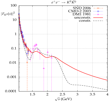
Figure 1: The experimental data [25, 26, 27, 28, 29] compared to the model fits results (see text for details).

Two versions of the model were used, one with an additional assumption $c_{\rho_{n}}=c_{\omega_{n}}$ (the ’constrained’ model) and one without this assumption (the ’unconstrained’ model). $N_{\phi}$, $N_{\omega}$, $N_{\rho}$ indicate the highest radial resonance used in the fit. For the resonances above these values their model parameters were used. $N_{\phi}=2$, $N_{\rho}=3$ for the constrained model and $N_{\phi}=1$, $N_{\rho}=2$, $N_{\omega}=2$ for the unconstrained model. The unconstrained model fits the data better [17], but the quality of the second fit is also reasonable. It is interesting to observe that the models give distinct predictions in the region were there are no data available (Fig. 1), even if in the region were data are available their behaviour is very similar.

It is also of interest to see how much important is the infinite tower of the resonances in the form factors. In Fig. 2 the relative difference of the form factors without (’no tail’) and with the infinite tower of resonances is shown. In the latter case only $N_{i}+1\ ,\ i=\phi,\omega,\rho$ resonance contributions are included. As one could guess, the contributions of the higher resonances to the form factors are more pronounced for higher invariant masses, but they are not negligible even in the lower invariant mass range, where the fitted resonances are situated. A similar behaviour of the pion form factor was observed in [17].

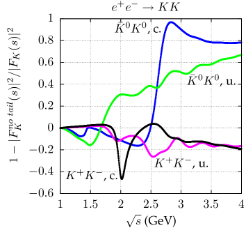
Figure 2: Comparison of the kaon form factors with and without (’no tail’) infinite tower of resonances. c. denotes the constrained model, u. the unconstrained one.

3 Description of narrow resonances

The narrow resonance (only $J/\psi$, $\psi(2S)$ and $\phi$ were considered) contributions were included [17] into the Monte Carlo generator PHOKHARA for the muon, the charged pion and the kaon (both charged and neutral) pair production through the following substitution $\frac{1}{1-\Delta\alpha(s)}\to C^{VP}_{R,P}(s)\ ,\ P=\mu,\pi,K^{+},K^{0}\ ,\ R=J/\psi,\psi(2S)$ , where

$$C^{VP}_{R,P}(s) = \frac{1}{1-\Delta\alpha(s)}-\frac{3\Gamma_{e}^{\phi}}{\alpha m_{\phi}}\ BW_{\phi}(s)\delta_{P}$$ (4)

$$+C_{J/\psi,P}(s)+C_{\psi(2S),P}(s)\ ,$$

$$C_{R,P}(s)=\frac{3\sqrt{s}}{\alpha}\frac{\Gamma_{e}^{R}(1+c_{P}^{R})}{s-M_{R}^{2}+i\Gamma_{R}M_{R}}\ .$$ (5)

For $P=\mu$ and $P=\pi$, $c_{P}^{R}=0$ (it was assumed that the narrow resonances do not decay directly into $\mu^{+}\mu^{-}$ and $\pi^{+}\pi^{-}$). The $\phi$ contributions to the kaon pair production are included in the kaon form factor, hence $\delta_{K}=0$, while $\delta_{P}=1$ for $P=\mu$ and $P=\pi$. The notation and the detailed description of the narrow resonance contribution to the amplitude can be found in [19] together with numerical values of the $c_{P}^{R}$ couplings.

4 PHOKHARA 7.0

The new form factors described in Section 2 and the couplings of $\mu^{+}\mu^{-}$, $\pi^{+}\pi^{-}$, $K^{+}K^{-}$ and $\bar{K}^{0}K^{0}$ pairs to narrow resonances described shortly in Section 3 were implemented into a Monte Carlo event generator PHOKHARA. It’s new release (PHOKHARA 7.0) contains also the implementation of the 4-pion hadronic currents as described in [16], not included in the previous releases of the code. The code can be found on the web page http://ific.uv.es/~ rodrigo/phokhara/ , where also a user guide is provided.

The variance reduction through standard change of variables using the Breit-Wigner shape of resonances was enough to allow for a reasonable acceptance rate. Other technical problems with the treatment of the narrow resonances and their solution were discussed at length in [17, 30] and will not be repeated here.

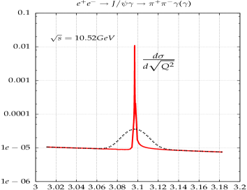
Figure 3: A comparison of the $\pi^{+}\pi^{-}$ ’true’ (solid line) invariant mass spectra and the $\pi^{+}\pi^{-}$ invariant mass spectra seen in a detector with a resolution of 14.5 MeV ( as for the BaBar detector [31]) - dotted line.

A typical invariant mass spectrum of the final meson or muon pair in the vicinity of a narrow resonance, as seen in a radiative return experiment, resembles more a resolution curve of a detector then the shape of the resonance. A typical picture is shown in Fig. 3, where the generated mass spectrum of the $\pi^{+}\pi^{-}$ pair was convoluted with a Gaussian with a detector resolution of the BaBar detector [31].

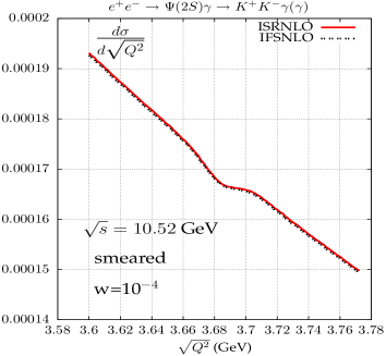
Figure 4: The $K^{+}K^{-}$ invariant mass spectra seen in a detector with a resolution of 14.5 MeV ( as for BaBar detector [31]) including only ISR NLO corrections (ISRNLO) and adding also FSR NLO corrections (FSRNLO).

For the $\psi(2S)$ resonance the smearing effects to large extend dilute the influence of the resonance on the invariant mass spectrum, as shown in Fig. 4 for the charged kaon pair invariant mass distribution. Thus to study it with the radiative return method fairly large statistics is required and it is difficult to expect that the method can compete with the accuracy of scan experiments.

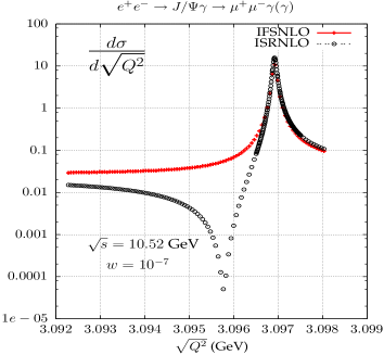
Figure 5: Comparisons of the muon pair invariant mass distributions taking into account only ISRNLO contributions and the complete (ISR+FSR)NLO result.

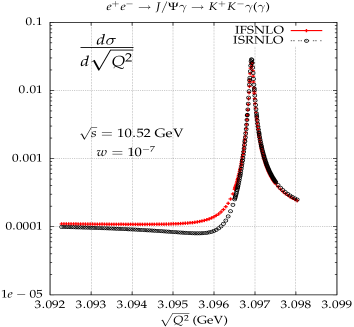
Figure 6: Comparisons of the charged kaon pair invariant mass distributions taking into account only ISRNLO contributions and the complete (ISR+FSR)NLO result.

The contributions from the $J/\psi$ to all studied invariant mass spectra is sizable and one can study the $J/\psi$ decays with a good accuracy. Thus a legitimate question is how big are the contributions coming from the final state photon radiation (FSR). If the detector smearing effects are not taken into account, the distortions of the meson (muon) pair invariant mass distribution by the FSR effects, as compared to ISR, are huge as shown in Figs. 5 and 6. They are still sizable when one takes into account the smearing effects, as evident from Figs. 7 and 8. Moreover they do depend on the event selection [30]. However in the integrated cross section to large extend the corrections cancel. For the muon pair production $\sigma_{ISRNLO}=6.901$ pb and $\sigma_{IFSRNLO}=6.954$ pb, while for the charged kaon pair production $\sigma_{ISRNLO}=2.450\cdot 10^{-5}$ nb and $\sigma_{IFSNLO}=2.442\cdot 10^{-5}$ nb. Thus when one uses only the integrated spectra the FSR corrections can be safely neglected.

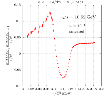
Figure 7: The relative ratio of the muon pair invariant mass distributions taking into account only ISRNLO contributions and the complete (ISR+FSR)NLO result. Detector smearing effects are taken into account.

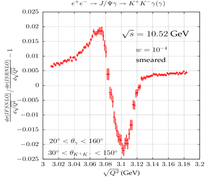
Figure 8: The relative ratio of the charged kaon pair invariant mass distributions taking into account only ISRNLO contributions and the complete (ISR+FSR)NLO result. Detector smearing effects are taken into account.

5 Summary

The implementation into the PHOKHARA Monte Carlo event generator of the narrow resonance contributions is presented and the possibility of studies of the narrow resonances at B factories is discussed.

References

- [1] Andreas Hoecker, these proceedings
- [2] Thomas Teubner, these proceedings
- [3] Min-Shih Chen and P. M. Zerwas, Phys. Rev. D 11 (1975) 58.
- [4] S. Binner, J. H. Kühn and K. Melnikov, Phys. Lett. B 459 (1999) 279 [hep-ph/9902399].
- [5] H. Czyż and J. H. Kühn, Eur. Phys. J. C 18 (2001) 497 [hep-ph/0008262].
- [6] G. Rodrigo, A. Gehrmann-De Ridder, M. Guilleaume and J. H. Kühn, Eur. Phys. J. C 22 (2001) 81 [hep-ph/0106132].
- [7] J. H. Kühn and G. Rodrigo, Eur. Phys. J. C 25 (2002) 215 [hep-ph/0204283].
- [8] G. Rodrigo, H. Czyż, J.H. Kühn and M. Szopa, Eur. Phys. J. C 24 (2002) 71 [hep-ph/0112184].
- [9] H. Czyż, A. Grzelińska, J. H. Kühn and G. Rodrigo, Eur. Phys. J. C 27 (2003) 563 [hep-ph/0212225].
- [10] H. Czyż, A. Grzelińska, J. H. Kühn and G. Rodrigo, Eur. Phys. J. C 33 (2004) 333 [hep-ph/0308312].
- [11] H. Czyż, J. H. Kühn, E. Nowak and G. Rodrigo, Eur. Phys. J. C 35 (2004) 527 [hep-ph/0403062].
- [12] H. Czyż, A. Grzelińska, J. H. Kühn and G. Rodrigo, Eur. Phys. J. C 39 (2005) 411 [hep-ph/0404078].
- [13] H. Czyż, A. Grzelińska and J. H. Kühn, Phys. Lett. B 611 (2005) 116 [hep-ph/0412239].
- [14] H. Czyż, A. Grzelińska, J. H. Kühn and G. Rodrigo, Eur. Phys. J. C 47 (2006) 617 [arXiv:hep-ph/0512180].
- [15] H. Czyż, A. Grzelińska and J. H. Kühn, Phys. Rev. D 75, 074026 (2007) [arXiv:hep-ph/0702122].
- [16] H. Czyż, J. H. Kühn and A. Wapienik, Phys. Rev. D 77, 114005 (2008) [arXiv:0804.0359 [hep-ph]].
- [17] H. Czyż, A. Grzelińska and J. H. Kühn, Phys. Rev. D 81 (2010) 094014 [arXiv:1002.0279 [hep-ph]].
- [18] S. Actis et al., arXiv:0912.0749 [hep-ph].
- [19] H. Czyż and J. H. Kühn, Phys. Rev. D 80 (2009) 034035 [arXiv:0904.0515 [hep-ph]].
- [20] C. Bruch, A. Khodjamirian and J.H. Kühn, Eur. Phys. J. C 39 (2005) 41, [hep-ph/0409080].
- [21] T. K. Pedlar et al. [CLEO Collaboration], Phys. Rev. Lett. 95, 261803 (2005) [arXiv:hep-ex/0510005].
- [22] J. Milana, S. Nussinov and M. G. Olsson, Phys. Rev. Lett. 71, 2533 (1993) [arXiv:hep-ph/9307233].
- [23] C. A. Dominguez, Phys. Lett. B 512, 331 (2001) [arXiv:hep-ph/0102190].
- [24] K. Nakamura et al. [ Particle Data Group Collaboration ], J. Phys. G G37 (2010) 075021.
- [25] F. Mane, D. Bisello, J. C. Bizot, J. Buon, A. Cordier and B. Delcourt, Phys. Lett. B 99, 261 (1981).
- [26] M. N. Achasov et al., Phys. Rev. D 63, 072002 (2001).
- [27] R. R. Akhmetshin et al., Phys. Lett. B 551, 27 (2003) [arXiv:hep-ex/0211004].
- [28] R. R. Akhmetshin et al. [CMD-2 Collaboration], Phys. Lett. B 578, 285 (2004) [arXiv:hep-ex/0308008].
- [29] M. N. Achasov et al., J. Exp. Theor. Phys. 103, 720 (2006) [Zh. Eksp. Teor. Fiz. 103, 831 (2006)] [arXiv:hep-ex/0606057].
- [30] H. Czyż and A. Grzelińska, Chinese Physics C 34 (2010) 855.
- [31] B. Aubert et al. [BABAR Collaboration], Phys. Rev. D 69 (2004) 011103 [arXiv:hep-ex/0310027].