Hydrodynamics of Hypersonic Jets: Experiments and Numerical Simulations

Abstract

Stars form in regions of the galaxy that are denser and cooler than the mean interstellar medium. These regions are called Giant Molecular Clouds. At the beginning of their life, up to $10^{5}-10^{6}$ years, stars accrete matter from their rich surrounding environment and are origin of a peculiar phenomenon that is the jet emission. Jets from Young Stellar Objects (YSOs) are intensively studied by the astrophysical community by observations at different wavelengths, analytical and numerical modeling and laboratory experiments. Indications about the jet propagation and its resulting morphologies are here obtained by means of a combined study of hypersonic jets carried out both in the laboratory and by numerical simulations.

1 Introduction

The physical parameters of astrophysical jets are impossible to reproduce in any Earth’s laboratory. We therefore must limit ourselves to identify those parameters that are the crucial ones in controlling the overall jet behavior and to rescale the laboratory simulations accordingly. Among the many parameters that describe the jet evolution and propagation features, two of them are paramount: the Mach number and the jet to ambient density ratio (Ferrari, 1998; Reipurth and Bally, 2001). We have therefore devised an experiment where these two parameters can be set to match the ones derived from observations of YSO jets (Belan et al., 2004).

In order to better understand the dynamical details of the jet propagation and evolution, we have carried out 3D numerical hydrodynamic simulations adopting boundary and injection conditions that were as close as possible to the experimental ones. The numerical results show good agreement with the laboratory data, namely: the jet head velocity is consistent for the two situations, the presence of bright knots along the jet is correctly reproduced, and non-axisymmetric perturbations, seen in the heavy jet case, rise and grow in the simulation to resemble the laboratory jet.

Observations show that stellar jets extend in space for very long distances, in fact they can reach lengths of hundreds, even thousands, jet radii. While the initial collimation, at the launching region, is likely to be magnetic, however at very large distances from the origin stellar jets maintain their small free-jet opening angle, consistently with a Mach number ranging between 10 and 40. Here we show that laboratory hydro hypersonic jets maintain their structure, at least up to 70 jet radii.

The plan of the paper is the following: in Section 2 and 3 we present the apparatus setup and the numerical code, Section 4 is dedicated to the comparison of experimental and numerical results, and the conclusions are drawn in Section 5.

2 Experimental setup

The jets under study are created inside a modular vacuum vessel, with a maximum length of 5m and a diameter of 0.5m. Several kinds of nozzles can be mounted on this vessel. The vessel diameter is much larger than the diameter of the jets, so that the lateral walls effects are limited. The required ambient inside the vessel is obtained by means of a system of valves which sets the desired ambient density (at pressures in the 1.5 to 100 Pa range) using a gas in general different from the jet gas. An electron gun operating at very low pressures, thanks to a set of secondary pumps, and equipped with a deflection system, creates an electron sheet. This sheet intercepts the jet under test, and generates a plane fluorescent section of the flow. These fluorescent zones can be acquired by different kinds of cameras, including intensified devices, depending on the experiment to be performed. The cameras and the electron gun can be mounted on different ports. The vessel including all the available sections is shown in fig. 1.

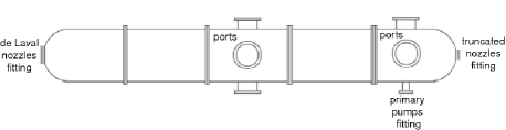
Fig. 1 : Sketch of the vacuum vessel including all the available sections. The ports can be used for camera or electron gun mounting. Ambient gas valve fittings and electrical/service connectors are not shown.

This system was already employed to study the properties of highly underexpanded jets, making use of truncated nozzles and color CCD cameras, detailed information can be found in the previous works by Belan et al. (2004, 2006); Belan, De Ponte and Tordella (2008).

In the present setup, by means of a fast piston, the jet gas is compressed to stagnation pressures in the 0.1 to 0.7 MPa range, then it is accelerated by a de Laval nozzle and enters the vacuum vessel, mounted in the 3-modules configuration. The jet parameters attainable by the experimental system are outlined in table 1.

The nozzle used in this experiment has been carefully designed to perform nearly isoentropical gas accelerations and expansions, i.e. flows as close as possible to the ideal conditions, but accounting for friction and heat exchange effects.

The nozzles were built at the CERN workshop of Geneva with surface accuracies in the order of 1$\mu$m. Under such conditions, the flow at the nozzle outlet has the design Mach number over a very wide cross-section, excluding a thin boundary layer region at the walls, provided that the stagnation-to-ambient pressure ratio $p_{0}/p_{a}$ maintained between inlet and outlet has a well defined value. In this experiment, the stagnation-to-ambient pressure ratio $p_{0}/p_{a}$ is checked by means of high accuracy pressure transducers. The Mach number is then obtained by a numerical method that takes into account the effects of the boundary layer and heat exchange with the nozzle walls. However the result differs by the well-known steady-state ideal relationship:

$$M^{2}=\frac{2}{\gamma-1}\left[\left(\frac{p_{0}}{p_{a}}\right)^{\frac{\gamma-1}{\gamma}}-1\right]$$

by about 1%.

Table 1 : Jets parameters in the present experiment

Nozzle geometry	De Laval
Stagnation/ambient pr. ratio $p_{0}/p_{\rm amb}$	300 to $2\cdot 10^{5}$
Mach number $M_{max}$	5 to 20
Density ratio $\rho_{\rm jet}/\rho_{\rm amb}$	0.01 to 110
Reynolds, throat diameter based $Re_{n}$	$10^{4}$ to $5\cdot 10^{4}$
Reynolds, jet diameter based $Re_{D}$	up to $2\cdot 10^{6}$
Reynolds, axial length based $Re_{x}$	$>10^{7}$

Several nozzles in the Mach number range $5\leq M\leq 20$ are available, in this experiment a nozzle designed to generate a $M$ = 15 at the exit has been used. The nozzle exit diameter is $2r_{0}=0.07136$ m. Slightly different Mach numbers can be obtained by adjusting the stagnation/ambient pressure ratio $p_{0}/p_{a}$ around the ideal isoentropic value $4.76\cdot 10^{4}$. The present setup is sketched in fig. 2, where the vessel has a length of 2.46 m, and the camera (optical) window is 0.27 m wide.

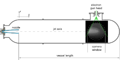
Fig. 2 : Typical setup for matched jets at M=15

In each run a pair of gases is selected for the jet and the ambient. The available gases are helium, argon, xenon and air, only the first three ones are used for the jet since the nozzle is designed for monoatomic gases. The jets meet the electron sheet under the optical window, and the resulting images are acquired by an intensified CMOS camera; besides visualizations, density and structure velocities measurements are possible by image-processing.

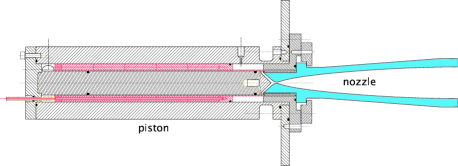
Fig. 3 : Longitudinal section of the piston-nozzle system. The piston is shown at the starting position

The physical time scale of jets $\tau$ can be defined as the ratio between the jet radius at the nozzle exit $r_{0}$ and the speed of sound internal to the jet under nominal conditions, i.e. when the nozzle works under ideal steady conditions, and is in the order of 0.1 to few ms. In the following, we will express time in units of $\tau$ and lengths in units of $r_{0}$.

The piston-nozzle system is shown in fig. 3. The jet gas is compressed in a chamber that leads to the nozzle inlet. At the end of the compression run, owing to the valves opening, the outflow increases to a maximum value, then it diminishes as the gas contained in the chamber is used up. The mass flow $Q$ is a function of time of the kind

$$Q=Q[p_{0}(t),f(t),g(t)],$$

where $p_{0}$ is the pressure in the piston chamber, $f(t)$ is a factor function which accounts for the progressive opening of the valves, and $g(t)$ is the function which accounts for the natural decay in the amount of gas remaining in the compression chamber after the piston stop. This model, which is based on the piston-valve behavior, gives the following for density, pressure and velocity of the gas at the nozzle exit:

$$\rho_{\rm jet}\sim Q(t)^{2/3},\;p_{\rm jet}\sim Q(t)^{2/3}/\gamma,v_{\rm jet}\sim{M}\ Q(t)^{1/3},$$

where $M$ is the Mach number at the end of the nozzle. The resulting gas injection curve has the shape sketched in fig. 4. In this experiment two jets are considered, a light He jet flowing in a Xe ambient and a heavy Xe jet flowing in an air ambient.

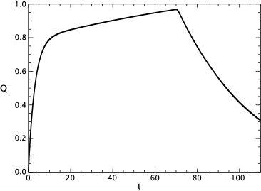
Fig. 4 : A typical jet gas injection: dimensionless nozzle mass flow versus dimensionless time. The mass flow $Q$ is normalized over the reference flow rate $Q_{r}$ which is yielded by the same nozzle when operating in ideal steady conditions. For the Helium jet, $Q_{r}$ is $0.43$ g/s and for the Xenon jet, $Q_{r}$ is $2.44$ g/s. Time is normalized over the jet time unit $\tau$ (ratio between the jet radius at the nozzle exit and the speed of sound internal to the jet). The piston output valves begin to open at $t=0$. In general, the jet hits the vessel end during the increasing phase of $Q(t)$

3 The numerical code PLUTO

The numerical code was developed for the solution of hypersonic flows in 1, 2, and 3 spatial dimensions and different systems of coordinates (Mignone et al., 2007; Mignone, 2009). The code provides a multiphysics, multialgorithm modular environment particularly oriented toward the treatment of astrophysical flows in presence of discontinuities. Different hydrodynamic modules and algorithms may be independently selected to properly describe Newtonian, relativistic, MHD, or relativistic MHD fluids.

The modular structure exploits a general framework for integrating a system of conservation laws, built on modern Godunov-type shock-capturing schemes. The discretization recipe involves three general steps: a piecewise polynomial reconstruction followed by the solution of Riemann problems at zone interfaces and a final evolution stage.

4 Results

4.1 Experiments/numerical simulations comparisons

A slightly underdense (light) jet, Mach 15, density ratio 0.7 is shown in fig. 5.

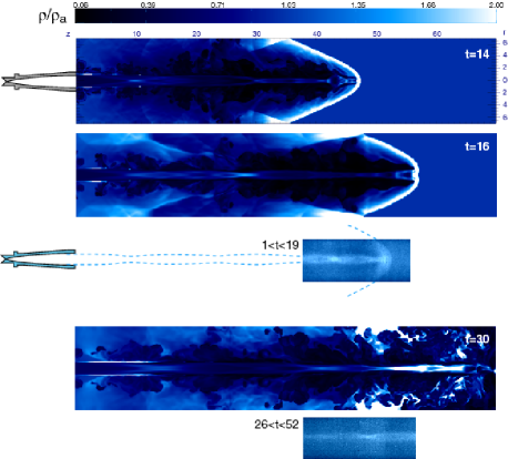
Fig. 5 : Light jet, Helium in Xenon. $M$=16.1, ambient pressure $p_{a}=4.0\pm 0.1$Pa, estimated nozzle exit velocity = 3200 $\pm$330 m/s, mean jet pressure at nozzle exit $p_{j}=p_{a}\pm 30$%, stagnation/ambient pressure ratio $p_{0}/p_{a}=7\cdot 10^{4}\pm 30$%. Comparison of numerical simulations (density maps) and visualizations (superpositions of scaled correlated frames). The density maps are normalized to the unperturbed ambient value. The space unit is the exit radius of the nozzle $r_{0}=0.03568$ m. The time unit for this light jet is $\tau=0.18$ ms

In this jet, dense knots form spontaneously on the axis well before the impact to the vessel end. They are visible both in the numerical and in the experimental images. After the impact, the interaction with the reflected flow does not spoil the axial symmetry of the flow. The impact of this jet on the vessel end wall reflects only a very small amount of matter, hence the perturbation may be considered weak. It is also noticeable that the inner part of the flow remains compact and collimated after the impact. This is also an interesting information, which could open the way to other applications, in particular to perturbative near-linear experimental studies. The inertial effects, and the associated compressibility, must here be so powerful to inhibit the spatial growth of the jet, unlike what happens in the incompressible situation, where sheared flows generally grow fast in thickness.

An overdense (heavy) jet, Mach 15, density ratio 100, is shown in fig. 6

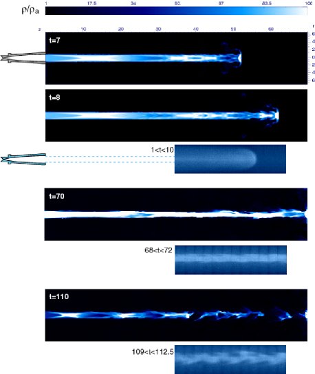
Fig. 6 : Heavy jet, Xenon in Air. $M$=15, ambient pressure $p_{a}=9.95\pm 0.1$ Pa, estimated nozzle velocity at the exit = 560 $\pm$ 60m/s, mean jet pressure at the nozzle exit $p_{j}=p_{a}\pm 30$%, stagnation/ambient pressure ratio $p_{0}/p_{a}=4.76\cdot 10^{4}\pm 30$%. Comparison of numerical simulations (density maps) and visualizations (superpositions of scaled correlated frames). The density maps are normalized to the unperturbed ambient value. The space unit is the exit radius of the nozzle $r_{0}=0.03568$ m. The time unit for this heavy jet is $\tau=0.96$ ms

Here, there are overdense zones on the axis, they are very close to each other, and are resolved only in the numerical simulation. For the heavy jet, the interaction with the reflected flow eventually produces a finite perturbation, which non linearly interacts with the outflow. This is sufficient to spoil the axial symmetry. However, it is not sufficient to spoil the collimation of the jet. This suggests the possibility of a very large longitudinal extent of the heavy hypersonic jet and its related capability to transfer energy, momentum and mass to large distances (on the Earth, in space, in possible new applications).

An example of hypersonic jet with a completely different behaviour is reported in fig. 7, where an underdense jet having Mach number and density ratio similar to the ones of the jet in fig. 5 is shown (Belan, De Ponte and Tordella (2008, 2010)). In this case, the jet is created by means of a truncated nozzle, and is far from being nearly isoentropic. It is in fact characterized by a strong normal shock close to the nozzle exit, and by a lateral spreading which in the long term is remarkably larger than that in fig. 5. The reduction of the core diameter is clear (the jet head is outside the image on the right) and is also a measure of the spreading of the annular mixing layer that surrounds it. The mixing region is slow compared to the flow in the core and is not visible in this figure. However, it can be observed through concentration measurements (Belan, De Ponte and Tordella (2008, 2010)). In this example the spreading angle with respect to the jet axis is about 8 degrees (Belan, De Ponte and Tordella (2010)).

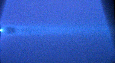
Fig. 7 : Helium jet in an Argon medium: highly underexpanded jet, maximum Mach number = 16, stagnation/ambient pressure ratio $p_{0}/p_{a}=304$, density ratio after the normal shock $\sim 0.15$.

4.2 Results analysis

The velocities of flow structures (jet’s head, knots, traveling waves..) can be measured by means of standard correlation techniques applied to the pixel matrices of consecutive images.

For the light jet of fig. (5), in the simulations the head (bow shock) velocity grows from $440\pm 3$m/s to $706\pm 3$m/s in the $2<t<16$ time interval (before the impact to the vessel end) due to the increase in the mass flow. The experimental head velocity at $t=15$ measured by image correlation is $490\pm 140$m/s. For the heavy jet of fig. (6), the jet head velocity grows from $130\pm 3$m/s to $270\pm 3$m/s in the $2<t<9$ time interval, and the experimental value at $t=8$ is $140\pm 30$m/s.

When the velocity of a structure is known, two images in succession containing the same structure can also be superimposed after shifting the second one by the displacement of the structure under study. Then, this procedure can be repeated, and a spatial reconstruction of a part of the jet structure larger than the camera window can be done by superimposing parts of adjacent frames (’slices’). Clearly, the reconstruction of jet morphology on large scales has a physical meaning only if the changes in structure properties are slow with respect to the interframe time.

Two image reconstructions for a light jet and a heavy jet, obtained by correlated frames superposition, are shown in figures 8 and 9. These figures are constructed overcoming the validity range of the technique in order to obtain single pictures visualizing a whole jet or a large part of it, the resulting images must be considered as ’frozen’, as if the jet were passing through the camera window without changes in its morphology.

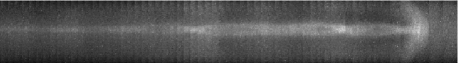
Fig. 8 : ’Frozen’ image of the light jet analyzed in figure 5, Helium in Xenon at $M$=16.1, obtained by superimposed frames in the time range $0<t<66\tau$

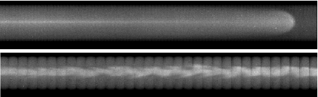
Fig. 9 : ’Frozen’ images of a heavy jet, Xe in Ar at $M$=13.5, obtained by superimposed frames in the time ranges $0<t<20\tau$ and $60\tau<t<70\tau$

The effect of the lateral boundaries of the vessel can be estimated by changing the boundary conditions in the numerical simulations. Figure 10 compares longitudinal 2D cuts, at $t=14$, of the light jet simulation obtained employing the actual lateral boundary conditions with the one obtained with outflow conditions, Differences in the density distribution morphologies are visible at the jet’s head, that appears slightly narrower in the free-boundary simulation, while the head’s positions differ by a few percent in the two cases. The shock reflection at $x\sim 36$ is absent in the free-boundary case.

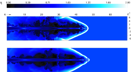
Fig. 10 : Comparison between simulations with and without lateral boundaries at $t=14$

5 Conclusions

Our experiment highlights the following aspects:

I) - the collimation of near-isoentropic jets over distances much larger that the initial radius.

II) - the jet persistence (which, for the light jet, is mantained even after the impact with the vessel end-wall).

III) - the presence of a cocoon surrounding the underdense jet, while this is not visible for the overdense one.

IV) - the spontaneous formation of knots along the jet axis (before the impact of the jet to the vessel end).

These aspects refer both to numerical simulations and to experiments ruled by Newtonian dynamics, and do not need of the confining effect associated to the presence of magnetic fields.

Some of these aspects are common to stellar jets, in particular the jet confinement and persistence over long distances, in units of the initial radius.

References

- Ferrari (1998) Ferrari, A.: ARA&A, 36, 539 (1998)
- Reipurth and Bally (2001) Reipurth, B. and Bally, J., ARA&A, 39, 403 (2001)
- Belan et al. (2004) Belan M., De Ponte S., Massaglia S., Tordella D.: Astrophys. Space Sci., 293 (1-2), 225-232 (2004)
- Belan et al. (2006) Belan M., De Ponte S., Tordella D.: EFMC6 KTH, Euromech Fluid Mechanics Conference 6, Royal Institute of technology, Stockholm (2006)
- Belan, De Ponte and Tordella (2008) Belan M., De Ponte S., Tordella D.: Exp Fluids, 45, 3 (2008)
- Belan, De Ponte and Tordella (2010) Belan M., De Ponte S., Tordella D.: Phys Review E, 82, 2 (2010)
- Mignone et al. (2007) Mignone, A. et al.: ApJS, 170, 228 (2007)
- Mignone (2009) Mignone, A.: Nuovo Cimento della Societa’ Italiana di Fisica C-Colloquia on Physics, 32, 2, 37-40 (2009)