Fixation, transient landscape and diffusion’s dilemma in stochastic evolutionary game dynamics

Abstract

Agent-based stochastic models for finite populations have recently received much attention in the game theory of evolutionary dynamics. Both the ultimate fixation and the pre-fixation transient behavior are important to a full understanding of the dynamics. In this paper, we study the transient dynamics of the well-mixed Moran process through constructing a landscape function. It is shown that the landscape playing a central theoretical “device” that integrates several lines of inquiries: the stable behavior of the replicator dynamics, the long-time fixation, and continuous diffusion approximation associated with asymptotically large population. Several issues relating to the transient dynamics are discussed: 1) Multiple time scales phenomenon associated with intra- and inter-attractoral dynamics; 2) discontinuous transition in stochastically stationary process akin to Maxwell construction in equilibrium statistical physics; and 3) the dilemma diffusion approximation facing as a continuous approximation of the discrete evolutionary dynamics. It is found that rare events with exponentially small probabilities, corresponding to the uphill movements and barrier crossing in the landscape with multiple wells that are made possible by strong nonlinear dynamics, plays an important role in understanding the origin of the complexity in evolutionary, nonlinear biological systems.

I Introduction

One of the salient features of the stochastic evolutionary game dynamics for finite populations is the fixation Nowak book ; Traulsen's review ; Roca09PLR . That is, no matter how the initial strategies are distributed in a population, the system will eventually be fixated to only one strategy. In general, this phenomenon can be theoretically explained in terms of a Markov process with absorbing state(s) Karlin book ; Durrett book : The limiting theory of Markov processes tells us that the finite-state Markov chains with absorbing states will eventually be trapped into one of the absorbing states as time passes. The well-known Wright-Fisher model Fisher1922on ; Wright1931evolution , Moran process Moran book ; Nowak Nature 04 and the pairwise comparison processes Traulsen 07 Fermi ; Fu10JTB all belong to this class. A further classification of Darwinian selection scenarios based on the fixation descriptions has already been established in stochastic game dynamics Taylor BMB 04 ; Antal BMB 06 ; Taylor06JTB ; Ohtsuki JTB 07 ; Altock NTP 09 ; Wubin2010PRE . Another important class consists of evolutionary dynamics with mutations where an ergodic mutation-selection equilibrium can be reached Fudenberg TPB 06 ; Antal09JTBa ; Antal09JTBb . The latter is out of the scope of our study; However, the landscape introduced in the present work provides a unified perspective for both classes of processes.

In addition to the ultimate fixation, attention should also be paid to the time-dependent, pre-fixation transient behavior for several reasons szabo2007evolutionary ; DrozEPJ ; SzaboPRE : On one hand, the process to fixation is intimately dependent upon both the transient movements before absorption and the one last step to fixation. That is, studying the transient dynamics provides important insights into the final fixation behavior. On the other hand, sometimes the time for a true fixation is too long to be observed Antal BMB 06 and the relevant time scale can be shorter Huisman Nature 99 ; Huisman Ecology 01 ; Dorroch 1965 . In this case, the transient dynamics provides a more appropriate description. Furthermore, examinations of transients can yield a mechanistic understanding of the persistence and coexistence in complex biological dynamics, especially in ecosystems Hastings 04 . Indeed, it has been found that the pre-fixation transient dynamics could be an essential explanatory aspect of characterizing the stochastic fluctuations raised from finite populations Block BMB 2000 ; Claussen 05 PRE ; Tao BMB 07 ; Vellela BMB 07 ; Ficici JTB 07 .

The theory of quasi-stationarity is a widely applied, standard technique of studying the pre-fixation process quasibook . It defines the subchain with the absorbing states removed. Based on this approach, we present an extended analysis for the transient dynamics of the well-mixed frequency-dependent Moran process. An ergodic conditional stationary distribution is used to characterize the pre-fixation process. As a result of the law of large numbers, this stationary distribution approaches to a singular distribution in the infinite population limit. The corresponding large deviation rate function Freidlin ; Dembo ; Touchette 10 PR , which is population-size independent, is shown to be a landscape. This transient landscape has a Lyapunov property with respect to the corresponding deterministic replicator dynamics, providing a potential-like function for visualizing the transient stochastic dynamics. Ideas related to the transient landscape of Moran process have been discussed in the past: Claussen and Traulsen Claussen 05 PRE studied non-Gaussian stochastic fluctuations based on the conditional stationary distribution. It is also a general feeling that one can use the negative logarithm of the stationary, or conditional stationary distribution as the potential in evolutionary dynamics, following an analogue to Boltzmann’s law in statistical mechanics. However, it is important to point out that a stationary distribution usually collapses to singular supports in the infinite population limit, while our large deviation rate function $\psi(x)$ is supported on the whole space and it is independent of system’s size. Therefore, in terms of the analogue to Boltzmann’s law, we are effectively identifying the system’s size as the inversed temperature which tends to infinity for a deterministic limit.

Even though our analysis is based on the one-dimensional Moran process, this idea is general. It can be applied to many other multi-dimensional evolutionary game dynamics with finite populations, with or without detailed balance qian_2011_nonlinearity_review . For the latter case, the landscape itself is an emergent property of the dynamics. With respect to Moran process, Roca09PLR ; Antal BMB 06 also discovered the expression of $\psi(x)$ from a different origin, via their approximated calculation of fixation probability for large population size. We shall show that this connection is a nice mathematical property of the $\psi(x)$ function for the processes in one-dimensional case, but its generalization to multi-dimensional cases is not obvious. More specifically, for multi-dimensional systems with multiple alleles, the fixation probability does not naturally give a landscape. The large deviation rate function, however, can be generalized to multi-dimensional Markov processes, as indicated by the Freidlin-Wentzell theory Freidlin . The landscape we introduced is also consistent with the landscape theory for other population dynamics, e.g., chemical, that is ergodic without fixation Wang08PNAS ; qian_2011_nonlinearity_review .

There are two fundamentally different types of movements in this landscape that require separated attention. ($i$) “Downhill movements” which have deterministic counterparts: The local minima (transient attractors) in this landscape correspond to the stable points in the replicator dynamics Taylor and Jonker1978 . That is, these transient attractors are in direct agreement with the evolutionarily stable strategies (ESSs) Maynard book ; Zhou Da JTB 10 . ($ii$) “Uphill movements” which are rare and without a deterministic correspondence. In general, rare events take exponentially long time; one needs to take multiple time scales into consideration in understanding the appropriate fluctuation descriptions for the transient dynamics as well as eventual fixation. This is particularly relevant in the anti-coordination games.

Furthermore, the concept of stochastic bistability is studied in the coordination games. In this case, the downhill and uphill movements in the landscape dominate “intra-attractoral” and “inter-attractoral” dynamics respectively qian_2011_nonlinearity_review . It is shown that a Maxwell-type construction from classic phase transition theory in statistical physics ge hao PRL 09 is necessary as the population size tends to infinity, i.e., only one of attractors should be singled out in such a construction — It corresponds to the global minimum of the landscape. This is not present in the bistable deterministic dynamics; it raises the novel issue of ultimate fixation. It did not escape our notice that it is the exponentially long-time search that ultimately finds the global minimum in a “non-convex optimization” non convex .

Another important issue directly relating to the transient dynamics is the diffusion approximation Feller1954diffusion ; Gardiner book ; tan2000stochastic . With the conventional truncation of Kramers-Moyal (KM) expansion, the discrete stochastic Moran process for large populations has been approximated by a stochastic differential equation Traulsen PRL05 ; Chalub 08 , with absorbing Dirichlet boundary conditions. If one replaces the absorbing boundary conditions with the reflecting ones, we can also derive an ergodic stationary distribution from the Fokker-Planck equation of this diffusion process. It will be shown that this stationary distribution is in fact the “conditional” stationary distribution for the process with absorbing boundary conditions. In a comparison of the transient dynamics between the original Moran process and its continuous counterpart, it is shown that even though the KM diffusion is valid in finite time as a local dynamical approximation, it could lead to incorrect approximation in global inter-attractoral dynamics. In bistable game systems, particularly, the KM diffusion could single out a different stable point from that of the original process for large but finite populations. Moreover, enlightened by Hänggi et al.’s work hanggi1984bistable , we also consider their diffusion approximation that provides the correct global dynamics. However, this diffusion process gives incorrect finite time stochastic dynamics.

Now we have a diffusion’s dilemma: The truncated KM diffusion gives the correct finite time stochastic dynamics as the original Moran process with large population size (this is guaranteed both by the so called van Kampen’s system size expansion van Kampen and Kurtz’s theorem Kurtz1976 ; Kurtz1978 ), but wrong stationary distribution. On the other hand, Hänggi et al.’s diffusion, which is unique in providing the correct stationary distribution as well as deterministic limit, is wrong for the finite time stochastic dynamics. To further illustrate this diffusion’s dilemma, a simple example is present. By investigating the first passage times, it is found that the failure of exponential approximation in the uphill movement could be the origin of the difficulties of diffusion approximation. In other words, diffusion approximation is a second-order polynomial expansion for the Kolmogorov forward equation of the original discrete process, which can give the correct Gaussian dynamics near the stable point; However, the inter-attractoral global dynamics, determined by the barrier crossing events with exponential small probabilities, should be approximated in the level of exponential asymptotics.

This paper is organized as follows: In Sec. II, we introduce the frequency-dependent Moran process. Then we give the transient description of the Moran process in Sec. III, where the transient landscape $\psi(x)$ is constructed. It is shown that this landscape as a “glue” holds the deterministic replicator dynamics, the fixation and the problem of Maxwell-type construction together. Diffusion’s dilemma is discussed in Sec. IV. The discussions are included in the last section.

II Frequency-dependent Moran process

To study evolutionary game theory in finite populations, Nowak et al. Nowak Nature 04 generalized Moran’s classical population genetic model Moran book by using frequency-dependent fitness. Consider a population of $N$ individuals playing a symmetric $2\times 2$ game with strategies $A$ and $B$, the payoff matrix is

$$M=\left(\begin{array}[]{cc}a&b\\ c&d\end{array}\right),$$ (1)

where all the entries in the matrix are assumed to be non-negative. If $i$ players follow strategy $A$, and $N-i$ play $B$, the the average payoff of an individual of $A$ is

$$F_{A}^{i}=\frac{a(i-1)+b(N-i)}{N-1},$$ (2)

where self-interaction is excluded, and also for $B$ is

$$F_{B}^{i}=\frac{ci+d(N-i-1)}{N-1}.$$ (3)

Fitness is assumed to be a linear combination of background fitness and the payoff as follows:

$$f_{A}^{i}=1-w+wF_{A}^{i},$$ (4)

$$f_{B}^{i}=1-w+wF_{B}^{i},$$ (5)

where $w\in[0,1]$ denotes the intensity of selection.

At each time step, one individual is chosen to reproduce proportional to its fitness, then the offspring replaces a randomly chosen individual, so that the population size is constant. The evolutionary mechanism in this Moran process, thus, can be conveniently described as a Markov chain. If we denote $X$ as the the number of individuals following strategy $A$, then $X$ is actually a finite-state birth-death process with discrete-time steps, which can be expressed as follows:

$$0\overset{T_{1}^{-}}{\longleftarrow}1\underset{T_{2}^{-}}{\overset{T_{1}^{+}}{\rightleftharpoonsfill{20pt}}}2\rightleftharpoonsfill{20pt}\cdot\cdot\cdot\rightleftharpoonsfill{20pt}(N-2)\underset{T_{N-1}^{-}}{\overset{T_{N-2}^{+}}{\rightleftharpoonsfill{20pt}}}(N-1)\overset{T_{N-1}^{+}}{\longrightarrow}N,$$

where the birth and death probabilities conditional on the present state $X=i$ are

$$T_{i}^{+}=P(i\rightarrow i+1)=\frac{if_{A}^{i}}{if_{A}^{i}+(N-i)f_{B}^{i}}\frac{N-i}{N},$$ (6)

$$T_{i}^{-}=P(i\rightarrow i-1)=\frac{(N-i)f_{B}^{i}}{if_{A}^{i}+(N-i)f_{B}^{i}}\frac{i}{N},$$ (7)

$$T_{i}^{0}=P(i\rightarrow i)=1-T_{i}^{+}-T_{i}^{-}.$$ (8)

So the Markov transition probability matrix of this process can be denoted as

$$Q=\left(\begin{array}[]{ccccc}1&0&0&\cdots&0\\ T_{1}^{-}&1-(T_{1}^{+}+T_{1}^{-})&T_{1}^{+}&\cdots&0\\ \vdots&\vdots&\vdots&\vdots&\vdots\\ 0&\cdots&T_{N-1}^{-}&1-(T_{N-1}^{+}+T_{N-1}^{-})&T_{N-1}^{+}\\ 0&\cdots&0&0&1\\ \end{array}\right).$$ (9)

It is easy to see that $X=0$ and $N$ are two absorbing boundaries for the system, so the limiting distribution of the Moran process can be denoted as

$$(1-\rho_{i})\delta_{0}+\rho_{i}\delta_{N},$$ (10)

where $\rho_{i}$ is the fixation probability that $i$ individuals of strategy $A$ succeed in taking over the entire population, and $\delta_{0}$ (or $\delta_{N}$) is a Dirac mass at $0$ (or $N$). In other words, except for the two pure-strategic absorbing states, all the mixed states are transient. This process is different from an irreducible Markov chain whose ergodic behavior is supported on the whole state space. Thus in the Moran process, it is natural to investigate the conditions for selection to favor successful fixation by calculating the corresponding fixation probabilities Taylor BMB 04 .

III transient analysis

The fixation is intimately dependent upon the transient behavior before absorption. To show this, we shall divide the process to fixation into two parts: One is the irreducible transitions among the transient states before absorption, the other is the last step to fixation. This distinction has a very clear evolutionary meaning: the former is a consequence of “global dynamics” while the latter is a rather local event. It is also worth mentioning that these two scenarios correspond so-called “golf-course search” and “funnel perspective” in the field of protein folding Qian02PS . By explicitly studying these two different problems, one is able to address the “dynamic nature of fixation”: Is the dynamics toward fixation inherent in the evolutionary dynamics? The investigation of the transients provides another perspective to understand the fixation. Further, in order to describe the inherent fluctuations arising from finite populations, the transient dynamics has been proved to be an essential explanatory aspect Claussen 05 PRE ; Tao BMB 07 .

III.1 Conditional stationary distribution and the transient landscape

A natural mathematical idea to describe the transient behavior is to concentrate on the distribution conditional on the subspace of the mix-strategic states quasibook . We consider an auxiliary process $X^{*}(t)$ close to the original Moran process $X(t)$. $X^{*}(t)$ can be described as the original process with the absorbing states removed, while all other birth and death probabilities remain unchanged quasibook ; Nasell 99 MB . So the process of $X^{*}(t)$ can be expressed as

$$1\underset{T_{2}^{-}}{\overset{T_{1}^{+}}{\rightleftharpoonsfill{20pt}}}2\rightleftharpoonsfill{20pt}\cdot\cdot\cdot\rightleftharpoonsfill{20pt}(N-2)\underset{T_{N-1}^{-}}{\overset{T_{N-2}^{+}}{\rightleftharpoonsfill{20pt}}}(N-1).$$

Note that $X^{*}(t)$ is an ergodic Markov chain with a unique stationary distribution $\{\eta_{i}\}$, yielding the following iterative relation

$$\eta_{i}=\eta_{1}\prod_{k=2}^{i}\left(\frac{T_{k-1}^{+}}{T_{k}^{-}}\right),~{}~{}~{}~{}i=2,...,N-1.$$ (11)

The interpretation of $\eta$ for the transient description of the original process $X(t)$ is from the theory of quasi-stationarity Dorroch 1965 . It is shown that $\eta$ characterizes the occupation time distribution of the process before absorption, i.e. $\eta_{i}$ is the average times of visiting to $i$ divided by the mean absorbing time (see appendix A). So we call $\eta$ the conditional stationary distribution of the original process.

We write $\eta$ as $\eta^{(N)}$ for its dependence on the population size $N$,

$$\eta^{(N)}_{i}=\eta^{(N)}_{1}\prod_{k=1}^{i}\left(\frac{T_{k-1}^{+}}{T_{k}^{-}}\right)=A\exp\left\{\sum_{k=1}^{i}\ln\left(\frac{T_{k-1}^{+}}{T_{k}^{-}}\right)\right\}.$$

By expanding in the inverse of large population size $N$, $\eta^{(N)}$ can be expressed as

$$\eta^{(N)}(x)=A\exp\left[-N\psi(x)+\psi_{1}(x)+\frac{\psi_{2}(x)}{N}+...\right].~{}~{}~{}x=\frac{i}{N}.$$

where the leading item $\psi(x)$ is the large deviation rate function of $\eta^{(N)}$ Dembo ; Touchette 10 PR ; Ge 10 PRSI . By the Euler-MacLaurin summation formula, we have

$$\psi(x)=-\int_{0}^{x}\ln\left[\frac{T^{+}(y)}{T^{-}(y)}\right]dy,$$ (12)

where

$$T^{+}(y)=\frac{x(1-x)(1-w+w(ax+b(1-x)))}{x(1-w+w(ax+b(1-x)))+(1-x)(1-w+w(cx+d(1-x)))},$$ (13)

$$T^{-}(y)=\frac{x(1-x)(1-w+w(cx+d(1-x)))}{x(1-w+w(ax+b(1-x)))+(1-x)(1-w+w(cx+d(1-x)))}.$$ (14)

We term $\psi(x)$ as the transient landscape, which will be shown to be of great importance in characterizing both deterministic and stochastic dynamics. It should be mentioned that our definition of the transient landscape can be extended to more general dynamics with multiple populations (see appendix B). An relation between $\psi(x)$ and fixation probabilities in Roca09PLR ; Antal BMB 06 will be given in Eq. (16) (Also see appendix D).

For the replicator equation

$$\frac{dx(t)}{dt}=x(1-x)[((a-b)x+b)-((c-d)x+d)],$$

It is easy to check that

$$\dot{\psi}(x(t)) =\frac{d\psi(x)}{dx}\frac{dx}{dt}$$

$$=-\ln\left[\frac{1-w+w((a-b)x+b)}{1-w+w((c-d)x+d)}\right]x(1-x)[((a-b)x+b)-((c-d)x+d)]$$

$$\leq 0.$$

So $\psi(x)$ has the Lyapunov property thompson86book ; Hassan02book , i.e. the dynamical behavior of the replicator dynamics can be predicted by this transient landscape. Note that by our definition of $\psi(x)$, the Lyapunov property is nearly transparent, even for multi-dimensional systems (see appendix B).

We classify the transient landscape into three main generic cases (see Fig. 1):

1) Uni-well: $a<c$ and $b>d$. $\psi(x)$ decreases on $[0,x^{*}]$ and increases on $[x^{*},1]$. Here $x^{*}=(d-b)/(a-b-c+d)$ is the only minimal extreme point.

2) Uni-barrier: $a>c$ and $b<d$. $\psi(x)$ increases on $[0,x^{*}]$ and decreases on $[x^{*},1]$. In this case, the landscape has two local minimal points at both $x=0$ and $1$, separated by the peak at $x^{*}$.

3) Uphill/Downhill: $a<c$ and $b<d$ (or $a>c$ and $b>d$). In this case, $\psi(x)$ increases (or decreases) on the whole interval $[0,1]$. So $x=1$ (or x=0) is the minimal point.

Another seemingly trivial case is when $a=c$ and $b=d$, which is of limited interest in the deterministic dynamics. However, this neutral case with flat landscape becomes important in the context of stochastic dynamics. An interesting result will be obtained for this case in connection to diffusion approximation (Sec. IV.2).

Note that the rescaled conditional stationary distribution $\eta(x)$ can be expressed as

$$\eta(x)\propto\exp\{-N\psi(x)\},$$

the landscape $\psi(x)$ visualizes the transient dynamics: The transient system should spend a majority of time around local minimal point(s) in the landscape. So we term the minimal point(s) as the transient attractor(s). In the literature of physics, the transient attractor(s) show the properties of metastablity Eyring35JCP ; Kramers49Phys ; Dayue96 . That is, although the “downhill movement” towards the local minimum in the landscape maintains the stability of the attractor, the “uphill movement” of crossing the barrier will drive the system to move from the local attractor to another on a larger time scale. With this observation, we will discuss the fixation from the viewpoint of the transient landscape.

III.2 The transient landscape and fixation

It is known that the process to fixation is intimately dependent upon both the transient movements before absorption and the one last step to fixation. Thus we have two cases: First, the fixation is an inherent result derived directly from the transient process. Second, the fixation shows distinctly different behavior from the transient process, i.e., the final fixation does not end up with attractive absorbing, but one last “unnatural” step to fixation.

Based on the different generic cases of the transient landscape, it is found that in the uphill or downhill case, one of the two absorbing states is located at the transient attractor, we term this kind of absorbing state as the attractive absorbing state; the other absorbing state is called as the rare absorbing state. This classification of the absorbing states is directly linked to the work by Antal et al. Antal BMB 06 . We now denote the probability of fixation at $N$, before reaching $0$ and starting from the initial state $i$, by $\rho_{i}$. Similarly, fixation probability at $0$ starting from $i$ is denoted by $\gamma_{i}$. The explicit expression of $\rho_{i}$, for example, can be derived from the following difference equation Traulsen's review :

$$\rho_{j}=T_{j}^{-}\rho_{j-1}+(1-T_{j}^{-}-T_{j}^{+})\rho_{j}+T_{j}^{+}\rho_{j+1}$$

with two boundary conditions

$$\rho_{0}=0,~{}~{}~{}\rho_{N}=1.$$

Then we have

$$\rho_{i}=\frac{1+\sum_{k=1}^{i-1}\prod_{j=1}^{k}\lambda_{j}}{1+\sum_{k=1}^{N-1}\prod_{j=1}^{k}\lambda_{j}},$$ (15)

where $\lambda_{j}=T_{j}^{-}/T_{j}^{+}$. When $N$ is sufficiently large Roca09PLR ; Antal BMB 06 ,

$$\rho_{i} = \frac{1+\sum_{k=1}^{i-1}\prod_{j=1}^{k}T_{j}^{-}/T_{j}^{+}}{1+\sum_{k=1}^{N-1}\prod_{j=1}^{k}T_{j}^{-}/T_{j}^{+}}$$

$$\approx \frac{1+\sum_{k=1}^{i-1}e^{N\psi(k/N)}}{1+\sum_{k=1}^{N-1}e^{N\psi(k/N)}}$$

$$\approx \frac{1+N\int_{0}^{x}e^{N\psi(y)}dy}{1+N\int_{0}^{1}e^{N\psi(y)}dy}$$

$$\approx \frac{\int_{0}^{x}e^{N\psi(y)}dy}{\int_{0}^{1}e^{N\psi(y)}dy}.$$

where $x=i/N$. Therefore,

$$\lim_{N\rightarrow\infty}\frac{1}{N}\ln\frac{d}{dx}\rho_{Nx}=\lim_{N\rightarrow\infty}\frac{1}{N}\ln\frac{d}{dx}\gamma_{N(1-x)}=\psi(x).$$ (16)

Eq. (16) establishes a connection between our the transient landscape with fixation probability. As pointed out by Antal BMB 06 , in the downhill case that $a>c$ and $b>d$,

$$\rho_{1}\approx 1-\frac{d}{b},$$

$$\gamma_{N-1}\sim\lambda^{N},$$

where

$$\lambda=\frac{d}{b}\frac{(\frac{c}{d})^{(c/(c-d))}}{(\frac{a}{b})^{(a/(a-b)))}}<1.$$

This result shows that the uphill fixation from $N-1$ to $0$ is a rare event with exponentially small probability, while the downhill fixation from $0$ to $N-1$ is a rather easy trip. This corresponds to our “rare” or “attractive” definition of the absorbing states. Similarly, in the uni-barrier case, both $x=0$ and $1$ are the attractive absorbing states, whereas the barrier crossing probability from each side to another is exponentially small.

In the uni-well case, however, the only transient attractor is located at the mixed state $x^{*}$. In this case, the fixation is not an immediate result of the transient attraction. Antal et al. Antal BMB 06 shows that the fixation time in this case is exponentially large with population size $N$; while in the other two cases the fixation times have the same approximated order $N\ln N$. This result is also completely in line with our classification of the fixation.

The mismatch between the mixed transient attractor and the final absorbing fixation leads to multiple time scales issue in the process of evolution. Comparative studies of the mean first passage time to the attractor $x^{*}$ and the fixation time have been carried out in Ficici JTB 07 ; Zhou Da JTB 10 , showing the separation of the transient attractive time scale and the fixation time scale.

Multiple time scales issue is of great importance in understanding evolutionary systems Hastings 04 , especially in explaining the coexistence and extinction of species in ecological systems Huisman Nature 99 ; Huisman Ecology 01 . It has been reported that the relevant time scale to explain the coexistence of species in plankton Huisman Nature 99 is found in the short term (within a single season in their models). The time until species being extinct can be much longer than a single season. Accordingly, the coexistence can be explained here as a transient phenomenon. The mixed transient attractor, as the stable equilibrium in the transient dynamics, should be more relevant within a reasonable time scale. To realize the final fixation, the system has to escape from the attractor through going uphill on the landscape, collecting many unfavorable moves consecutively, for an extremely long time.

III.3 Stochastic bistability and Maxwell-type construction

Bistability (or multistability) is one of the most interesting phenomena in the nonlinear systems Gardiner book ; Hassan02book ; vellela09 JRSI . For example, consider the replicator dynamics

$$\frac{dx(t)}{dt}=x(1-x)[((a-b)x+b)-((c-d)x+d)],$$

bistability arises when $a>c$ and $b<d$. In this case, $x=0$ and $1$ are both stable, separated by the unstable fixed point $x^{*}=(d-b)/(a-b-c+d)$. Therefore, the characterizations of the bistability in the deterministic nonlinear systems should contain two things: One is where the attractors are, the other is the basins of attraction.

One major problem in evolutionary game theory is the selection of multiple evolutionary stable strategies szabo2007evolutionary . In the bistability case of the deterministic dynamics, the limiting behavior is determined by its initial state. That is, the measurement of the stability is closely dependent on the basins of attraction. The stable point with the larger basin of attraction can be seen as the risk-dominant strategy.

In the context of stochastic evolutionary game dynamics, we can also discuss the noise-induced bistable phenomenon vellela09 JRSI ; qian2009stochastic . The bistability in the replicator dynamics corresponds to the uni-barrier case in the transient landscape, where both $x=0$ and $1$ are the local minimal points in this landscape, separated by the barrier $x^{*}$. We term this case with two transient attractors as the stochastic bistability. Furthermore, not only does the landscape cover the characterizations of the bistability in the replicator dynamics, but we can also give a straightforward comparison to these two stable states based on this landscape. From Eq. (12)

$$\psi(x)=-\int_{0}^{x}\ln\left[\frac{1-w+w((a-b)y+b)}{1-w+w((c-d)y+d)}\right]dy,$$

so

$$\psi(0)=0,$$

and

$$\psi(1) =-\int_{0}^{1}\ln\left[\frac{1-w+w((a-b)y+b)}{1-w+w((c-d)y+d)}\right]dy$$

$$=\int_{0}^{1}\ln(1-w+w((c-d)y+d))dy-\int_{0}^{1}\ln(1-w+w((a-b)y+b))dy.$$

Without loss of generality, we set $w=1$, then

$$\psi(1)=\psi(0) \Longleftrightarrow\int_{0}^{1}\ln\left[ay+b(1-y)\right]dy=\int_{0}^{1}\ln\left[cy+d(1-y)\right]dy$$

$$\Longleftrightarrow\frac{b\ln b-a\ln a}{b-a}=\frac{d\ln d-c\ln c}{d-c}.$$

We term this condition as the Maxwell-type construction ge hao PRL 09 . Note that

$$\eta(x)\propto\exp\{-N\psi(x)\},$$

so

$$\frac{\eta(0)}{\eta(1)}=\exp\{N(\psi(1)-\psi(0))\}.$$

When $\psi(0)>\psi(1)$,

$$\frac{\eta(0)}{\eta(1)}\rightarrow 0~{}~{}as~{}N\rightarrow\infty.$$

when $\psi(0)<\psi(1)$,

$$\frac{\eta(0)}{\eta(1)}\rightarrow\infty~{}~{}as~{}N\rightarrow\infty.$$

Thereby, even a slight difference between $x=0$ and $1$ in the transient landscape can leads to a extreme disparity in the distribution (see Fig. 2). It is observed that except for the critical case, the system will select only one attractor, the global one, as the unique stable state with the increase of the population size $N$ ge hao PRL 09 ; Fudenberg TPB 06 . In other words, the Maxwell-type construction always singles out the global minimum in the system, providing another useful criterion for the equilibrium selection.

IV Diffusion’s dilemma of Moran process

Discrete Markov chain treatment of biological population systems is necessary for relatively small populations. For large populations it is convenient and desirable to apply a continuous approximation Kimura1955stochastic ; Mckane2007singular . Beyond the replicator deterministic dynamics as a continuous limit, a diffusion-type process has long been much sought after. However, an important problem arising is the relation between the original discrete Markov chain and its approximated representation in term of a diffusion process Waxman2011comparison . The perspective of multiple time-scale dynamics in the previous section provides a better understanding of this important problem.

The insights we gained from the transient descriptions leads naturally to a comparative study of the original discrete-state Moran process and its continuous-path counterpart.

IV.1 The Kramers-Moyal expansion and landscape via diffusion approximation

It is known from the Kramers-Moyal diffusion theory in physics Gardiner book that the Moran process for large population size can be approximated by a stochastic differential equation. Moran process is a discrete-time, discrete-state Markov process; its Kolmogorov forward equation (sometimes called Master equation) has the form:

$$P_{t+1}(i)-P_{t}(i)=P_{t}(i-1)T_{i-1}^{+}+P_{t}(i+1)T_{i+1}^{-}-P_{t}(i)T_{i}^{-}-P_{t}(i)T_{i}^{+}.$$ (17)

When $N$ is large, we take the scalings $x=i/N$, $t^{\prime}=t/N$, and the probability density is $f(x,t)=NP_{t}(i)$ (we still write $t^{\prime}$ as $t$). By performing the truncated Kramers-Moyal (KM) expansion of Eq. (17), we have the following approximated Fokker-Planck equation Traulsen PRL05 :

$$\frac{\partial f(x,t)}{\partial t}=-\frac{\partial}{\partial x}((T^{+}(x)-T^{-}(x))f)+\frac{1}{N}\frac{\partial^{2}}{\partial x^{2}}\left(\frac{T^{+}(x)+T^{-}(x)}{2}f\right).$$ (18)

This corresponds to the stochastic differential equation

$$dx=(T^{+}(x)-T^{-}(x))dt+\sqrt{\frac{T^{+}(x)+T^{-}(x)}{N}}dB_{t}.$$ (19)

where $B_{t}$ is a Brownian Motion. In the limit of infinite population size, it is easy to see that Eq. (19) becomes the deterministic replicator dynamics

$$\dot{x}=T^{+}(x)-T^{-}(x).$$ (20)

In this way, this diffusion approximation links the stochastic Moran process and the macroscopic nonlinear equation.

We should note that the above truncated KM expansion is performed by taking the same scaling step of time and space with $1/N$. However, when $a=c$ and $b=d$, i.e. the neutrality case, the transient landscape is flat with

$$T^{+}(x)=T^{-}(x)$$

for any $x\in(0,1).$ In this case, the above scaling step is not valid any more. As a modification, we take $x=i/\sqrt{N}$, then by performing the truncated KM expansion, we will have

$$\frac{\partial f(x,t)}{\partial t}=\frac{\partial^{2}}{\partial x^{2}}\left(\frac{T^{+}(x)+T^{-}(x)}{2}f\right).$$ (21)

This can be well explained by van Kampen’s size expansion (see the Appendix C), which indicates that the scaling of the deterministic drift part should be different from that of the fluctuated diffusion part — a well-known fact for the Law of Large Numbers and the Central Limit Theorem.

We now consider the stationary distribution of the diffusion process in Eq. (18). The equation satisfied by the stationary distribution should be

$$\frac{\partial}{\partial x}((T^{+}(x)-T^{-}(x))\pi(x))=\frac{1}{N}\frac{\partial^{2}}{\partial x^{2}}\left(\frac{T^{+}(x)+T^{-}(x)}{2}\pi(x)\right).$$ (22)

If the boundary conditions are reflecting, the stationary distribution can be given by

$$\pi(x)\propto\exp(-N\phi(x)),$$ (23)

where

$$\phi(x)=-\int_{0}^{x}2\left[\frac{T^{+}(y)-T^{-}(y)}{T^{+}(y)+T^{-}(y)}\right]dy.$$ (24)

However, for the Moran process with absorbing boundaries $T^{+}_{0}=0$ and $T^{-}_{N}=0$, the diffusion approximation should have corresponding absorbing boundaries Gardiner book ; Mckane2007singular :

$$f(0,t)=0,~{}f(1,t)=0.$$

In this way, the stationary distribution in Eq. (23) is not a real final limiting, but a transient description of the diffusion process. We term (24) as diffusive landscape.

IV.2 The validation of KM diffusion approximation in local dynamics

We now discuss the validation of KM diffusion by comparing the transient landscape $\psi(x)$ and the diffusive landscape $\phi(x)$.

Consider the derivation of $\psi(x)$, without loss of generality we set $w=1$, then

$$\frac{d\psi(x)}{dx}=-\ln\left[\frac{T^{+}(x)}{T^{-}(x)}\right]=-\ln\left[\frac{(a-b)x+b}{(c-d)x+d}\right]=0,$$

where $x^{*}=(d-b)/(a-b-c+d)$ is the only solution, and

$$\psi^{{}^{\prime\prime}}(x^{*})=\frac{(a-b-c+d)^{2}}{bc-ad}.$$

$x^{*}$ is stable when $\psi^{{}^{\prime\prime}}(x^{*})>0$, then near $x^{*}$ we have

$$\psi(x)\approx\psi(x^{*})+\psi^{{}^{\prime\prime}}(x^{*})\frac{(x-x^{*})^{2}}{2}.$$

Meanwhile,

$$\frac{1}{2}\frac{d\phi(x)}{dx}=-\frac{T^{+}(x)-T^{-}(x)}{T^{+}(x)+T^{-}(x)}=-\frac{((a-b-c+d)x+(b-d)}{(a-b+c-d)x+(b+d)}=0,$$

its only solution is also $x^{*}=(d-b)/(a-b-c+d)$, and interestingly

$$\phi^{{}^{\prime\prime}}(x^{*})=\frac{(a-b-c+d)^{2}}{bc-ad}=\psi^{{}^{\prime\prime}}(x^{*}).$$

From the above comparison, we find that $\psi(x)$ and $\phi(x)$ share the same extremal point and the curvature near $x^{*}$. That is, the Gaussian variance of $\psi(x)$ is equal to that of $\phi(x)$, implying that the local movements near the extremal point in the diffusion process are in agreement with that in the original Moran process for large populations.

van Kampen’s expansion gives a formal argument to the local validation of diffusion approximation. Consider the VK diffusion (40) near $x^{*}$, then Eq. (40) reduces to a time-homogeneous Fokker-Planck equation

$$\frac{\partial\Pi}{\partial t}=-\left(\frac{d}{dx}(T^{+}(x)-T^{-}(x))\right)_{x=x*}\frac{\partial}{\partial\xi}(\xi\Pi)+\left(\frac{T^{+}(x^{*})+T^{-}(x^{*})}{2}\right)\frac{\partial^{2}\Pi}{\partial\xi^{2}}.$$ (25)

The Gaussian process defined by (25) yields to the following linear stochastic differential equation

$$d\xi(t)=-A\xi(t)dt+DdB_{t},$$

where both $A=-\frac{d}{dx}(T^{+}(x)-T^{-}(x))_{x=x*}$ and $D=\sqrt{T^{+}(x^{*})+T^{-}(x^{*})}$ are constant. This process $\xi(t)$ is called Ornstein-Uhlenbeck (OU) process Durrett book , whose stationary variance is given by

$$Var(\xi(t))=\frac{D^{2}}{2A}=\frac{bc-ad}{(a-b-c+d)^{2}}=\frac{1}{\psi^{{}^{\prime\prime}}(x^{*})}.$$

This is accordance with our result that diffusion approximation gives the same local dynamics as the original Moran process for large populations.

We now realize that not only does KM diffusion theory give the deterministic nonlinear dynamical approximation to the Moran process, but it also gives a good approximation to the intra-attractoral stochastic dynamics.

IV.3 The invalidation of KM diffusion approximation in global dynamics

Until now, it has been shown that the KM diffusion approximation correctly describe two kinds of dynamics: 1) Deterministic nonlinear dynamics; 2) local stochastic dynamics. In this section, we will further investigate the diffusion approximation for global dynamics.

Consider the uni-barrier case when $a>c$ and $b<d$. In this bistable game system, the comparison of different stable strategies is intimately related to the Maxwell-type construction, which is dependent on the global inter-attractoral dynamics. The Maxwell-type construction indicates that except for the critical case, only one strategy should be selected as the unique stable one. Therefore, different constructions could lead to different global dynamical behavior.

For $\psi(x)$, it has been shown that

$$\psi(1)=\psi(0)\Leftrightarrow\frac{b\ln b-a\ln a}{b-a}=\frac{d\ln d-c\ln c}{d-c}.$$

For the diffusive landscape $\phi(x)$, however,

$$\phi(1)=\phi(0) \Longleftrightarrow\int_{0}^{1}2\left[\frac{(a-b-c+d)y+b-d}{(a-b+c-d)y+b+d}\right]dy=0$$

$$\Longleftrightarrow 2\ln\left[\frac{a+c}{b+d}\right]=\frac{(a-b-c+d)(a-b+c-d)}{(a-b)d-(c-d)b}.$$

Fig. 3 shows a simple example: with the payoff parameters that make $\psi(1)=\psi(0)$, $\phi(1)>\phi(0)$. In this case, the original Moran process and its diffusion approximated process will select different transient attractors in large population size. Different global minimum searches lead to different strategy selections. Therefore, for the evolutionary game systems with multiple stable equilibria, the validity of this diffusion approximation becomes questionable in global dynamics.

In fact, it is not very surprised to see the global dynamical inconsistency between the Moran process for large populations and KM diffusion, since their different large deviation functions result in different exponential tails of their stationary distributions, which is intimately related to the inter-attractoral dynamics consisting of barrier crossing movements from one attractor to another.

To illustrate this problem, we consider a simple birth-death process $Y(t)$ with birth rate $\mu_{i}=\mu$ and death rate $\lambda_{i}=\lambda$, i.e. the transition rates are independent of the states qian_2011_nonlinearity_review . $Y(t)$ has a reflecting boundary at $M$ and an absorbing boundary at $0$. We are interested in $\tau_{n}$ the first passage time from $n$ to $0$ Gardiner book . In this simple model, there are three kinds of movements from $n$ to $0$ (let $\theta=\lambda/\mu$): downhill ($\theta>1$), uphill ($\theta<1$) and flat ($\theta=1$).

It is not difficult to have that

$$\tau_{n}=\frac{1}{\mu-\lambda}\left(\frac{1-\theta^{n}}{\theta^{n}-\theta^{n+1}}\right)+\frac{n}{\lambda-\mu}.$$ (26)

Let the space step between $i$ to $i+1$ be $\delta$, and let $\delta\rightarrow 0$ and $n\rightarrow\infty$, but $n\delta\rightarrow x$, then we have a Fokker-Planck equation

$$\frac{\partial f(x,t)}{\partial t}=D\frac{\partial^{2}f}{\partial x^{2}}-V\frac{\partial f}{\partial x},$$ (27)

where $D=(\mu+\lambda)\delta^{2}/2$ and $V=(\mu-\lambda)\delta$. The corresponding first passage time for (27) is

$$\widetilde{\tau_{x}}=\frac{1}{V}\left[\frac{D}{V}\left(e^{\frac{V}{D}x}-1\right)-x\right].$$ (28)

Now discretizing $x$ as $n\delta$, we have

$$\widetilde{\tau}_{n}=\frac{1}{(\mu-\lambda)}\frac{1+\theta}{2(1-\theta)}\left(e^{\frac{2(1-\theta)n}{(1+\theta)}}-1\right)+\frac{n}{\lambda-\mu}.$$ (29)

Comparing $\tau_{n}$ and $\widetilde{\tau}_{n}$

$$\lim_{n\rightarrow\infty}\frac{\tau_{n}}{\widetilde{\tau}_{n}}=\lim_{n\rightarrow\infty}\frac{\left(\frac{1-\theta^{n}}{\theta^{n}-\theta^{n+1}}\right)-n}{\frac{(1+\theta)}{2(1-\theta)}\left(e^{\frac{2(1-\theta)n}{(1+\theta)}}-1\right)-n}=\left\{\begin{array}[]{cl}\infty&~{}~{}if~{}\theta<1\\ 1&~{}~{}if~{}\theta\geq 1\end{array}\right.$$ (30)

More specifically, we have

$$\lim_{n\rightarrow\infty}-\frac{1}{n}\ln\frac{\tau_{n}}{\widetilde{\tau}_{n}}=\frac{2(1-\theta)}{1+\theta}+\ln\theta,\ \ \ (~{}\theta<1)$$ (31)

and

$$\lim_{n\rightarrow\infty}n\ln\frac{\tau_{n}}{\widetilde{\tau}_{n}}=\left\{\begin{array}[]{cl}1&if~{}\theta=1\\[7.0pt] \frac{1}{2}&if~{}\theta>1\end{array}\right.$$ (32)

From the above comparison of $\tau_{n}$ and $\widetilde{\tau}_{n}$, we find that they both approach to $n/(\lambda-\mu)$ in the downhill dynamics; while in the uphill dynamics, both $\tau_{n}$ and $\widetilde{\tau}_{n}$ share the exponential form of $\sim e^{\alpha n}$, but different exponential parameters. This is the heart of our example. We should note that, for the bistable systems, the Maxwell-type constructions are determined by the jump processes between these two attractors (back and forth), which are both rare events with exponentially long time to happen. According to the above disparity between $\tau_{n}$ and $\widetilde{\tau}_{n}$ in the uphill dynamics, KM diffusion approximation can not give the exponent correctly, and then results in representing the inter-attractoral dynamical inaccurately. We suggest this as the reason for the invalidity of the diffusion approximation for the global dynamics and landscape.

IV.4 Diffusion’s dilemma

According to Kurtz’s theorem Kurtz1976 ; Kurtz1978 , KM’s diffusion theory can be mathematically justified only for any finite time $t$. In other words, Eq. (18) correctly approximates the finite-time Moran process for large but finite populations, whereas it is not guaranteed that they share the same long-term stationary behavior. Therefore, the difficulty encountered by KM’s diffusion in bistable game systems stems from the fact that exchanging the limits of population size and time is problematic. It concerns with non-uniform convergence of Kurtz’s result.

A natural question is whether one can find a diffusion process that gives both satisfactory finite-time and stationary dynamical approximation. Hänggi et al. hanggi1984bistable proposed a very different diffusion process in the context of Chemical Master Equation:

$$\frac{\partial f(x,t)}{\partial t}=-\frac{\partial}{\partial x}((T^{+}(x)-T^{-}(x))f)+\frac{1}{N}\frac{\partial^{2}}{\partial x^{2}}\left(\frac{T^{+}(x)-T^{-}(x)}{\ln T^{+}(x)-\ln T^{-}(x)}f\right).$$ (33)

The heuristic derivation of Eq. (33) is based on Onsager’s theory. Then the stochastic potential for the system should be the transient landscape $\psi(x)$, and the thermodynamic force is

$$F(x)=-\frac{d\psi(x)}{dx}=\ln T^{+}(x)-\ln T^{-}(x).$$

Therefore, the macroscopic ordinary differential equation should be

$$\frac{dx}{dt}=T^{+}(x)-T^{-}(x)=\eta^{-1}(x)F(x).$$ (34)

So

$$\eta^{-1}(x)=\frac{T^{+}(x)-T^{-}(x)}{\ln T^{+}(x)-\ln T^{-}(x)},$$ (35)

and the diffusion coefficient proportional to $\eta^{-1}(x)$. In order to distinguish Hänggi et al.’s from KM’s, we term Eq. (33) as HGTT’s diffusion.

It is easy to show that Eq. (33) gives the same large deviation function as the original Moran process. Moreover, by comparing the drift coefficients of (18) and (33),

$$a_{KM}(x)=a_{HGTT}(x)=T^{+}(x)-T^{-}(x),$$

HGTT’s and KM’s describe the same ODE when $N$ tends to infinity. For the diffusion coefficients:

$$b_{KM}(x)=\frac{T^{+}(x)+T^{-}(x)}{2},$$

$$b_{HGTT}(x)=\frac{T^{+}(x)-T^{-}(x)}{\ln T^{+}(x)-\ln T^{-}(x)}.$$

It is easy to find that HGTT’s diffusion coefficient is always smaller than that of KM’s (see Fig. 4), except $b_{KM}(x)\approx b_{HGTT}(x)$ when $x$ near $x^{*}$. So away from the extremal point, HGTT’s diffusion shows different finite-time stochastic dynamics from KM’s. Note that KM’s diffusion gives the correct finite-time dynamical approximation of the original Moran process, HGTT’s could then show a wrong short-term dynamics for most of the initial states.

Therefore, our diffusion dilemma can be stated as follows: Can we find an approximated diffusion process correctly describe the whole three dynamical regimes: (a) The deterministic limit; (b) the short time stochastic dynamics; (c) long time global dynamics? For truncated KM approximation (and van Kampen’s expansion), the (a) and (b) are correct for each and very attractor, but (c) is wrong. For HGTT’s diffusion, (a) and (c) are correct, but (b) is wrong. So we can not find a diffusion process that provides all the three correctly.

V discussions

Stochastic dynamics have become a fundamental theory in understanding Darwinian evolutionary theory Nowak book ; Traulsen's review ; sandholm2011population ; ao2005laws ; Ao08CTP . Besides nonlinearity, stochasticity has been shown as another basic feature of complexity in biological world allen2003introduction , especially within the scale of cellular dynamics elowitz2002stochastic ; cai2006stochastic ; beard2008chemical . Stochastic evolutionary game dynamics, as agent-based models to describe the kinetics in polymorphic population systems, offer a framework to study the frequency-dependent selection in evolution.

The present paper discuss the well-mixed stochastic evolutionary game dynamics from the viewpoint of the transients. The transient landscape, as a potential-like representation of the pre-fixation dynamics, has been constructed via the conditional stationary distribution in the theory of quasi-stationarity in terms of the large deviation rate function. The involvement of large deviation theory from probability is essential here, for without it, the landscape would be system’s size dependent. It has been shown that this transient landscape can play a central role in connecting the deterministic replicator dynamics, the final fixation behavior and diffusion approximation. As a Lyapunov function of the replicator dynamics, the transient landscape visually captures the infinite-population nonlinear behavior. The downhill movements in this landscape corresponds to the dynamics of its deterministic counterpart, whereas the rare uphill movements arising from the random fluctuations are of more interest in stochastic evolutionary systems. To capture the eventual fixation behavior from the transient perspective, we have classified the absorbing states into two cases: The attractive absorbing state which is located at the transient attractor; the other rare absorbing state which is located at the top of the landscape. The former is an inherent result of the transient downhill dynamics, while the latter is related to the multiple time scale issue, that is, the final fixation time scale is separated from the transient coexistence quasi-stationarity.

Furthermore, the Maxwell-type construction and diffusion approximation are both important problems linking to the transient dynamics. The Maxwell-type construction is a global description of nonlinear bistable stochastic dynamics, which is not present in deterministic dynamics. This construction always searches the global minimum in the landscape, so it is a direct result of inter-attractoral dynamics. The comparison of the Maxwell-type constructions between the original transient landscape and its diffusion counterpart indicates that the truncated KM diffusion approximation could result in different global dynamics, that is, the original Moran process for large populations and its diffusion counterpart could select different global stable points. In order to solve this problem, another HGTT’s diffusion has been constructed for giving the correct long-term asymptotic dynamics. However, this diffusion gives the wrong finite time stochastic dynamics.

By investigating the first passage times in the simple birth-death process, it has been found that the failure of exponential approximation in the uphill movement could be a reason for our diffusion’s problem. Mathematically, the diffusion approximation is just a second-order polynomial expansion of the Master equation, which only offers the second-order precision for the original process. Accordingly, this approach can give the correct deterministic dynamics (first order) and Gaussian dynamics near the stable point (second-order). However, the inter-attractoral dynamics is determined by the rare barrier crossing movements with exponentially small probabilities, so the Maxwell-type construction should be approximated in the level of exponential asymptotics, which could be out of any finite order expansions’ league. In the theory of probability, this is the domain of the Large Deviation Theory Dembo .

It is believed that discrete stochastic dynamics offers a new perspective on biological dynamics. Besides the conventional concentrations on maximum-likelihood events, more attention should be paid to rare events. Evolution itself is a process with the accumulations of various rare events, such as genetic or epigenetic mutations and ecological catastrophes. So the stochasticity is not just fluctuations near the most probable macroscopic states, but an important source of complexity, i.e., “innovation”, especially on an evolutionary time scale.

VI acknowledgementS

We thank Tibor Antal, Ping Ao and Hao Ge for reading the manuscript and helpful comments. Discussions with Jiazeng Wang, Bin Wu and Michael Q. Zhang are gratefully acknowledged. DZ also wish to acknowledge support by the National Natural Science Foundation of China (10625101), and the 973 Fund (2006CB805900).

VII Appendix

VII.1 Conditional stationary distribution in the theory of quasi-stationarity

Quasi-stationarity is a series of stochastic mathematical techniques for analyzing the Markov processes with absorbing states. The basic idea of the quasi-stationarity is to find some effective distributions for characterizing the transient behavior of the process. There are basically two kinds of quasi-stationarities: conditional stationary distribution and stationary conditional one. Here we only consider the former, see Dorroch 1965 for more details.

In order to introduce the conditional stationary distribution, we now add small mutations to the original Moran process as follows:

$$T_{0}^{+}=P(0\rightarrow 1)=\varepsilon.$$ (36)

$$T_{N}^{-}=P(N\rightarrow N-1)=\varepsilon.$$ (37)

In this case, the process has become irreducible. Further, the stationary distribution of the new chain reads:

$$\mu_{i}(\varepsilon)=C\prod_{k=1}^{i}T_{k-1}^{+}/T_{k}^{-}.$$ (38)

where $C$ is the normalized constant. Consider

$$\eta_{i}(\varepsilon)=\frac{\mu_{i}(\varepsilon)}{1-\mu_{0}(\varepsilon)-\mu_{N}(\varepsilon)}~{}~{}~{}~{}~{}~{}i=1,2,\ldots,N-1,$$ (39)

it is not difficult to have that $\eta(\varepsilon)$ is independent of $\varepsilon$, and $\eta(\varepsilon)$ is just the same as $\eta$ in Eq. (11). It has been shown in Dorroch 1965 that $\eta_{j}$ is proportional to the expected time of visits to state $j$ before absorption when started in the revival distribution. That is, $\eta$ characterizes the occupation time distribution of the transient dynamics. The larger $\eta_{j}$, the longer the process stays at state $j$ before absorption.

Here we should emphasize that, given a Markov chain with absorbing states, the pre-fixation occupation time distribution depends on the distribution of the states in which the chain is revived. For the birth-death process here, it is natural to choose the reviving states as neighboring the absorbing states.

VII.2 Generalized transient landscape for multi-dimensional cases

In this section we will show that the definition of the transient landscape in Eq. (12) can be extended to more general cases.

Consider a multi-dimensional birth-death process with absorbing states, i.e. $X_{t}=(X_{1}(t),X_{2}(t),...,X_{d}(t))$. The state space of this process is a $d$-dimensional vector space, denoted as $\mathbf{N}^{d}$. In the generalized Moran process Traulsen06PRE , for instance, $d$ is the number of strategies, and $X_{i}(t)$ is the number of individuals with strategy $i$ at time $t$.

Suppose $X_{t}$ has a unique conditional stationary distribution $P^{N}_{ss}(\vec{n})$, where $N$ is the population size, $\vec{n}\in\mathbf{N}^{d}$. As a function of $N$, $P^{N}_{ss}(\vec{n})$ usually has the so called WKB expansion qian_2011_nonlinearity_review for large population size:

$$P^{N}_{ss}(\vec{n})\propto\exp\left[-N\varphi(\vec{x})+\varphi_{1}(\vec{x})+\frac{\varphi_{2}(\vec{x})}{N}+...\right].~{}~{}~{}\vec{x}=\frac{\vec{n}}{N}.$$

That is, $\varphi(\vec{x})$ can be obtained from

$$\varphi(\vec{x})=\lim_{N\rightarrow\infty}-\frac{1}{N}\ln P^{N}_{ss}(N\vec{x}),$$

if the above limit exists. We define $\varphi(\vec{x})$ as the generalized transient landscape.

It has been shown that $\varphi(\vec{x})$ still has the Lyapunov property with respect to its thermodynamic limit Hu1986 . Suppose the thermodynamic limit of $X_{t}$ can be described as the following deterministic differential equations

$$\frac{d\vec{x_{t}}}{dt}=\vec{a}(\vec{x}_{t}),~{}~{}~{}\vec{x}_{t}={X_{t}}/N.$$

In particular, for the generalized Moran process Traulsen06PRE ,

$$\vec{a}(\vec{x})=(...,a_{i}(\vec{x}),...)^{T}=(...,\sum_{j=1}^{d}(T_{ji}(\vec{x})-T_{ij}(\vec{x})),...)^{T},$$

where $T_{ij}(x)$ is the frequency-dependent probability that an $i$ strategist is replaced by a $j$ strategist. From qian_2011_nonlinearity_review ; Hu1986 , we have

$$\dot{\varphi}(\vec{x_{t}}) =\bigtriangledown\varphi(\vec{x})\cdot\frac{d\vec{x}}{dt}$$

$$=\bigtriangledown\varphi(\vec{x})\cdot\vec{a}(\vec{x})$$

$$=-(\bigtriangledown\varphi(\vec{x}))^{2}$$

$$\leq 0.$$

VII.3 van Kampen’s expansion

van Kampen’s expansion provides another systematic method of diffusion approximation van Kampen . The idea of VK expansion is that, in large population size $N$, the number we are interested in (e.g. the number of strategy $A$) is expected to consist of two parts: deterministic and fluctuations parts. Consider the continuous time birth-death process here (the discrete time case is similar), for any state $i$, we have

$$i=Nx(t)+N^{1/2}\xi(t),$$

where $x(t)$ is of order $N^{-1}$, $\xi(t)$ is of $N^{-1/2}$. Define the shift operators as $\omega(T_{i})=T_{i+1}$ and $\omega^{-1}(T_{i})=T_{i-1}$, so the Master equation can be written as

$$\frac{dP_{t}(i)}{dt}=(\omega^{-1}-1)(T^{+}_{i}P_{t}(i))+(\omega-1)(T^{-}_{i}P_{t}(i)),$$

where $T^{+}_{i}$ is the birth rate, and $T^{-}_{i}$ is the death rate. Now we denote the distribution of $\xi(t)$ as $\Pi(\xi,t)$. In fact,

$$\Pi(\xi,t)=P_{t}(Nx(t)+N^{1/2}\xi(t)),$$

and we have

$$\frac{dP_{t}(i)}{dt}=\frac{\partial\Pi(\xi,t)}{dt}+\frac{\partial\Pi(\xi,t)}{d\xi}\frac{d\xi}{dt}=\frac{\partial\Pi(\xi,t)}{dt}-N^{1/2}\frac{\partial\Pi(\xi,t)}{d\xi}\frac{dx(t)}{dt}.$$

We take the Taylor expansions:

$$\omega-1\approx N^{-1/2}\frac{\partial}{\partial\xi}+\frac{1}{2}N^{-1}\frac{\partial^{2}}{\partial\xi^{2}},$$

$$\omega^{-1}-1\approx-N^{-1/2}\frac{\partial}{\partial\xi}+\frac{1}{2}N^{-1}\frac{\partial^{2}}{\partial\xi^{2}},$$

$$T^{+}_{i}\approx NT^{+}(x)+N^{1/2}\xi(\frac{dT^{+}(x)}{dx}),$$

$$T^{-}_{i}\approx NT^{-}(x)+N^{1/2}\xi(\frac{dT^{-}(x)}{dx}),$$

where

$$T^{+}(x)=\lim_{N\rightarrow\infty}\frac{T^{+}_{Nx}}{N},T^{-}(x)=\lim_{N\rightarrow\infty}\frac{T^{-}_{Nx}}{N}.$$

So

$$\frac{\partial\Pi(\xi,t)}{dt}-N^{1/2}\frac{\partial\Pi(\xi,t)}{d\xi}\frac{dx}{dt}=\left(-N^{-1/2}\frac{\partial}{\partial\xi}+\frac{1}{2}N^{-1}\frac{\partial^{2}}{\partial\xi^{2}}\right)\left((NT^{+}(x)+N^{1/2}\xi(\frac{dT^{+}(x)}{dx})\Pi\right)$$

$$+\left(N^{-1/2}\frac{\partial}{\partial\xi}+\frac{1}{2}N^{-1}\frac{\partial^{2}}{\partial\xi^{2}}\right)\left((NT^{-}(x)+N^{1/2}\xi(\frac{dT^{-}(x)}{dx})\Pi\right).$$

The terms of order $N^{1/2}$ on either side will vanish if $x(t)$ satisfies the equation

$$\frac{dx}{dt}=T^{+}(x)-T^{-}(x),$$

which is just the deterministic replicator dynamics. If consider the terms of order $N^{0}$, $\xi(t)$ should obeys

$$\frac{\partial\Pi}{\partial t}=-\left(\frac{d}{dx}(T^{+}(x)-T^{-}(x))\right)\frac{\partial}{\partial\xi}(\xi\Pi)+\left(\frac{T^{+}(x)+T^{-}(x)}{2}\right)\frac{\partial^{2}\Pi}{\partial\xi^{2}}.$$ (40)

This is a linear Fokker-Planck equation whose coefficients only depend on $x(t)$. So van Kampen’s approach gives the correct dynamics conditioned on the deterministic solution. If we substitute $z=N^{-1/2}\xi+x(t)$, we can find that Eq. (40) is exactly the same as Eq. (18).

VII.4 The relations between transient landscape and fixation probability

Eq. (16) shows that the fixation probabilities, $\rho_{j}=1-\gamma_{j}$ and our transient landscape $\psi(x)$ have the following relation:

$$\lim_{N\rightarrow\infty}\frac{1}{N}\ln\frac{d}{dx}\rho_{Nx}=\lim_{N\rightarrow\infty}\frac{1}{N}\ln\frac{d}{dx}\gamma_{N(1-x)}=\psi(x).$$ (41)

To further illustrate this, let us consider a similar relation in a diffusion process with the following stochastic differential equation

$$dx=a(x)dt+\frac{1}{\sqrt{N}}b(x)dB_{t}$$ (42)

with absorbing boundary conditions. As shown in Sec. IV, the conditional stationary distribution can be obtained by solving the Kolmogorov forward equation

$$-\frac{\partial}{\partial x}\left(a(x)\pi(x)\right)+\frac{1}{2N}\frac{\partial^{2}}{\partial x^{2}}\left(b^{2}(x)\pi(x)\right)=0,$$ (43)

where the stationary distribution is

$$\pi(x)\propto\exp(-N\phi(x)),$$ (44)

and the transient landscape is

$$\phi(x)=-\int_{0}^{x}2\left[\frac{a(y)}{b^{2}(y)}\right]dy.$$ (45)

On the other hand, the fixation probability from $x$ to $1$ is the solution of the backward equation Gardiner book

$$a(x)\frac{\partial}{\partial x}\rho(x)+\frac{1}{2N}b^{2}(x)\frac{\partial^{2}}{\partial x^{2}}\rho(x)=0,$$ (46)

with boundary conditions

$$\rho(0)=0,~{}~{}\rho(1)=1.$$

It is not difficult to show that

$$\rho(x)=\frac{\int_{0}^{x}e^{N\phi(y)}dy}{\int_{0}^{1}e^{N\phi(y)}dy},$$

so we also have

$$\lim_{N\rightarrow\infty}\frac{1}{N}\ln\frac{d}{dx}\rho(x)=\phi(x).$$ (47)

We now attempt to generalize the above relation in Eq. (47) to the more general multi-dimensional cases. Consider an $n$-dimensional diffusion process with forward equation

$$\frac{\partial f(\vec{x},t)}{\partial t}=\sum_{i}^{n}\frac{\partial}{\partial x_{i}}\left\{-A_{i}(\vec{x})f+\frac{1}{2N}\sum_{j}^{n}\frac{\partial}{\partial x_{j}}(B_{ij}(\vec{x})f)\right\},~{}~{}\vec{x}\in D,$$ (48)

where the absorbing boundary of $D$ is denoted as $\partial D$. For any $a\in\partial D$, the fixation probability density at $a$ from $x$ also satisfies the backward equation

$$\sum_{i}^{n}A_{i}(\vec{x})\frac{\partial}{\partial x_{i}}\rho_{\vec{x}}(\vec{a})+\frac{1}{2N}\sum_{i,j}^{n}B_{ij}(\vec{x})\frac{\partial}{\partial x_{i}}\frac{\partial}{\partial x_{j}}\rho_{\vec{x}}(\vec{a})=0.$$ (49)

Its boundary condition is

$$\rho_{\vec{x}}(\vec{a})=\delta_{\vec{x}-\vec{a}},$$

where $\delta_{\vec{x}-\vec{a}}$ is the Dirac-delta function for $\partial D$.

The conditional stationary distribution solves the $\{\cdots\}=-J_{i}\left(\vec{x}\right)$ in Eq. (48), where $\nabla\cdot J(\vec{x})=0$. Detailed balance, however, further dictates $J_{i}(\vec{x})\equiv 0$ Gardiner book . Therefore,

$$-\frac{1}{2}\sum_{j}^{n}B_{ij}(\vec{x})\frac{\partial}{\partial x_{j}}\phi(\vec{x})=\left[A_{i}(\vec{x})-\frac{1}{2N}\sum_{j}^{n}\frac{\partial}{\partial x_{j}}B_{ij}(\vec{x})\right],$$ (50)

where $\phi(\vec{x})$ is our transient landscape.

Now consider Eq. (49) in the light of (50). First we denote $\vec{\zeta}(\vec{x})=\nabla_{\vec{x}}\rho_{\vec{x}}(\vec{a})$. It satisfies

$$0 = \sum_{i}^{n}A_{i}(\vec{x})\zeta_{i}(\vec{x})+\frac{1}{2N}\sum_{i,j}^{n}B_{ij}(\vec{x})\frac{\partial}{\partial x_{j}}\zeta_{i}(\vec{x})$$ (51)

$$= \frac{1}{2}\sum_{i,j}^{n}\left[\frac{1}{N}\frac{\partial}{\partial x_{j}}B_{ij}(\vec{x})-B_{ij}(\vec{x})\frac{\partial}{\partial x_{j}}\psi(\vec{x})\right]\zeta_{i}(\vec{x})+\frac{1}{2N}\sum_{i,j}^{n}B_{ij}(\vec{x})\frac{\partial}{\partial x_{j}}\zeta_{i}(\vec{x})$$

$$\approx -\frac{1}{2}\sum_{i,j}^{n}\left[B_{ij}(\vec{x})\frac{\partial}{\partial x_{j}}\phi(\vec{x})\right]\zeta_{i}(\vec{x})+\frac{1}{2N}\sum_{i,j}^{n}B_{ij}(\vec{x})\frac{\partial}{\partial x_{j}}\zeta_{i}(\vec{x}).$$

$$= -\frac{1}{2}\sum_{i,j}^{n}\zeta_{i}(\vec{x})B_{ij}(\vec{x})\frac{\partial}{\partial x_{j}}\left[\phi(\vec{x})-\frac{1}{N}\ln\zeta_{i}(\vec{x})\right].$$

We see a hint of Eq. (47) in the square bracket. For multi-dimensional problems, the gradient of $\rho_{\vec{x}}(\vec{a})$ is a vector while $\phi(x)$ is a scalar. Therefore, it seems to us, even with detailed balance condition, the relation in Eq. (47) can not be generalized to multi-dimensional case. On the other hand, the definition of $\phi(x)$ can be generalized to multi-dimensional case (see appendix B), even though finding it will be hard.

Captions

Figure 1 (Color online): Transient landscapes and conditional stationary distributions: (a) Uni-well case: The small window shows the transient landscape $\psi(x)$; The large window shows the conditional stationary distribution $\eta(x)$ with different population size. Parameters are $a=1$, $b=2$, $c=3$, $d=1$, and $w=0.7$. (b) Uni-barrier case, with parameters $a=2.5$, $b=1$, $c=1$ ,$d=2$ and $w=0.7$. (c) Uphill case, with parameters $a=1$, $b=1.2$, $c=1.5$, $d=1.4$.

Figure 2 (Color online): Maxwell-type construction for the bistable Moran process: (a) When the critical condition is satisfied ($a=2$, $b=1$, $c=1$, $d=2$), $\psi(0)=\psi(1)$. Both are equally important. (b) With parameters $a=2.5$, $b=1$, $c=1$, $d=2$, $\psi(0)>\psi(1)$. Then $\eta(0)<\eta(1)$, and even $\eta(0)\ll\eta(1)$ for large population size.

Figure 3 (Color online): The original Moran process and its KM approximated diffusion process show different Maxwell-type constructions. In this example, $\psi(1)=\psi(0)$, but $\phi(1)>\phi(0)$. (The figure is magnified and we focus on the region near $x=1$)

Figure 4 (Color online): The HGTT’s diffusion coefficient is always smaller than KM’s, except at $x^{*}$ where they are both equal to each other.

Figures

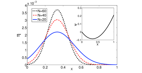
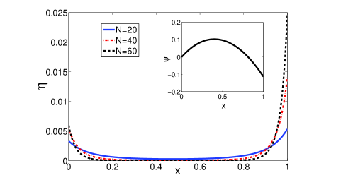
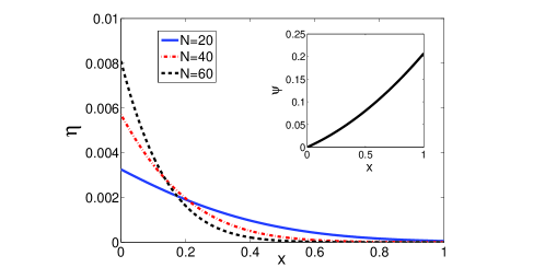
Figure 1:

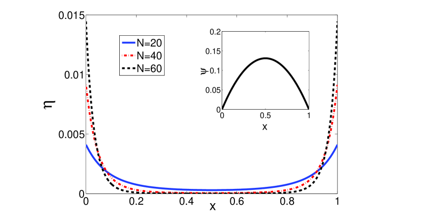
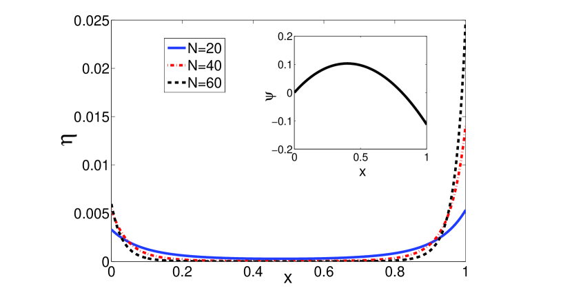
Figure 2:

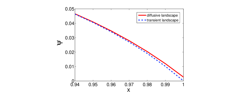
Figure 3:

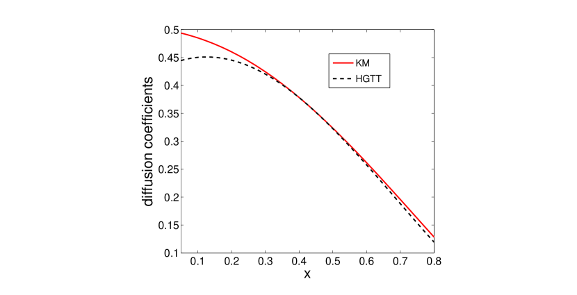
Figure 4:

References

- (1) M. A. Nowak, Evolutionary Dynamics (Harvard University Press, Cambridge, MA, 2006).
- (2) A. Traulsen and C. Hauert, in Reviews of Nonlinear Dynamics and Complexity, edited by H. G. Schuster (Wiley-VCH, Weinheim, 2009).
- (3) C. P. Roca, J. A. Cuesta and A. Sánchez, Phys. Life Rev. 6, 208 (2009).
- (4) R. Durrett, Probability: Theory and Examples (Duxbury Press, Belmont, 1996), second ed.
- (5) S. Karlin and H. M. A. Taylor, A First Course in Stochastic Processes (Academic, London, 1975), second ed.
- (6) R. A. Fisher, Proc. R. Soc. Edinburgh. 42, 321 (1922).
- (7) S. Wright, Genetics. 16, 97 (1931).
- (8) P. A. Moran, The Statistical Processes of Evolutionary Theory (Clarendon, Oxford, 1962).
- (9) M. A. Nowak, A. Sasaki, C. Taylor, and D. Fudenberg, Nature (London) 428, 646 (2004).
- (10) A. Traulsen, J. M. Pacheco and M. A. Nowak, J. Theor. Biol. 246, 522 (2007).
- (11) F. Fu, M. A. Nowak and C. Hauert, J. Theor. Biol. 266, 358 (2010).
- (12) C. Taylor, D. Fudenberg, A. Sasaki and M. A. Nowak, Bull. Math. Biol. 66, 1621 (2004).
- (13) T. Antal and I. Scheuring, Bull. Math. Biol. 68, 1923 (2006).
- (14) C. Taylor, Y. Iwasa, and M. A. Nowak, J. Theor. Biol. 243, 245 (2006).
- (15) H. Ohtsuki, P. Bordalo, and M. A. Nowak, J. Theor. Biol. 249, 289 (2007).
- (16) P. M. Altrock and A. Traulsen, New J. Phys. 11, 013012 (2009).
- (17) B. Wu, P. M. Altrock, L. Wang and A. Traulsen, Phys. Rev. E. 82, 046106 (2010).
- (18) D. Fudenberg, M. A. Nowak, C. Taylor and L. A. Imhof, Theor. Popul. Biol. 70, 352 (2006).
- (19) T. Antal, M. A. Nowak and A. Traulsen, J. Theor. Biol. 257, 340 (2009).
- (20) T. Antal, A. Traulsen, H. Ohtsuki, C. E. Tarnita and M. A. Nowak, J. Theor. Biol. 258, 614 (2009).
- (21) G. Szabó and G. Fáth, Phys. Rep. 446, 97 (2007).
- (22) M. Droz, J. Szwabiński, and G. Szabó, Eur. Phys. J. B 71, 579 (2009).
- (23) G. Szabó, A. Szolnoki, M. Varga, and L. Hanusovszky, Phys. Rev. E 82, 026110 (2010).
- (24) J. Huisman and F. J. Weissing, Nature (London) 402, 407 (1999).
- (25) J. Huisman and F. J. Weissing, Ecology 82, 2682 (2001).
- (26) J. N. Darroch and E. Seneta, J. Appl. Prob. 2, 88 (1965).
- (27) A. Hastings, Trend Ecol. Evol. 19, 39 (2004).
- (28) G. Block and L. J. S. Allen, Bull. Math. Biol. 62, 199 (2000).
- (29) J. C. Claussen and A. Traulsen, Phys. Rev. E 71, 025101(R) (2005).
- (30) Y. Tao and R. Cressman, Bull. Math. Biol. 69, 1377 (2007).
- (31) M. Vellela and H. Qian, Bull. Math. Biol. 69, 1727 (2007).
- (32) S. G. Ficici and J. B. Pollack, J. Theor. Biol. 247, 426 (2007).
- (33) C. M. Grinstead and J. L. Snell, Introduction to probability (American Mathematical Society, Providence, 1997), 2nd edition.
- (34) M. I. Freidlin and A. D. Wentzell, Random Perturbations of Dynamical Systems (Springer, New York, 1984).
- (35) A. Dembo and O. Zeitouni, Large Deviations Techniques and Applications (Springer-Verlag, New York, 1998).
- (36) H. Touchette, Phys. Rep. 478, 1 (2010).
- (37) H. Qian, Nonlinearily. 24, 19 (2011).
- (38) J. Wang, L. Xu and E. K. Wang, Proc. Natl. Acad. Sci. 105, 12271 (2008).
- (39) P. D. Taylor and L. Jonker, Math. Biosci. 40, 145 (1978).
- (40) D. Zhou, B. Wu, H. Ge, J. Theor. Biol. 264, 874 (2010).
- (41) J. Maynard Smith, Evolution and the Theory of Games (Cambridge University Press, Cambridge, 1982).
- (42) H. Ge and H. Qian, Phys. Rev. Lett. 103, 148103 (2009).
- (43) R. G. Strongin and Y. D. Sergeyev, Global Optimization with Non-Convex Constraints: Sequential and Parallel Algorithms (Kluwer Academic Publishers, Dordrecht, 2000).
- (44) W. Feller, Trans. Amer. Math. Soc. 77, 1 (1954).
- (45) C. W. Gardiner, A Handbook of Stochastic Methods: for Physics, Chemistry and the Natural Sciences (Springer, Berlin, 1983).
- (46) W. Y. Tan, Stochastic Modeling of AIDS Epidemiology and HIV Pathogenesis (World Scientific Pub, Singapore, 2000).
- (47) A. Traulsen, J. C. Claussen, and C. Hauert, Phys. Rev. Lett. 95, 238701 (2005).
- (48) F. A. C. C. Chalub and M. O. Souza, Math. Comput. Modell. 47, 743 (2008).
- (49) P. Hänggi, H. Grabert, P. Talkner and H. Thomas, Phys. Rev. A 29, 371 (1984).
- (50) N. G. van Kampen, Stochastic Processes in Physics and Chemistry (Elsevier Science, North-Holland, 1992).
- (51) T. G. Kurtz, Math. Prog. Stud. 5, 67 (1976).
- (52) T. G. Kurtz, Stoch. Proc. Appl. 6, 223 (1978).
- (53) H. Qian, Prot. Sci. 11, 1 (2002).
- (54) I. Nåsell, Math. Biosci. 156, 21 (1999).
- (55) H. Ge and H. Qian, J. Roy. Soc. Interface. 8, 107 (2011).
- (56) J. M. T. Thompson and H. B. Stewart, Nonlinear Dynamics and Chaos (John Wiley, New York, 1986).
- (57) H. K. Khalil, Nonlinear Systems (Prentice Hall, Upper Saddle River NJ, 2002).
- (58) H. Eyring, J. Chem. Phys. 3, 107 (1935).
- (59) H. A. Kramers, Physica. 7, 284 (1949).
- (60) D. Y. Chen, J. F. Feng and M. P. Qian, Science in China (Series A), 39, 7 (1996).
- (61) M. Vellela and H. Qian, J. R. Soc. Interf. 6, 925 (2009).
- (62) H. Qian, P. Z. Shi and J. Xing, Phys. Chem. Chem. Phys. 11, 4861 (2009).
- (63) M. Kimura, Cold Spring Harbour Symp. Quant. Biol. 20, 33 (1955).
- (64) A. J. McKane, D. Waxman, J. Theor. Biol. 247, 849 (2007).
- (65) D. Waxman, J. Theor. Biol. 269, 79 (2011).
- (66) W. H. Sandholm, Population Games and Evolutionary Dynamics (MIT press, Cambridge, MA, 2011).
- (67) P. Ao, Phys. Life Rev. 2, 117 (2005).
- (68) P. Ao, Commun. Theor. Phys. 49, 1073 (2008).
- (69) L. J. S. Allen, An Introduction to Stochastic Processes with Applications to Biology (Prentice Hall, Upper Saddle River, NJ, 2003).
- (70) M. B. Elowitz, A. J. Levine, E. D. Siggia and P. S. Swain, Science 297, 1183 (2002).
- (71) L. Cai, N. Friedman and X. S. Xie, Nature (London) 440, 358 (2006).
- (72) D. A. Beard and H. Qian, Chemical Biophysics: Quantitative Analysis of Cellular Systems (Cambridge University Press, Cambridge, 2008).
- (73) A. Traulsen, J. C. Claussen and C. Hauert, Phys. Rev. E 74, 011901 (2006).
- (74) G. Hu, Zeit. Phys. B, 65, 103 (1986).