Some Exact Results for the Exclusion Process

Abstract

The asymmetric simple exclusion process (ASEP) is a paradigm for non-equilibrium physics that appears as a building block to model various low-dimensional transport phenomena, ranging from intracellular traffic to quantum dots. We review some recent results obtained for the system on a periodic ring by using the Bethe Ansatz. We show that this method allows to derive analytically many properties of the dynamics of the model such as the spectral gap and the generating function of the current. We also discuss the solution of a generalized exclusion process with $N$-species of particles and explain how a geometric construction inspired from queuing theory sheds light on the Matrix Product Representation technique that has been very fruitful to derive exact results for the ASEP.

I Introduction

Equilibrium Statistical Mechanics is a well-established field that embodies Classical Thermodynamics (see e.g. F. Reif, 1965 Reif ). In an extremely terse formulation, this theory could be summarized by saying that the relevant features of the microscopic physics of any system are encoded in a probability measure for which, at thermal equilibrium, a mathematical formula is known. Indeed, a system in contact with a heat bath at temperature $T$ occupies all accessible microscopic configurations ${\mathcal{C}}$ with a probability $P_{{\rm eq}}({\mathcal{C}})$, given by the Boltzmann-Gibbs canonical law:

$${P_{{\rm eq}}({\mathcal{C}})=\frac{{\rm e}^{-E({\mathcal{C}})/kT}}{Z}}\,,$$ (1)

$E({\mathcal{C}})$ being the energy of the configuration ${\mathcal{C}}$. The Partition Function $Z$ (or ‘sum over states’) is related to the thermodynamic Free Energy F via the relation

$${F=-kT{\rm Log}\,Z}\,.$$

This relation is nothing but an avatar of the celebrated Boltzmann law, $S=k\,{\rm Log}\,\Omega$. Macroscopic observables are obtained by taking the expectation values of the corresponding microscopic observables with respect to the canonical measure (1). These postulates provide us with a well-defined prescription to analyze systems at equilibrium. In particular, equilibrium statistical mechanics predicts macroscopic fluctuations (typically Gaussian) that are out of reach of Classical Thermodynamics: the paradigm of such fluctuations is the Brownian Motion.

For systems far from equilibrium, a fundamental theory that would generalize the formalism of equilibrium Statistical Mechanics to time-dependent processes is not yet available. A schematic non-equilibrium process can be represented as a rod in contact with two reservoirs at different temperatures, or at different electrical (chemical) potentials (see Figure 1). In the stationary regime, a constant current flows through the system. Many fundamental questions remain to be answered in order to understand the physics of such a simple system: What are the relevant parameters that would fully characterize the macroscopic state of a non-equilibrium system? Can the stationary state be defined as the optimum of some (unknown) macroscopic functions of some (unknown) parameters? Does a general equation of state exist? Can one classify non-equilibrium processes into ‘Universality classes’? Can one postulate a general form for some non-equilibrium microscopic measures? What do the fluctuations in the vicinity of a stationary state look like?

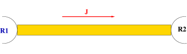
Figure 1: A stationary driven system in contact with two reservoirs at different temperature and/or potential.

A large amount of research has been devoted to these questions and to some related ones. Although the theory is far from being complete, substantial progress has been made, particularly during the last twenty years. There are different ways to try to tackle the profound questions raised above. One line of research consists in exploring structural properties of non-equilibrium systems: this endeavour has led to celebrated results such as Fluctuation Theorems (Gallavotti and Cohen, 1995 Gallavotti ; see also LeboSpohn ), Non-equilibrium Work Relations (Jarzynski, 1997 Jarzynski ) or Macroscopic Fluctuation Theory (G. Jona-Lasinio and co-workers, see e.g. L. Bertini et al. Bertini ).

Another strategy to gain insight into non-equilibrium physics is to extract as much information as possible from analytical studies and from exact solutions of some special models. The Ising model, that has played a fundamental role in the theory of phase transitions, critical exponents and renormalization group, is a landmark of this style of research. In the field of non-equilibrium statistical mechanics, the Asymmetric Simple Exclusion Process (ASEP) is reaching the status of such a paradigm. The ASEP consists of particles on a lattice, that hop from a site to its immediate neighbours, and satisfy the exclusion condition: a given location must be occupied by at most one particle. Therefore, a jump is allowed only if the target site is empty. Physically, the exclusion constraint mimics short-range interactions amongst particles. Besides, in order to drive this lattice gas out of equilibrium, non-vanishing currents must be established in the system. This can be achieved by various means: by starting from non-uniform initial conditions, by coupling the system to external reservoirs that drive currents Krug through the system (transport of particles, energy, heat) or by introducing some intrinsic bias in the dynamics that favors motion in a privileged direction. Then, each particle is an asymmetric random walker that drifts steadily along the direction of an external driving force. Due to its simplicity, this model has appeared in different contexts. It was first proposed as a prototype to describe the dynamics of ribosomes along RNA McDonald1 ; McDonald2 . In the mathematical literature, Brownian processes with hard-core interactions were defined by Spitzer Spitzer who coined the name exclusion process (see also Harris ; Liggett1 ; Liggett2 ). The ASEP also describes transport in low-dimensional systems with strong geometrical constraints MartinRev1 such as macromolecules transiting through capillary vessels TomChou , anisotropic conductors, or quantum dots where electrons hop to vacant locations and repel each other via Coulomb interaction VonOppen . Very popular modern applications of the exclusion process include molecular motors that transport proteins along filaments inside the cells and, of course, ASEP and its variants are ubiquitous in discrete models of traffic flow MartinShock ; Schad . More generally, the ASEP belongs to the class of driven diffusive systems defined by Katz, Lebowitz and Spohn in 1984 KLS . For a general discussion, we refer to e.g., the book of H. Spohn Spohn the review of B. Schmittmann and R. K. P. Zia Zia and that of G. M. Schütz Schutz . An early review of the properties of the ASEP can be found in Derrida, 1998 DerridaRep . We emphasize that the ASEP is defined through dynamical rules: there is no energy associated with a microscopic configuration and thus there is no possibility of writing the stationary measure in the canonical form (1). More generally, the kinetic point of view seems to be a promising and fruitful approach to non-equilibrium systems: for such a presentation of statistical mechanics, we highly recommend to the reader the recent book by P. L. Krapivsky et al. PaulK .

To summarize, the ASEP is a minimal model to study non-equilibrium behaviour (see Figure 2). It is simple enough to allow analytical studies, however it contains the necessary ingredients for the emergence of a non-trivial phenomenology Zia2 :

• ASYMMETRIC: The external driving breaks detailed-balance and creates a stationary current in the system Zia3 . The model exhibits a non-equilibrium stationary state.

• EXCLUSION: The hard core-interaction implies that there is at most 1 particle per site. The ASEP is a genuine N-body problem.

• PROCESS: The dynamics is stochastic and Markovian: there is no underlying Hamiltonian.

Figure 2: The Asymmetric Exclusion Process: A paradigm for non-equilibrium Statistical Mechanics. The particles perform asymmetric random walks $(p\neq q)$ and interact through the exclusion constraint.

The outline of this article is as follows. In section II, we study spectral properties of the ASEP on a ring by using the coordinate Bethe Ansatz. We review the general technique and focus on the TASEP case, which, in our opinion, is one of the simplest models that allows to understand how the Bethe Ansatz method works. In section III, we explain how the fluctuations of the total current in the ASEP can be calculated using a functional formulation of the Bethe Ansatz; we review the exact results obtained and the different scaling regimes that appear in the limit of systems of large sizes. In section IV, we study a generalization of the ASEP in which different classes of particles interact through hierarchical dynamical rules. We show how the steady state of such systems can be determined by using a Matrix Product Representation that involves tensor products of quadratic algebras.

II Spectral Properties of the Markov Matrix

II.1 The model

We consider the exclusion process on a periodic one dimensional lattice with $L$ sites (sites $i$ and $L+i$ are identical) and $N$ particles. Because a lattice site cannot be occupied by more than one particle, the state of a site $i$ ($1\leq i\leq L$) can be characterized by the Boolean number $\tau_{i}=0,1$ according as the site $i$ is empty or occupied.

The system evolves in continuous time according to the following stochastic rule: a particle on a site $i$ at time $t$ jumps, in the interval between $t$ and $t+dt$, with probability $dt$ to the neighbouring site $i+1$ if this site is empty (exclusion rule) and with probability $x\ dt$ to the site $i-1$ if this site is empty (see Figure 3). In the totally asymmetric exclusion process (TASEP) the jumps are totally biased in one direction ($x=0$). On the other hand, the symmetric exclusion process (SEP) corresponds to the choice $x=1$.

The number $N$ of particles is conserved by the dynamics. The total number of configurations for $N$ particles on a ring with $L$ sites is given by $\Omega=L!/[N!(L-N)!]$.

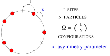
Figure 3: The Asymmetric Exclusion Process on a Ring.

A configuration $\mathcal{C}$ can be represented by the sequence $(\tau_{1},\tau_{2},\ldots,\tau_{L}).$ We call $P_{t}(\mathcal{C})$ the probability of configuration $\mathcal{C}$ at time $t$. As the exclusion process is a continuous-time Markov process, the time evolution of $P_{t}(\mathcal{C})$ is determined by the master equation

$$\frac{d}{dt}P_{t}(\mathcal{C})=\sum_{\mathcal{C}^{\prime}}M(\mathcal{C},\mathcal{C}^{\prime})P_{t}(\mathcal{C}^{\prime})\,.$$ (2)

The Markov matrix $M$ encodes the dynamics of the exclusion process: the element $M(\mathcal{C},\mathcal{C}^{\prime})$ is the transition rate from configuration $\mathcal{C}^{\prime}$ to $\mathcal{C}$ and the diagonal term $M(\mathcal{C},\mathcal{C})=-\sum_{\mathcal{C}^{\prime}}M(\mathcal{C}^{\prime},\mathcal{C})$ represents the exit rate from configuration $\mathcal{C}$.

A right eigenvector $\psi$ is associated with the eigenvalue $E$ of $M$ if

$$M\psi=E\psi\,.$$ (3)

The matrix $M$ is a real non-symmetric matrix and, therefore, its eigenvalues (and eigenvectors) are either real numbers or complex conjugate pairs. The spectrum of $M$ contains the eigenvalue $E=0$ and the associated right eigenvector is the stationary state. For the ASEP on a ring the steady state is uniform and all configurations have the same probability $1/\Omega$ DerridaRep .

Because the dynamics is ergodic (i.e., $M$ is irreducible and aperiodic), the Perron-Frobenius theorem (see, for example, Gantmacher 1959 Gantmacher ) implies that 0 is a non-degenerate eigenvalue and that all other eigenvalues $E$ have a strictly negative real part; the relaxation time of the corresponding eigenmode is $\tau=-1/\mathrm{Re}(E)$. The imaginary part of $E$ gives rise to an oscillatory behaviour.

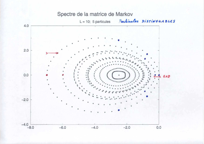
Figure 4: Example of a spectrum of a Markov matrix for the TASEP with $N=5$ distinguishable particles and a ring of $L=10$ sites. The thick dots indicate some of the eigenvalues that correspond to the indistinguishable case.

In Figure 4, we display the example of a spectrum of a Markov matrix for the TASEP with $N=5$ distinguishable particles and a ring of $L=10$ sites. In this case, the dimension of the phase space is 1260. However, when the particles are indistinguishable, the dimension of the Markov matrix is reduced by a factor of $N=5$ and is given by 252. The spectrum of the indistinguishable case is included in the larger spectrum of the distinguishable problem.

II.2 The Bethe Ansatz

Another way to characterize a configuration is to specify the positions of the $N$ particles on the ring, $(\xi_{1},\xi_{2},\dots,\xi_{N})$ with $1\leq\xi_{1}<\xi_{2}<\dots<\xi_{N}\leq L$. In this representation, the eigenvalue equation (3) becomes

$$E\psi(\xi_{1},\dots,\xi_{N})=$$

$$\sum_{i}\left[\psi(\xi_{1},\dots,\xi_{i-1},\ \xi_{i}-1,\ \xi_{i+1},\dots,\xi_{N})-\psi(\xi_{1},\dots,\xi_{N})\right]$$

$$+ \sum_{j}x\left[\psi(\xi_{1},\dots,\xi_{j-1},\ \xi_{j}+1,\ \xi_{j+1},\dots,\xi_{N})-\psi(\xi_{1},\dots,\xi_{N})\right]\,,$$ (4)

where the sums run over the indexes $i$ such that $\xi_{i-1}<\xi_{i}-1$ and over the indexes $j$ such that $\xi_{j}+1<\xi_{j+1}$. In other words, the sums are restricted to jumps that respect the exclusion condition DerridaRep .

Since the works of Dhar 1987 Dhar , and Gwa and Spohn 1992 Gwa , it is known that the Bethe Ansatz can be applied to the ASEP. The idea of the Bethe Ansatz (H. Bethe 1931 Bethe ) consists in writing the eigenvectors $\psi$ of the Markov matrix as linear combinations of plane waves:

$$\psi(\xi_{1},\dots,\xi_{N})=\sum_{\sigma\in\Sigma_{N}}A_{\sigma}\,z_{\sigma(1)}^{\xi_{1}}\,z_{\sigma(2)}^{\xi_{2}}\dots z_{\sigma(N)}^{\xi_{N}}\,,$$ (5)

where $\Sigma_{N}$ is the group of the $N!$ permutations of $N$ indexes. The coefficients $\{A_{\sigma}\}$ and the wave-numbers $\{z_{1},\dots,z_{N}\}$ are complex numbers to be determined. We observe that in the case where all particles are far from each other (i.e. no particles are located on adjacent sites so that $\xi_{k-1}<\xi_{k}-1$ for all $k=1,\ldots N$), each monomial that appears on the right hand side of the expression of the Bethe wave function is a solution of the eigen-equation (4), with an eigenvalue $E$ given by

$$E(z_{1},z_{2}\ldots z_{N})=\sum_{i=1}^{N}\frac{1}{z_{i}}+x\sum_{i=1}^{N}z_{i}\,-N(1+x)\,.$$ (6)

However, in order for the trial wave function to be a genuine eigenfunction, equation (4) must be fulfilled for all configurations: therefore, one has to insure that when two or more particles are adjacent equation (4) is still satisfied. The case where exactly two particles are adjacent and all other particles are well separated from one another is enough to fix the value of all the $A_{\sigma}$’s (up to an overall multiplicative constant). In other words, the form of the Bethe wave-function (5) is fully determined by the ‘two-body collisions’. However, more particles can form larger clusters: this corresponds to $k$-body collisions with $2<k\leq N$: such collisions impose further constraints that the Bethe wave-function has no reasons, a priori, to satisfy. Fortunately, in the present problem, the constraints imposed by the $k$-body collisions can be written as linear combinations of the two-body constraints and are therefore automatically satisfied by the Bethe wave-function. In the Bethe Ansatz jargon, this fact is formulated by saying that the $3$-body collisions factorize into $2$-body collisions etc… This remarkable property, that can be verified explicitly in the case of equation (4), lies at the heart of the integrability of the exclusion process, i.e., it implies that the ASEP can be solved by Bethe Ansatz. In fact, the ASEP can be mapped exactly into well-studied systems such as quantum spin chains Alcaraz ; Albertini , vertex models Baxter ; Kandel ; VanBeij2 or solid-on-solid models Rajesh which are well-known to be integrable.

Because we are studying the system on a homogeneous ring, the function $\psi$ must also satisfy the following periodic boundary conditions

$$\psi(\xi_{1},\xi_{2},\dots,\xi_{n})=\psi(\xi_{2},\dots,\xi_{n},\xi_{1}+L)\,.$$ (7)

These periodic conditions quantify the eigenvalues by imposing a set of equations satisfied by the $z_{i}$’s, the Bethe Equations:

$$z_{i}^{L}=(-1)^{N-1}\prod_{j=1}^{N}\frac{xz_{i}z_{j}-(1+x)z_{i}+1}{xz_{i}z_{j}-(1+x)z_{j}+1}\,.$$ (8)

This set of non-linear algebraic equations must be satisfied by the fugacities. Therefore, in order to obtain the spectrum of the ASEP Markov matrix one has first to find all $N$-tuplets $(z_{1},z_{2},\ldots,z_{N})$ that solve the Bethe equations (8). Then, given a solution, one can calculate the corresponding eigenvalue (6) and eigenfunction (5). Of course, in practice this program can be carried out only in some special situations (for example in a limited portion of the spectrum) and usually one has to take the ‘thermodynamic’ limit $L,N\to\infty$ with a fixed value of the density $\rho=N/L$. Besides, the completeness issue (i.e. whether the Bethe Ansatz does provide the full spectrum) is a difficult problem in algebraic geometry Baxtervertex ; Langlands .

II.3 Bethe Equations for the TASEP

The totally asymmetric exclusion process (TASEP), that corresponds to $x=0$, provides a particularly instructive illustration of the Bethe Ansatz. The Bethe equations take a simpler form on which analytical calculations can be carried out even for finite values of $L$ and $N$. The TASEP is one of the simplest non-trivial models that allows to understand how the Bethe Ansatz technique works. In this subsection, we present a complete and self-contained derivation of the Bethe Ansatz for the TASEP.

First, we show that the Bethe wave function $\psi$ of the TASEP can be written as a determinant ogkm2 . The form of this determinant can be guessed heuristically by working out explicitly examples for small systems. Here, we reverse the logic and define $\psi$ as

$$\psi(\xi_{1},\dots,\xi_{N})=\det(R)\,,$$ (9)

where $R$ is a $N\times N$ matrix with elements

$$R(i,j)=\frac{z_{i}^{\xi_{j}}}{(1-z_{i})^{j}}\ \ \mbox{for }1\leq i,j\leq N\,,$$ (10)

$(z_{1},\dots,z_{N})$ being $N$ complex numbers. By expanding the determinant, one recovers the generic form (5) for the Bethe wave function $\psi$. We now show that $\psi$, thus defined, is a solution of the eigenvalue equation (4) with $x=0$. First, we need to prove that $\psi$ satisfies two identities which are valid for any values of $z_{i}$ and of $\xi_{i}$. The first identity is

$$E\psi(\xi_{1},\dots,\xi_{N})=\sum_{k=1}^{N}[\psi(\xi_{1},\dots,\xi_{k}-1,\dots,\xi_{N})-\psi(\xi_{1},\dots,\xi_{k},\dots,\xi_{N})]\,,$$ (11)

where $E$ is given by $E=-N+\sum_{i=1}^{N}1/z_{i}\,.$ We emphasize that this equality is true for any $(\xi_{1},\dots,\xi_{N})$ and $(z_{1},\dots,z_{N})$ without imposing the ordering $1\leq\xi_{1}<\xi_{2}<\dots<\xi_{N}\leq L$. Besides, $k$ runs from 1 to $N$ without any restriction, i.e. we do not impose that $\xi_{k-1}<\xi_{k}-1$. Equation (11) is proved by writing

$$\psi(\xi_{1},\dots,\xi_{k}-1,\dots,\xi_{N})-\psi(\xi_{1},\dots,\xi_{k},\dots,\xi_{N})=$$

$$\det\left(R(i,1),\dots,\left(\frac{1}{z_{i}}-1\right)R(i,k),\dots,R(i,N)\ \right)\,.$$ (12)

This determinant is similar to $\det(R)$ except for the $k$-th column. Expanding this determinant over all permutations of $\{1,\dots,N\}$ and performing the sum over $k=1,\dots,N$ leads to the desired equation. The second identity takes care of the two particles collision case: it is valid for any $(z_{1},\dots,z_{N})$ and any $(\xi_{1},\dots,\xi_{N})$ with $\xi_{k-1}=\xi_{k}$, and is given by

$$\psi(\xi_{1},\dots,\xi_{k},\xi_{k},\dots,\xi_{n})-\psi(\xi_{1},\dots,\xi_{k},\xi_{k}+1,\dots,\xi_{n})=0\,.$$ (13)

This identity is proved as follows: we rewrite the left hand side of equation (13) as the determinant $\det(\tilde{R})$ where $\tilde{R}$ is a matrix that is identical to $R$ except for its $k$-th column that is given by

$$\tilde{R}(i,k)=\frac{z_{i}^{\xi_{k}}-z_{i}^{\xi_{k}+1}}{(1-z_{i})^{k}}=\frac{z_{i}^{\xi_{k}}}{(1-z_{i})^{k-1}}=R(i,k-1)=\tilde{R}(i,k-1)\,.$$ (14)

We remark that the $(k-1)$-th and the $k$-th columns of $\tilde{R}$ are equal and, therefore, $\det(\tilde{R})=0$, proving equation (13).

To conclude, we note that the eigenvalue equation (4) is similar to equation (11) except that in (4) the sum is restricted to the allowed jumps of particles, i.e., to the values of $k$ such that $\xi_{k-1}+1<\xi_{k}$. However, in equation (11), the terms with $\xi_{k-1}+1=\xi_{k}$ vanish thanks to equation (13). Hence, equation (11) is in fact exactly the same as the eigenvalue equation when the eigenvector has the form assumed in equations (9, 10).

Finally, because of the periodic boundary conditions (7), the $z_{i}$’s are quantified by the Bethe equations, that we now rederive. Denoting by $i$ and $j$ the generic line and column of the matrix $R$, we can write

$$\psi(\xi_{2},\dots,\xi_{N},\xi_{1}+L)=\det\left(\frac{z_{i}^{\xi_{2}}}{1-z_{i}},\dots,\frac{z_{i}^{\xi_{j+1}}}{(1-z_{i})^{j}},\dots,\frac{z_{i}^{\xi_{1}+L}}{(1-z_{i})^{N}}\right)\,.$$ (15)

By cyclic permutation of the columns, we obtain

$$\psi(\xi_{2},\dots,\xi_{N},\xi_{1}+L)$$ (16)

$$= (-1)^{N-1}\det\left(\frac{z_{i}^{\xi_{1}+L}}{(1-z_{i})^{N}},\frac{z_{i}^{\xi_{2}}}{1-z_{i}},\dots,\frac{z_{i}^{\xi_{j}}}{(1-z_{i})^{j-1}},\dots\right)$$

$$= (-1)^{N-1}\det\left(\frac{z_{i}^{L}}{(1-z_{i})^{N-1}}\,R(i,1),\dots,(1-z_{i})\,R(i,j),\dots\right)$$

$$= (-1)^{N-1}\prod_{k=1}^{N}(1-z_{k})\,\,\,\ \det\left(\frac{z_{i}^{L}}{(1-z_{i})^{N}}\,R(i,1),\dots,R(i,j),\dots\right)\,.$$

The last expression will be equal to $\psi(\xi_{1},\xi_{2},\dots,\xi_{n})=\det(R)\,$ if $z_{1},\dots,z_{N}$ are solutions of the TASEP Bethe equations:

$$(z_{i}-1)^{N}z_{i}^{-L}=-\prod_{k=1}^{N}(1-z_{k})\ \ \ \hbox{for}\ \ \ i=1,\dots,N\,.$$ (17)

These equations can of course be obtained by substituting $x=0$ in the general Bethe equations (8) for ASEP. We note that determinantal representations of the eigenvectors and of the exact probability distribution at finite time play an important role in the study of the TASEP since the seminal work of G. M. Schütz SchutzBA , that has been generalized further by V. B. Priezzhev Priezzhev and N. M. Bogoliubov Bogoliubov (see e.g. the review of V. B. Priezzhev 2005 PriezzhevInde ).

II.4 Analysis of the TASEP Bethe Equations

The Bethe equations for the TASEP exhibit a remarkable ‘decoupling’ property that allows to perform analytical calculations even for finite values of $L$ and $N$. Using the auxiliary variables $Z_{i}=2/z_{i}-1$, the Bethe equations (17) become

$$(1-Z_{i})^{N}\ (1+Z_{i})^{L-N}=-2^{L}\prod_{j=1}^{N}\frac{Z_{j}-1}{Z_{j}+1}\ \ \ \hbox{for}\ \ \ i=1,\dots,N\,.$$ (18)

We note that the right-hand side of these equations is independent of the index $i$: this property is true only for the TASEP where the Bethe equations decouple and can be reduced to a polynomial in one-variable plus a self-consistency equation as shall be explained below. The corresponding eigenvalue $E$ of the Markov matrix $M$ is given by

$$2E=-N+\sum_{j=1}^{N}Z_{j}\,.$$ (19)

The solutions of the Bethe equations (18) are the roots of the polynomial equation of degree $L$

$$(1-Z)^{N}(1+Z)^{L-N}=Y\,,$$ (20)

where $Y$ is determined self-consistently by the r.h.s. of equation (18). Given an arbitrary value of the complex number $Y$, the roots of the polynomial (20) display a simple geometrical layout. If we write $Y=r^{L}\,e^{i\phi}$, $r$ being a positive real number, we observe that equation (20) implies that

$$|Z-1|^{\rho}|Z+1|^{1-\rho}=r$$ (21)

where $\rho=N/L$ is the particle density in the system. The curves defined in the complex plane for $0<r<\infty$ are known as Cassini ovals (see Figure 5). As can be seen in Fig. 5, the topology of the Cassini ovals depends on the value of $r$ with a critical value:

$$r_{c}=2\rho^{\rho}(1-\rho)^{1-\rho}\,.$$ (22)

For $r<r_{c}$, the curve consists of two disjoint ovals with $N$ solutions on the oval surrounding $+1$ and $L-N$ solutions on the oval surrounding $-1$. For $r=r_{c}$, the curve is a deformed Bernoulli lemniscate with a double point at $Z_{c}=1-2\rho$. For $r>r_{c}$, the curve is a single loop with $L$ solutions. Note that the Cassini ovals are symmetrical only if $\rho=1/2$; in this case $r_{c}=1.$

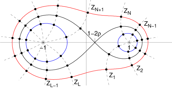
Figure 5: The loci of the roots of the Bethe Equations for the TASEP are given by Cassini Ovals.

This geometric layout leads to the following procedure for solving the Bethe Equations for the TASEP (for a review see e.g. ogkmrev ):

• SOLVE, for any given value of $Y$, the equation $\,\,\,(1-z_{i})^{N}(1+z_{i})^{L-N}=Y\,.$ The roots are located on Cassini Ovals

• CHOOSE $N$ roots $z_{c(1)},\ldots z_{c(N)}$ amongst the $L$ available roots, with a choice set $c:\{c(1),\ldots,c(N)\}\subset\{1,\ldots,L\}\,.$

• SOLVE the self-consistent equation ${\bf A_{c}(Y)=Y}$ where

  $$A_{c}(Y)=-2^{L}\prod_{j=1}^{N}\frac{z_{c(j)}-1}{z_{c(j)}+1}\,.$$

• DEDUCE from the value of $Y$, the $z_{c(j)}$’s and the energy corresponding to the choice set $c$ :

  $$2E_{c}(Y)=-N+\sum_{j=1}^{N}z_{c(j)}.$$

Eigenvalues of the Markov matrix are thus related to the choice sets of roots on the Cassini ovals; there is a strong evidence ogkmrev that choice sets are in one-to-one correspondence with the eigenvalues of the Markov matrix. A simple argument is that the total number of choice sets is given by $\Omega=L!/[N!(L-N)!]$ which is precisely the size of the Markov matrix.

The choice function $c_{0}(j)=j$ that selects the $N$ fugacities $Z_{i}$ with the largest real parts (see Figure 5) provides the ground state of the Markov matrix. The spectral gap, given by the first excited eigenvalue, corresponds to the choice $c_{1}(j)=j$ for $j=1,\ldots,N-1$ and $c_{1}(N)=N+1$ Gwa . For this choice set, the calculation can be carried out explicitly and one can show that, in the large $L$ limit, the first excited state is given by a solution of a transcendental equation. For a density $\rho$, one obtains

$$E_{1}= {-2\sqrt{\rho(1-\rho)}\frac{6.509189337\ldots}{L^{3/2}}}\pm{\frac{2i\pi(2\rho-1)}{L}\,.}$$

$$\,\,\,\,\,\,\,\,\,\,\,\,\,\,\,\,{\rm{(RELAXATION)}}\,\,\,\,\,\,\,\,\,\,\,\,\,\,\,\,\,\,\,\,{\rm{(OSCILLATIONS)}}$$

The first excited state consists of a pair of conjugate complex numbers when $\rho$ is different from 1/2. The real part of $E_{1}$ describes the relaxation towards the stationary state: we find that the largest relaxation time scales as $T\sim L^{z}$ with the dynamical exponent $z=3/2$ VanBSpohn ; Dhar ; Gwa ; Kim1 ; ogkm1 . This value agrees with the dynamical exponent of the one-dimensional Kardar-Parisi-Zhang equation that belongs to the same universality class as ASEP (see the review of Halpin-Healy and Zhang 1995 HHZ ). The imaginary part of $E_{1}$ represents the relaxation oscillations and scales as $L^{-1}$; these oscillations correspond to a kinematic wave that propagates with the group velocity $2\rho-1$: such traveling waves can be probed by dynamical correlations Majumdar ; Barma .

The same procedure also allows to classify the higher excitations in the spectrum deGier2 . For the partially asymmetric case ($x\neq 0$), the Bethe equations do not decouple and analytical results are much harder to obtain. A systematic procedure for calculating the finite size corrections of the upper region of the ASEP spectrum was developed by Doochul Kim Kim1 ; Kim2 .

We emphasize that the results presented here are valid for the ASEP on a finite periodic lattice. Problems with open boundary conditions deGier1 ; deGier2 ; deGier3 or on infinite lattices Sasamoto require different approaches. In particular, the exclusion process on the infinite line has fascinating connections with random matrix theory and with the Robinson-Schensted-Knuth correspondence. More precisely, consider the totally asymmetric case and suppose that the initial configuration of the TASEP is such that all sites $i\leq 0$ are occupied and all sites with $i>0$ are empty. Then, the probability that a particle initially at $-m$ moves at least $n$ steps to the right in time $t$ equals the probability distribution of the largest eigenvalue in a unitary Laguerre random matrix ensemble. This crucial fact, first understood by Johannson in 2000 Johansson , allows to relate the statistical properties of the totally asymmetric exclusion process to the classical Tracy-Widom laws TracyWidom for the largest eigenvalue in ensembles of random matrices. The study of such relations has become a subfield per se and has stimulated many works (see e.g., SpohnInde ; SpohnCours ; FerrariPatrick ). In particular, the determinantal representation of the transition probabilities of the TASEP allows to retrieve Johannson’s result in a very appealing manner Rakos . More recently, in a series of articles Tracy1 ; Tracy2 ; Tracy3 ; Tracy4 ; Tracy5 , C. A. Tracy and H. Widom have found some integral formulas for the probability distribution of an individual particle starting from step initial conditions in the asymmetric exclusion process with general parameter values (i.e. allowing forward and backward jumps). These expressions can be rewritten as a single integral involving a Fredholm determinant, that is amenable to asymptotic analysis. In particular, a limit theorem is proven for the total current distribution. These breakthroughs extend the results of Johansson on TASEP to ASEP: this is a crucial progress because the weakly asymmetric process leads to a well-defined continuous limit. In particular, a very important outgrow of these studies are the recent papers of H. Spohn, T. Sasamoto and S. Prolhac, in which the height fluctuations of the Kardar-Parisi-Zhang equation and $n$-point correlation functions are exactly derived, solving a problem that remained open for 25 years (see the articles of H. Spohn and T. Sasamoto, and of P. L. Ferrari in the present special issue). For an overview of all these fascinating problems, we refer the reader to the recent review article by Kriecherbauer and Krug 2010 Kriecherbauer .

Finally, we note that the Bethe Ansatz can be used in models that are closely related to the ASEP, such as the zero-range process Povolotsky , the raise and peel model AlcarazRitt , vicious walkers Dorlas or the Bernoulli matching model of sequence alignment PriezSchutz .

III Fluctuations of the total current

In this section, we explain how the statistics of the total current FerrariFontes ; VanBeij3 in the ASEP on a ring can be determined by the Bethe Ansatz. In particular, we show that the fluctuations of the current can display a non-Gaussian behaviour in contrast with the equilibrium case.

III.1 Current statistics and Bethe Ansatz

We call $Y_{t}$ the total distance covered by all the particles between time 0 and time $t$ and define $P_{t}(\mathcal{C},Y)$ the joint probability of being in the configuration $\mathcal{C}$ at time $t$ and having $Y_{t}=Y$. The evolution equation of $P_{t}(\mathcal{C},Y)$ is:

$$\frac{d}{dt}P_{t}(\mathcal{C},Y)=\sum_{\mathcal{C}^{\prime}}\Big{(}M_{0}(\mathcal{C},\mathcal{C}^{\prime})P_{t}(\mathcal{C}^{\prime},Y)+M_{1}(\mathcal{C},\mathcal{C}^{\prime})P_{t}(\mathcal{C}^{\prime},Y-1)+M_{-1}(\mathcal{C},\mathcal{C}^{\prime})P_{t}(\mathcal{C}^{\prime},Y+1)\Big{)}\,.$$ (23)

Using the generating function $F_{t}(\mathcal{C})$

$$F_{t}(\mathcal{C})=\sum_{Y=0}^{\infty}{\rm e}^{\gamma Y}P_{t}(\mathcal{C},Y)\,,$$ (24)

the evolution equation becomes

$$\frac{d}{dt}F_{t}(\mathcal{C})=\sum_{\mathcal{C}^{\prime}}\Big{(}M_{0}(\mathcal{C},\mathcal{C}^{\prime})+{\rm e}^{\gamma}M_{1}(\mathcal{C},\mathcal{C}^{\prime})+{\rm e}^{-\gamma}M_{-1}(\mathcal{C},\mathcal{C}^{\prime})\Big{)}F_{t}(\mathcal{C}^{\prime})=\sum_{\mathcal{C}^{\prime}}M(\gamma)(\mathcal{C},\mathcal{C}^{\prime})F_{t}(\mathcal{C}^{\prime})\,.$$ (25)

This equation is similar to the original Markov equation (2) for the probability distribution $\psi_{t}(\mathcal{C})$ but now the original Markov matrix $M$ is deformed by a jump-counting fugacity ${\gamma}$ into $M(\gamma)$ (which is not a Markov matrix in general), given by

$$M(\gamma)=M_{0}+{\rm e}^{\gamma}M_{1}+{\rm e}^{-\gamma}M_{-1}\,.$$ (26)

In the long time limit, $t\to\infty$, the behaviour of $F_{t}(\mathcal{C})$ is dominated by the largest eigenvalue $E(\gamma)$ and one can write

$${\left\langle{\rm e}^{\gamma Y_{t}}\right\rangle\simeq{\rm e}^{E(\gamma)t}}\,.$$ (27)

Thus, in the long time limit, the function $E(\gamma)$ is the generating function of the cumulants of the total current $Y_{t}$. But $E(\gamma)$ is also the dominant eigenvalue of the matrix $M(\gamma)$. Therefore, the current statistics has been traded into an eigenvalue problem. Fortunately, the deformed matrix $M(\gamma)$ can still be diagonalized by the Bethe Ansatz. In fact, a small modification of the calculations described in Section II leads to the following Bethe Ansatz equations

$$z_{i}^{L}=(-1)^{N-1}\prod_{j=1}^{N}\frac{x{\rm e}^{-\gamma}z_{i}z_{j}-(1+x)z_{i}+{\rm e}^{\gamma}}{x{\rm e}^{-\gamma}z_{i}z_{j}-(1+x)z_{j}+{\rm e}^{\gamma}}\,.$$ (28)

The eigenvalues of $M(\gamma)$ are given by

$$E(\gamma;z_{1},z_{2}\ldots z_{N})={\rm e}^{\gamma}\sum_{i=1}^{N}\frac{1}{z_{i}}+x{\rm e}^{-\gamma}\sum_{i=1}^{N}z_{i}\,-N(1+x)\,.$$ (29)

The cumulant generating function corresponds to the largest eigenvalue.

Remark: One can define ${G(j)}$, the large-deviation function of the current, as follows

$$Prob\left(\frac{Y_{t}}{t}=j\right){\sim}e^{-tG(j)}\,.$$ (30)

It can be shown using (27) that $G(j)$ and $E(\gamma)$ are the Legendre transforms of each other. Large deviation functions play an increasingly important role in non-equilibrium statistical physics (see H. Touchette 2009 Touchette ), in particular in relation to the Fluctuation Theorem LeboSpohn . Thus, determining exact expression for these large deviation functions for interacting particle processes, either analytically or numerically is a major challenge in the field (we refer the reader to the review of B. Derrida, 2007 DerrReview ). Besides, higher cumulants of the current and large deviations are also of experimental interest in relation to counting statistics in quantum systems Flindt .

III.2 The TASEP Case

For the TASEP, the Bethe equations (28) decouple and can be studied by using the procedure outlined in Section II.4. The $x=0$ case was completely solved by B. Derrida and J. L. Lebowitz in 1998 DLeb . These authors calculated $E(\gamma)$ by Bethe Ansatz to all orders in $\gamma$. More precisely, they obtained the following representation of the function $E(\gamma)$ in terms of an auxiliary parameter $B$:

$$E(\gamma) = -N\sum_{k=1}^{\infty}\left(\begin{array}[]{c}kL-1\\ kN\end{array}\right)\frac{B^{k}}{kL-1}\,,$$ (33)

$$\gamma = -\sum_{k=1}^{\infty}\left(\begin{array}[]{c}kL\\ kN\end{array}\right)\frac{B^{k}}{kL}\,.$$ (36)

These expressions allow to calculate the cumulants of $Y_{t}$, for example the mean-current $J$ and the diffusion constant $D$:

$$J=\lim_{t\to\infty}\frac{\langle Y_{t}\rangle}{t} = \frac{{\rm d}E(\gamma)}{{\rm d}\gamma}\Big{|}_{\gamma=0}=\frac{N(L-N)}{L-1}\,,$$ (37)

$$\,\,\,D=\lim_{t\to\infty}\frac{\langle Y_{t}^{2}\rangle-\langle Y_{t}\rangle^{2}}{t} = \frac{{\rm d}^{2}E(\gamma)}{{\rm d}\gamma^{2}}\Big{|}_{\gamma=0}=\frac{N^{2}\;(2L-3)!\;(N-1)!^{2}\;(L-N)!^{2}}{(L-1)!^{2}\;(2N-1)!\;(2L-2N-1)!}\,.$$ (38)

When $L\to\infty$, with a fixed density $\rho=L/N$ and $|j-L\rho(1-\rho)|\ll L$, the large deviation function $G(j)$, defined in (30) can be written in the following scaling form:

$$G(j)=\sqrt{\frac{\rho(1-\rho)}{\pi N^{3}}}H\Big{(}\frac{j-L\rho(1-\rho)}{\rho(1-\rho)}\Big{)}$$ (39)

with

$$H(y)\simeq-\frac{2\sqrt{3}}{5\sqrt{\pi}}y^{5/2}\,\,\,\, \,\,\,\,y\to+\infty\,,$$ for (40)

$$H(y)\simeq-\frac{4\sqrt{\pi}}{3}|y|^{3/2}\,\,\,\, \,\,\,\,y\to-\infty\,.$$ for (41)

This large deviation function is not a quadratic polynomial, even in the vicinity of the steady state. Moreover, the shape of this function is skew: it decays as the exponential of a power law with an exponent $5/2$ for $y\to+\infty$ and with an exponent $3/2$ for $y\to-\infty$.

III.3 The general case: Functional Bethe Ansatz

In the general case $x\neq 0$, the Bethe Ansatz equations do not decouple and a procedure for solving them was lacking. For example, it did not even seem possible to extract from the Bethe equations (28) a formula for the mean stationary current (which can be obtained very easily by other means from the fact that the stationary measure is uniform). Finally, the solution was found by rewriting the Bethe Ansatz as a functional equation and restating it as a purely algebraic problem. We explain here the method we followed Sylvain1 ; Sylvain3 and describe some of the results obtained. First, we perform the following change of variables,

$$y_{i}=\frac{1-{\rm e}^{-\gamma}z_{i}}{1-x{\rm e}^{-\gamma}z_{i}}\,.$$ (42)

In terms of the variables $y_{i}$ the Bethe equations read

$${\rm e}^{L\gamma}\left(\frac{1-y_{i}}{1-xy_{i}}\right)^{L}=-\prod_{j=1}^{N}\frac{y_{i}-xy_{j}}{xy_{i}-y_{j}}\,\,\,\,{\rm for}\,\,\,\,i=1\ldots N\,.$$ (43)

Here again the equations do not decouple as soon as $x\neq 0$. However, these equations are now built from first order monomials in the $y_{i}$’s and they are symmetrical in these variables. This observation suggests to introduce an auxiliary variable ${\bf T}$ that plays the same role with respect to all the $y_{i}$’s and allows to define the auxiliary equation:

$${\rm e}^{L\gamma}\left(\frac{1-{\bf T}}{1-x{\bf T}}\right)^{L}=-\prod_{j=1}^{N}\frac{{\bf T}-xy_{j}}{x{\bf T}-y_{j}}\,\,\,\,{\rm for}\,\,\,\,i=1\ldots N\,.$$ (44)

This equation, in which ${\bf T}$ is the unknown, and the $y_{i}$’s are parameters, can be rewritten as a polynomial equation:

$$P(T)={\rm e}^{L\gamma}(1-T)^{L}{\prod_{i=1}^{N}(xT-y_{i})}+(1-xT)^{L}{\prod_{i=1}^{N}(T-xy_{i})}=0\,.$$ (45)

Because the Bethe equations (43) imply that $P(y_{i})=0$ for $i=1\ldots N\,$, the polynomial $Q(T)$, defined as

$$Q(T)=\prod\limits_{i=1}^{N}(T-y_{i})\,,$$ (46)

must divide the polynomial $P(T)$. Now, if we examine closely the expression of $P(T)$, we observe that the factors that contain the $y_{i}$’s inside the products over $i$ can be written in terms of $Q(T)$. Therefore, we conclude that $Q(T)$ DIVIDES $e^{L\gamma}(1-T)^{L}Q(xT)+(1-xT)^{L}x^{N}Q(T/x).$ Equivalently, there exists a polynomial ${R(T)}$ such that

$$Q(T)R(T)=e^{L\gamma}(1-T)^{L}Q(xT)+x^{N}(1-xT)^{L}Q(T/x)\,.$$ (47)

This functional equation is equivalent to the Bethe Ansatz equations (it is also known as Baxter’s TQ equation). It can be used to determine the polynomial ${Q(T)}$ of degree ${N}$ that vanishes at the Bethe roots. In the present case, equation (47) can be solved perturbatively w.r.t. ${\gamma}$ to any desired order. Knowing ${Q(T)}$ perturbatively an expansion of ${E(\gamma)}$ is derived, leading to the cumulants of the current and to the large deviation function. For example, this method allows to calculate the following cumulants of the total current:

${\bullet}$ Mean Current $J$: $J=(1-x)\frac{N(L-N)}{L-1}\sim(1-x)L\rho(1-\rho)\,\hbox{ for }\,\,L\rightarrow\infty\,.$

${\bullet}$ Diffusion Constant $D$:

$${D=(1-x)\frac{2L}{L-1}\sum_{k>0}{k^{2}\frac{C_{L}^{N+k}}{C_{L}^{N}}\frac{C_{L}^{N-k}}{C_{L}^{N}}\left(\frac{1+x^{k}}{1-x^{k}}\right)}}\,.$$

(We note that this formula was previously derived DMal using the Matrix Product Representation that we discuss in the next section). In the limit of a large system size, ${L\rightarrow\infty}$, with asymmetry parameter ${x\rightarrow 1}$ and with a fixed value of ${\phi=\frac{(1-x)\sqrt{L\rho(1-\rho)}}{2}}$, the diffusion constant assumes a simple expression

$${D\sim 4\phi L\rho(1-\rho)\int_{0}^{\infty}du\frac{u^{2}}{\tanh{\phi u}}e^{-u^{2}}}.$$

${\bullet}$ Third cumulant: the Skewness measures the non-Gaussian character of the fluctuations. An exact combinatorial expression of the third moment, valid for any values of $L$, $N$ and $x$, was calculated by S. Prolhac in Sylvain2 . It is given by

$$\frac{E_{3}}{6L^{2}} = \frac{1-x}{L-1}\sum_{i>0}\sum_{j>0}\frac{C_{L}^{N+i}C_{L}^{N-i}C_{L}^{N+j}C_{L}^{N-j}}{(C_{L}^{N})^{4}}(i^{2}+j^{2})\frac{1+x^{i}}{1-x^{i}}\frac{1+x^{j}}{1-x^{j}}$$

$$- \frac{1-x}{L-1}\sum_{i>0}\sum_{j>0}\frac{C_{L}^{N+i}C_{L}^{N+j}C_{L}^{N-i-j}}{(C_{L}^{N})^{3}}\frac{i^{2}+ij+j^{2}}{2}\frac{1+x^{i}}{1-x^{i}}\frac{1+x^{j}}{1-x^{j}}$$

$$- \frac{1-x}{L-1}\sum_{i>0}\sum_{j>0}\frac{C_{L}^{N-i}C_{L}^{N-j}C_{L}^{N+i+j}}{(C_{L}^{N})^{3}}\frac{i^{2}+ij+j^{2}}{2}\frac{1+x^{i}}{1-x^{i}}\frac{1+x^{j}}{1-x^{j}}$$

$$- \frac{1-x}{L-1}\sum_{i>0}\frac{C_{L}^{N+i}C_{L}^{N-i}}{(C_{L}^{N})^{2}}\frac{i^{2}}{2}\left(\frac{1+x^{i}}{1-x^{i}}\right)^{2}$$

$$+ (1-x)\frac{N(L-N)}{4(L-1)(2L-1)}\frac{C_{2L}^{2N}}{(C_{L}^{N})^{2}}$$

$$- (1-x)\frac{N(L-N)}{6(L-1)(3L-1)}\frac{C_{3L}^{3N}}{(C_{L}^{N})^{3}}\,.$$

For ${L\rightarrow\infty}$, ${x\rightarrow 1}$ and keeping ${\phi=\frac{(1-x)\sqrt{L\rho(1-\rho)}}{2}}$ fixed, this formula becomes

$$\frac{E_{3}}{\phi(\rho(1-\rho))^{3/2}L^{5/2}}\simeq-\frac{4\pi}{3\sqrt{3}}+$$

$$12\int_{0}^{\infty}dudv\frac{(u^{2}+v^{2})e^{-u^{2}-v^{2}}-(u^{2}+uv+v^{2})e^{-u^{2}-uv-v^{2}}}{\tanh{\phi u}\tanh{\phi v}}\,.$$

This shows that the fluctuations display a non-Gaussian behaviour. We remark that for $\phi\to\infty$ the TASEP limit is recovered:

$$E_{3}\simeq\left(\frac{3}{2}-\frac{8}{3\sqrt{3}}\right)\pi(\rho(1-\rho))^{2}L^{3}\,.$$

A systematic expansion procedure that completely solves the problem to all orders and yields exact expressions for all the cumulants of the current, for an arbitrary value of the asymmetry parameter $x$, was carried out by S. Prolhac in Sylvain4 . Using the functional Bethe Ansatz, S. Prolhac derived a parametric representation of the cumulant generating function $E(\gamma)$ similar to the one given for the TASEP in equations (33) and (36), but where the binomial coefficients are replaced by combinatorial expressions that are related to some tree structures. A closed expansion of $E(\gamma)$ w.r.t. $\gamma$ was derived and the coefficients that appear at each order were given a combinatorial interpretation. This expansion, valid for any finite values of $L$, $N$ and $x$, was then used to study the large system size limit with various scalings of the asymmetry. Various regimes were found and the corresponding expressions for the cumulants were fully worked out:

• For $1-x\ll\frac{1}{L}$, the model falls into the Edward-Wilkinson universality class.

• The range $1-x\sim\frac{\nu}{L}$, where $\nu$ is a finite number, defines the weakly asymmetric regime (to be discussed below).

• The intermediate regime, corresponding to $\frac{1}{L}\ll 1-x\ll\frac{1}{\sqrt{L}}$, exhibits a specific scaling behaviour that, to our knowledge, can not be represented by a continuous stochastic equation.

• For $1-x\sim\frac{\Phi}{\sqrt{\rho(1-\rho)L}}$ the system is in the strongly asymmetric regime.

• Finally, $1-x\gg\frac{1}{\sqrt{L}}$ corresponds to the KPZ universality class, which contains the TASEP. This limit was also studied by Lee and Kim LeeKim .

We conclude this section by some remarks specific to the weakly asymmetric case, for which the asymmetry parameter scales as ${x=1-\frac{\nu}{L}}$ in the limit of large system sizes ${L\rightarrow\infty}$. In this case, we also need to rescale the fugacity parameter as ${\gamma}/{L}$ and the following asymptotic formula for the cumulant generating function can be derived

$$\tilde{E}(\gamma,\nu)\equiv E\left(\frac{\gamma}{L},1-\frac{\nu}{L}\right) \simeq \frac{\rho(1-\rho)(\gamma^{2}+\gamma\nu)}{L}-\frac{\rho(1-\rho)\gamma^{2}\nu}{2L^{2}}+\frac{1}{L^{2}}\phi[\rho(1-\rho)(\gamma^{2}+\gamma\nu)]\,,$$ (48)

$$\hbox{ with }\,\,\,\,\,\,\phi(z) = \sum_{k=1}^{\infty}\frac{B_{2k-2}}{k!(k-1)!}z^{k}\,,$$ (49)

and where the ${B_{j}}$’s are Bernoulli Numbers. We observe that the leading order (in ${1/L}$) is quadratic in $\gamma$ and describes Gaussian fluctuations. It is only in the subleading correction (in $1/L^{2}$) that the non-Gaussian character arises. This formula was also obtained for the symmetric exclusion case $\nu=0$ in Appert . We observe that the series that defines the function $\phi(z)$ has a finite radius of convergence and that $\phi(z)$ has a singularity for $z=-\pi^{2}$. Thus, non-analyticities appear in $\tilde{E}(\gamma,\nu)$ as soon as

$$\nu\geq\nu_{c}=\frac{2\pi}{\sqrt{\rho(1-\rho)}}\,.$$

By Legendre transform, non-analyticities also occur in the large deviation function $G(j)$ defined in (30). At half-filling, the singularity appears at $\nu_{c}={4\pi}$ as can be seen in Figure 6. For $\nu<\nu_{c}$ the leading behaviour of $G(j)$ is quadratic (corresponding to Gaussian fluctuations) and is given by

$$G(j)=\frac{(j-\nu\rho(1-\rho))^{2}}{4L\rho(1-\rho)}\,.$$ (50)

For $\nu>\nu_{c}$, the series expansions (48) and  (49) break down and the large deviation function $G(j)$ becomes non-quadratic even at leading order. This phase transition was predicted by T. Bodineau and B. Derrida using macroscopic fluctuation theory Bodineau1 ; Bodineau2 . These authors studied the optimal density profile that corresponds to the observation of the total current $j$ over a large time $t$. They found that this optimal profile is flat for $j<j_{c}$ but it becomes linearly unstable for $j>j_{c}$. In fact, when $j>j_{c}$ the optimal profile is time-dependent. The critical value of the total current for which this phase-transition occurs is $j_{c}=\rho(1-\rho)\sqrt{\nu^{2}-\nu_{c}^{2}}$ and therefore one must have $\nu\geq\nu_{c}$ for this transition to occur. One can observe in Figure 6 that for $\nu\geq\nu_{c}$, the large deviation function $G(j)$ becomes non-quadratic and develops a kink at a special value of the total current $j$.

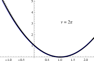
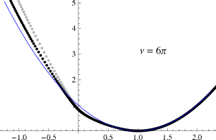
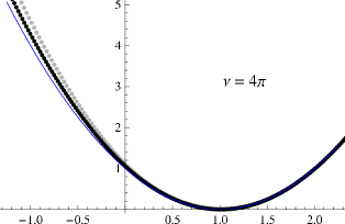
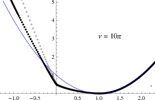
Figure 6: Behaviour of the large deviation function as a function of the current $j/(\nu\rho(1-\rho))$ for different values of $\nu$. The gray dots correspond to $L=50,N=25$ and the black dots correspond to $L=100,N=50$. They are obtained by solving numerically the functional Bethe Ansatz equation (47). The thin blue curve represents the leading Gaussian behaviour (50).

IV Multispecies exclusion processes and Matrix Ansatz

From the mathematical point of view, the ASEP is one of the simplest but non-trivial model for which the hydrodynamic limit can be rigorously proved. At large scales, the distribution of the particles of the ASEP emerges as a density field that evolves according to Burgers equation with a vanishingly small viscosity Spohn . The Burgers equation is the textbook prototype for shock formation: a smooth initial distribution can develop a singularity (a discontinuity) in finite time. A natural question that arises is whether this shock is an artifact of the hydrodynamic limit or whether, under some specific conditions, the original ASEP does display some singularity at the microscopic scale Andjel ; Ferrari ; Barma2 ; MartinSchock ; Janowski ; km . The question was answered positively: an abrupt transition does exist at the level of the particle system and its width is of the order of the lattice size. However, defining precisely the position of the shock at the microscopic level requires some thought, and this was achieved by introducing a second-class particle (see e.g., P. A. Ferrari, 1992 Ferrari ). This second class particle behaves as a first-class particle with respect to holes and as a hole with respect to first-class particles. The dynamical rules thus take the following form: $10\to 01\,\,\,\,12\to 21\,\,\,\,\hbox{ and }\,\,\,20\to 02\,,$ where all transitions occur with rate 1. This dynamics corresponds to coupling two TASEP models. In order to locate the shock it is enough to introduce a single second class particle in the system.

A straightforward generalization of the two species case of first and second class particles is the multispecies process where there is a hierarchy amongst the different species: first class particles have highest priority and can overtake all other classes of particles; second class particles can overtake all other classes except the first class etc… hence, during an infinitesimal time step $dt$, the following processes take place on each bond with probability $dt$:

$$I\ 0\to 0\ I \qquad\mbox{for}\quad I\neq 0$$

$$I\ J\to J\ I \qquad\mbox{for}\quad 1\leq I<J\leq N\,.$$ (51)

Note that particles can always overtake holes (= 0-th class particles). This model will be called the $N$-TASEP and it can be obtained by coupling $N$ ordinary TASEP models Liggett1 ; Liggett2 .

Suppose that there are $P_{I}$ particles of class $I$ on a ring of size $L$. Then, the total number of configurations is given by

$$\Omega=\frac{L!}{P_{0}!P_{1}!P_{2}!\ldots P_{N}!}$$

The total number of particles is given $P_{1}+\ldots P_{N}$. We warn the reader that in this section $N$ denotes the number of species and not the number of particles.

The object of this section is to provide an algebraic description of the stationary measure of this system.

IV.1 Matrix Ansatz for Two Species

The idea of representing the stationary weights of a configuration as traces over a quadratic algebra goes back to the seminal article of Derrida, Evans, Hakim and Pasquier in 1993 DEHP . These authors were studying the 1-species TASEP with open boundary conditions but they realized that the same idea could also be applied to the Two Species ASEP on a ring (Derrida, Janowski, Lebowitz and Speer, 1993 DJLS ). This technique, known as the Matrix Product Representation (or Matrix Ansatz), has been exceptionally fruitful in the field of one-dimensional stochastic models and has led to a very large number of exact solutions. This method seems to be complementary to the Bethe Ansatz in many problems and the exact relations between the two techniques is not yet fully understood Alcaraz2 ; ogkmMP . A solver’s guide to the Matrix Ansatz method has recently been written by R.A. Blythe and M. R. Evans MartinRev2 and contains many applications to various models.

Here, we explain how the Matrix Ansatz works for the two species TASEP on a ring, with dynamical rules given by (51). A Configuration of the model can be represented by a string made from the ’letters’ 1,2 and 0, e.g., ${\mathcal{C}}={0}{1}{22}{0}{2}{11}$. According to the Matrix Ansatz, the stationary weight of ${\mathcal{C}}$ is given by

$$P({\mathcal{C}})=P({0}{1}{22}{0}{2}{11})=\frac{1}{Z}{\rm Tr}({E}{D}{AA}{E}{A}{DD})\,,$$ (52)

where the string corresponding to ${\mathcal{C}}$ has been rewritten using the alphabet $D,A$ and $E$ through the correspondence: ${0}~{}\rightarrow~{}{E},$ ${1}~{}\rightarrow~{}{D}$ and ${2}~{}\rightarrow~{}{A}$. Here $D,A$ and $E$ are operators (matrices) which are in general non-commuting; we suppose that the Trace operation is well-defined on any product that contains at least one operator of each type. If the particles were totally independent then the stationary measure would be factorized and the probability of having a 0,1 or 2 at a site will be equal, respectively, to the density $\rho_{0}$ of holes, $\rho_{1}$ of 1’s or $\rho_{2}$ of 2’s. Of course, this is not true: the particles are strongly correlated by the dynamics. The Matrix Product Representation can be ‘justified’ a posteriori in an informal way by saying that in this Ansatz the stationary measure remains somehow factorized but correlations are taken into account because the operators $D,A$ and $E$ do not commute. As usual, the factor $Z$ in equation (52) is a normalization factor.

The operators $D,A$ and $E$ have to be chosen adequately so that the Ansatz (52) corresponds to the zero-eigenvector of the Markov matrix. It can be shown that the right choice in the case of the 2-TASEP model on a ring is obtained when these operators satisfy the following relations:

$${D}{E} = {D}+{E}\,,$$ (53)

$${D}{A} = {A}\,,$$ (54)

$${A}{E} = {A}\,.$$ (55)

The operators $D,A$ and $E$ thus define a quadratic algebra. These algebraic rules are enough to allow the computation of the steady state probability of any configuration. For example,

$$P({0}{1}{22}{0}{2}{11})=\frac{1}{Z}{\rm Tr}(D^{2}EA^{3})=\frac{1}{Z}{\rm Tr}((D^{2}+D+E)A^{3})=3\frac{1}{Z}{\rm Tr}(A^{3}).$$

The overall normalization constant can also be determined. It is possible to prove from algebraic relations (53, 54, 55) that the weights defined by the Matrix Ansatz correspond to the stationary probabilities. This Ansatz allows to calculate many stationary state properties such as currents, correlations, fluctuations DJLS . Besides, it can be shown, using Matrix Ansatz, that the stationary measure of the Two Species TASEP on a ring is not Gibbsean (Speer, 1993 Speer ).

The algebra (53, 54, 55) encodes combinatorial recursion relations between configurations corresponding to different system sizes. Although most of the calculations can be done just by using the abstract algebraic relations between $D$, $E$ and $A$ that define the algebra, it can be sometimes helpful to work with an explicit representation. The non-commuting representations of the algebra (53, 54, 55) are necessarily infinite dimensional. One of the most popular representation is the following:

$$D=\left(\begin{array}[]{ccccc}1&1&0&0&\dots\\ 0&1&1&0&\\ 0&0&1&1&\ddots\\ &&&\ddots&\ddots\end{array}\right),\,\,E=D^{\dagger},\,\,A=\left(\begin{array}[]{cccc}1&0&0&\dots\\ 0&0&0&\dots\\ 0&0&0&\dots\\ .&.&.&.\end{array}\right)\,\;$$ (64)

These matrices operate on an infinite dimensional space with countable basis. It we write $D=1+\delta$ and $E=1+\epsilon$, we note that ${\delta}$ corresponds the right-shift and $\epsilon$ to the left-shift. The operator $A$ is simply the projector on first coordinate. We also remark that any finite product of the matrices $D$, $E$ and $A$ that contains at least one $A$ is a finite rank matrix and thus has a finite trace.

Apart from an isolated attempt to solve the 3-TASEP using the Matrix Ansatz that did not seem to extend to higher class models MMR , no representation for the $N-$TASEP stationary measure was known until 2007. The breakthrough was made in the mathematical literature and came from a very different direction, queuing theory.

IV.2 Geometric interpretation of the 2-TASEP stationary measure

In FerrariMartin , P. A. Ferrari and J. B. Martin found an independent construction of the 2-TASEP steady state that does not rely on the Matrix Ansatz but rather on a queuing model interpretation. These authors construct a 2-TASEP configuration with $P_{1}$ First Class Particles and $P_{2}$ Second Class Particles starting from two independent configurations of the 1 species TASEP defined on two parallel lines.

One starts from a two-line configuration of particles (with at most one particle per site). The following algorithm will be easier to follow by looking at Figure 7 in which the construction in drawn step by step: On line 1 there are $P_{1}$ particles distributed randomly amongst the $L$ available sites. On line 2, there are $P_{1}+P_{2}$ particles also distributed randomly amongst the $L$ sites. Working from right to left we associate to each particle on line 1, the nearest particle, at the site just below it or to its left, on line 2 that has not been already associated to another particle. The particles in line 2 that are paired to particles on the first line are labeled 1; the $P_{2}$ particles on line 2 that remain unassociated are labeled 2. The empty sites of line 2 are labeled 0, thus each site of line 2 is labeled 0, 1 or 2. Hence, a configuration of the two species TASEP containing $P_{1}$ first-class and $P_{2}$ second-class particles is generated by the construction. Since we consider periodic boundary conditions, the site at which we begin this procedure will not affect the two species TASEP configuration that is obtained. The procedure is summarized in Figure 8.

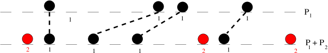
Figure 7: Step by step decomposition of the Ferrari and Martin construction.

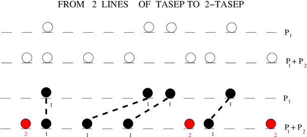
Figure 8: A synthetic view of the Ferrari and Martin construction: starting from two lines of TASEP with only one type of (colorless) particles, a 2-TASEP configuration is constructed with first class particles (in black), second class particles (in red) and holes (empty sites).

It is important to note that this construction is NOT one-to one: different configurations of the $P_{1}$ particles on line 1 can lead to the same final 2-TASEP configuration on line 2. The fundamental claim, proved in FerrariMartin , is the following: the weight of a 2-TASEP configuration is proportional to the total number of ways you can generate it by the Ferrari-Martin construction. By examining carefully the Figure 8, one can make the following fundamental observations:

• A particle 1 (on the 1st line) can not be located above a 2 on the 2nd line.

• Factorisation Property: All the 1’s (on the 2nd line) situated between two 2’s MUST be linked to 1’s (on the 1st line) that are located between the positions of the two 2’s (No Crossing Condition).

• ‘Pushing’ Procedure: The ‘ancestors’ of a string of the type $210102$ are the strings obtained by pushing the 1’s to the right i.e., $210102,210012,201102,201012,200112$.

In fact, these properties uniquely characterize the stationary weights. Furthermore, one can prove that the matrix Ansatz automatically performs the combinatorics underlying the geometrical construction of the weights. More precisely, one can construct in a systematic manner the quadratic algebra generated from $A,D$ and $E$ from the Ferrari-Martin procedure EFM ; reciprocally one can deduce this procedure from the algebra (53, 54, 55). This correspondence leads to the following properties:

• The Factorisation Property is related to the fact that $A$ is a PROJECTOR.

• The Pushing Procedure leads to the fact that$D$ and $E$ are SHIFT OPERATORS (right-shift and left-shift, respectively).

IV.3 Solution of the $N$-TASEP

The geometric construction of Ferrari-Martin was carried out recursively to the $N$-TASEP model FerrariMartin . In Figure 9, the 3-TASEP is described: one starts with 3 lines of the 1-TASEP, containing respectively $P_{1}$, $P_{1}+P_{2}$ and $P_{1}+P_{2}+P_{3}$ particles with no labels. All the $P_{1}$ particles on the first line are in black and considered to be 1st-class particles. One starts by pairing from right to left the 1st-class particles from the 1st line to the 2nd line. This procedure is repeated from the 2nd line to the 3rd line on so on. Each line has thus $P_{1}$ 1st-class particles, in black. These 1st-class particles are now considered to be spectators. The $P_{2}$ unselected particles on the second line are 2nd-class particles, they are colored in red. We associate the $P_{2}$ red-particles of the second line to $P_{2}$ particles on the third line again from right to left. Now on the third line, we have $P_{1}$ 1st-class particles (in black), $P_{2}$ 2nd-class particles (in red), and the remaining, unselected, $P_{3}$ particles are 3rd-class particles (in blue). We have thus constructed a 3-TASEP configuration on the third line. This method extends to the $N$-TASEP in a natural manner (for a precise description see FerrariMartin ; EFM ).

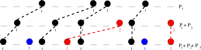
Figure 9: The Ferrari and Martin construction for the 3-TASEP . On the last line, a 3-TASEP configuration is generated with first class particles (in black), second class particles (in red) third class particles (in blue) and holes (empty sites).

Here again, the same 3-TASEP configuration on the third line can be generated in different ways. The weight of a 3-TASEP configuration is proportional to the total number of ways you can generate it by this construction. The Matrix Ansatz for the 3-TASEP is the algebraic counterpart of this procedure. It was shown in EFM that the recursive geometrical construction leads to a hierarchical definition of the operators $\hat{\bf P}_{0},\hat{\bf P}_{1},\hat{\bf P}_{2}$ and $\hat{\bf P}_{3}$ corresponding to the particles $0,1,2,$ and 3 based onTensor Products of elements of the original quadratic algebra. Indeed, for the 3-TASEP case, we find using $D$, $A$ and $E$ matrices and the shift operators $\delta=D-1$ and $\epsilon=E-1$:

$$\hat{\bf P}_{0} = {\bf 1}\otimes{\bf 1}\otimes E+{\bf 1}\otimes\epsilon\otimes A+\epsilon\otimes{\bf 1}\otimes D\,.$$ (65)

$$\hat{\bf P}_{1} = {\bf 1}\otimes{\bf 1}\otimes D+\delta\otimes\epsilon\otimes A+\delta\otimes{\bf 1}\otimes E$$ (66)

$$\hat{\bf P}_{2} = A\otimes{\bf 1}\otimes A+A\otimes\delta\otimes E$$ (67)

$$\hat{\bf P}_{3} = A\otimes A\otimes E$$ (68)

More generally, the Ferrari-Martin construction allows to construct a Matrix Ansatz for the $N$-TASEP and also provides an interpretation of the operators that appear in the Matrix Ansatz as priority queue matrices EFM .

We now discuss the case of the $N$-ASEP model. If backward jumps are allowed (rate $x\neq 0$), the $N$-ASEP dynamical rules are

$$JK\to KJ 1 1\leq J<K\leq N$$  with rate  if (69)

$$KJ\to JK x 1\leq J<K\leq N$$  with rate  if (70)

$$J0\to 0J 1 1\leq J\leq N$$  with rate  if (71)

$$0J\to J0 \mbox{\quad with rate $x$ \quad if $1\leq J\leq N$}\;.$$ (72)

Unfortunately, the Ferrari-Martin construction can not be generalized to the $N$-ASEP model. This can be understood by the fact that the procedure for the TASEP is local and directed (a particle is associated with the nearest particle on its left in the next line) and by introducing backward jumps the queuing theory interpretation is lost. In fact it can be shown that no construction similar to that of Ferrari and Martin can exist for the $N$-ASEP and this method can not be used to determine the steady state measure of the $N$-ASEP on a ring.

However, using the operators defined in equations (65–68) and deforming the underlying quadratic algebra in the following manner:

$$DE-xED = (1-x)(D+E)$$ (73)

$$DA-xAD = (1-x)A$$ (74)

$$AE-xEA = (1-x)A\;,$$ (75)

we proved in PEM that the deformed tensor algebra solves the $N$-ASEP. We note that the shift-operators, still defined by $\delta=D-1$ and $\epsilon=E-1$, satisfy the $x$-deformed oscillator algebra:

$$\delta\epsilon-x\epsilon\delta=1\,,$$

as can be shown using equation (73). In fact, a similar deformation method allows to find the steady state of the $N$-ASEP as proved in PEM .

To conclude, we emphasize that in the present problem, the Matrix Ansatz is not simply a reformulation of a known algorithm but it also plays a constructive role and allows to derive new results which are not accessible by other means. Besides, in the TASEP case, the Ferrari and Martin construction provides for the first time EFM an interpretation of the infinite-dimensional operators that appear in the Matrix Ansatz: the mapping to a queueing process provides a natural representation of the space on which the matrices act as counting operators (for an alternative interpretation of the Matrix Ansatz see Woelki ). There are many ways to generalize the TASEP to multispecies models (by introducing e.g. species-dependent switching rates, or open boundary conditions Ayyer ) and we believe that the algebraic deformation technique explained above can be adapted to various unsolved problems. The $N$-ASEP also displays remarkable properties that have been investigated by combinatorial methods Chikashi and partially by the Bethe Ansatz for $N=2$ Cantini ; evans ; Wehefritz but many open problems remain to be solved.

V Conclusion

The asymmetric exclusion process seems deceptively simple and the incredible number and complexity of the studies that it stimulated appears totally incredible. Such a wonder seems to defy explanation. Very few models have met such a rare success: one example that comes to mind is the Ising model.

The present article stems from a talk given at STATPHYS24 and discusses some recent works. It does not pretend to be an exhaustive review. We focused on models on a finite periodic lattice that we analyzed by two techniques, the Bethe Ansatz and the matrix product representation. The bibliography, although quite substantial, reflects this subjective choice. The ASEP can be investigated through a huge variety of techniques: Bethe Ansatz, Quadratic Algebras, Young tableaux, Combinatorics, Orthogonal polynomials, Random Matrices, Stochastic differential equations, determinantal representations, hydrodynamic limits etc. Each of these approaches is becoming a specific subfield that has its own links with other branches of theoretical physics and mathematics. We refer the reader who wishes to broaden his (her) perspective to recent review articles and to other contributions to this special issue. In particular, the ASEP on the infinite lattice, the relations with random matrix theory and the recently derived exact results for the Kardar-Parisi-Zhang equation in one dimension, are reviewed in the articles of P. L. Ferrari and of H. Spohn and T. Sasamoto.

I am grateful to my colleagues, C. Arita, A. Ayyer, M. Evans, P. Ferrari, O. Golinelli, S. Prolhac, N. Rajewski and M. Woelki, with whom I had the pleasure to work on the subjects presented here during the last years. I thank S. Mallick for collaboration and for his careful reading of the manuscript.

References

- (1) G. Albertini, S. R. Dahmen, B. Wehefritz, 1997, The free energy singularity of the asymmetric 6-vertex model and the excitations of the asymmetric XXZ chain, Nucl. Phys. B 493 541.
- (2) F. C. Alcaraz, M. Droz, M. Henkel, V. Rittenberg, 1994, Reaction-diffusion processes, critical dynamics and quantum chains, Ann. Phys. 230, 250.
- (3) F. C. Alcaraz and M. J. Lazo, 2004, The Bethe ansatz as a matrix product ansatz, J. Phys. A: Math. Gen. 37, L1.
- (4) F. C. Alcaraz and V. Rittenberg, 2007, Different facets of the raise and peel model, J. Stat. Mech.: Theor. Exp. P07009.
- (5) E. D. Andjel, M. Bramson and T. M. Liggett, 1988, Shocks in the asymmetric simple exclusion process, Prob. Theor. Rel. Fields 78, 231.
- (6) C. Appert-Rolland, B. Derrida, V. Lecomte and F. Van Wijland, 2008, Universal cumulants of the current in diffusive systems on a ring, Phys. Rev. E 78, 021122.
- (7) A. Ayyer, J. L. Lebowitz and E. R. Speer, 2009, On the two species asymmetric exclusion process with semi-permeable boundaries, J. Stat. Phys. 135, 1009.
- (8) M. Barma, 1992, Dynamics of field-driven interfaces in the two-dimensional Ising model, J. Phys. A: Math. Gen 25, L693.
- (9) R. J. Baxter, 1982 Exactly solvable models in Statistical Mechanics (Academic Press, San Diego).
- (10) R. J. Baxter, 2002, Completeness of the Bethe Ansatz for the six and eight-vertex models, J. Stat. Phys. 108, 1.
- (11) H. Bethe, 1931, Zur Theory der Metalle. I Eigenwerte und Eigenfunctionen Atomkette Zur Physik 71, 205.
- (12) R. A. Blythe and M. R. Evans, 2007, Nonequilibrium steady states of matrix-product form: a solver’s guide, J. Phys. A: Math. Theor. 40, R333.
- (13) N. M. Bogoliubov, 2009, Determinantal representation of correlation functions in the totally asymmetric exclusion model, SIGMA 5, 052 (arXiv:0904.3680).
- (14) T. Chou and D. Lohse, 1999, Entropy-driven pumping in zeolites and biological channels, Phys. Rev. Lett. 82, 3552.
- (15) C. Arita, A. Kuniba, K. Sakai and T. Sawabe, 2009 Spectrum of a multi-species asymmetric simple exclusion process on a ring, J. Phys. A: Math. Theor. 42, 345002.
- (16) L. Bertini, A. De Sole, D. Gabrielli, G. Jona-Lasinio and C. Landim, 2002, Macroscopic Fluctuation Theory for stationary non-equilibrium states, J. Stat. Phys. 107, 635.
- (17) T. Bodineau, B. Derrida, 2005, Distribution of currents in non-equilibrium diffusive systems and phase transitions, Phys. Rev. E 72, 066110.
- (18) T. Bodineau, B. Derrida, 2007, Cumulants and large deviations of the current through non-equilibrium steady states, C. R. Physique 8, 540.
- (19) S. Chatterjee and M. Barma, 2008, Shock probes in a one-dimensional Katz-Lebowitz-Spohn model, Phys. Rev. E 77, 061124.
- (20) L. Cantini, 2008, Algebraic Bethe Ansatz for the two-species ASEP with different hopping rates, J. Phys. A: Math. Theor. 41, 095001.
- (21) J. de Gier, F. H. L. Essler, 2005, Bethe Ansatz solution of the Asymmetric Exclusion Process with Open Boundaries, Phys. Rev. Lett. 95, 240601.
- (22) J. de Gier and F. H. F. Essler, 2006, Exact spectral gaps of the asymmetric exclusion process with open boundaries, J. Stat. Mech.: Theor. Exp. P12011.
- (23) J. de Gier and F. H. F. Essler, 2008, Slowest relaxation mode of the partially asymmetric exclusion process with open boundaries, J. Phys. A: Math. Theor. 41, 485002.
- (24) B. Derrida, 1998, An exactly soluble non-equilibrium system: the asymmetric simple exclusion process, Phys. Rep. 301, 65.
- (25) B. Derrida, 2007, Non-equilibrium steady states: fluctuations and large deviations of the density and of the current, J. Stat. Mech.: Theor. Exp. P07023.
- (26) B. Derrida, M. R. Evans, 1999, Bethe Ansatz solution for a defect particle in the asymmetric exclusion process, J. Phys. A: Math. Gen. 32, 4833.
- (27) B. Derrida, M. R. Evans, V. Hakim, V. Pasquier, 1993, Exact solution of a 1D asymmetric exclusion model using a matrix formulation, J. Phys. A: Math. Gen. 26, 1493.
- (28) B. Derrida, S.A. Janowski, J. L. Lebowitz and E. R. Speer, 1993, Exact solution of the totally asymmetric exclusion process: shock profiles, J. Stat. Phys. 73, 813.
- (29) B. Derrida, J. L. Lebowitz, 1998, Exact large deviation function in the asymmetric exclusion process, Phys. Rev. Lett. 80, 209.
- (30) B. Derrida, K. Mallick, 1997, Exact diffusion constant for the one-dimensional partially asymmetric exclusion process, J. Phys. A: Math. Gen. 30, 1031.
- (31) D. Dhar, 1987, An exactly solved model for interfacial growth, Phase Transitions 9, 51.
- (32) T. C. Dorlas, A. M. Povolotsky and V. B. Priezzhev, 2009, From Vicious walkers to TASEP, J. Stat. Phys. 135, 483.
- (33) M. R. Evans, R. A. Blythe, 2002, Non-equilibrium dynamics in low dimensional systems, Physica A, 313, 110.
- (34) M. R. Evans, 1996, Bose-Einstein condensation in disordered exclusion models and relation to traffic flow, Europhys. Lett. 36, 13.
- (35) M. R. Evans, P. A. Ferrari and K. Mallick, 2009, Matrix Representation of the Stationary Measure for the Multispecies TASEP, J. Stat. Phys. 135, 217.
- (36) M. R. Evans, R. Juhàsz and L. Santen, 2003, Shock formation in an exclusion process with creation and annihilation, Phys. Rev. E 68, 026117.
- (37) P. A. Ferrari, 1992, Shock fluctuations in the asymmetric simple exclusion, Prob. Theor. Rel. Fields 91, 81.
- (38) P. A. Ferrari, L. R. G. Fontes, 1994, Current fluctuations for the asymmetric exclusion process, Ann. Prob. 22, 1.
- (39) P. A. Ferrari and J. B. Martin, 2007, Stationary distributions of multi-type totally asymmetric exclusion processes, Ann. Probab. 35, 807.
- (40) P. L. Ferrari, 2010, From Interacting particle systems to random matrices, arXiv:1008.4853.
- (41) C. Flindt, T. Novotný and A.-P. Jauho, 2004, Current noise in vibrating quantum array, Phys. Rev. B 70, 205334.
- (42) G. Gallavotti, E. G. D. Cohen, 1995 Dynamical ensembles in non-equilibrium statistical mechanics, Phys. Rev. Lett. 74, 2694.
- (43) F.R. Gantmacher, 1964, Matrix theory, (Chelsea, New York)
- (44) O. Golinelli, K. Mallick, 2005, Spectral gap of the totally asymmetric exclusion process at arbitrary filling, J. Phys. A: Math. Gen. 38, 1419.
- (45) O. Golinelli, K. Mallick, 2005 Spectral Degeneracies in the Totally Asymmetric Exclusion Process, J. Stat. Phys 120, 779.
- (46) O. Golinelli, K. Mallick, 2006, The asymmetric simple exclusion process : an integrable model for non-equilibrium statistical mechanics, J. Phys. A: Math. Gen. 39, 12679.
- (47) O. Golinelli and K. Mallick, 2006, Derivation of a matrix product representation for the asymmetric exclusion process from Algebraic Bethe Ansatz, J. Phys. A: Math. Gen. 39, 10647.
- (48) L.-H. Gwa, H. Spohn, 1992, Bethe solution for the dynamical-scaling exponent of the noisy Burgers equation, Phys. Rev. A 46, 844.
- (49) T. Halpin-Healy, Y.-C. Zhang, 1995, Kinetic roughening phenomena, stochastic growth, directed polymers and all that, Phys. Rep. 254, 215.
- (50) T. E. Harris, 1965, Diffusion with ‘collisions’ between particles, J. Appl. Prob. 2, 323.
- (51) S. A. Janowski, J. L. Lebowitz, 1992 Finite size effects and Shock fluctuations in the asymmetric exclusion process, Phys. Rev. A 45, 618.
- (52) C. Jarzynski, 1997, Nonequilibrium Equality for Free Energy Differences, Phys. Rev. Lett. 78, 2690.
- (53) K. Johansson, 2000, Shape fluctuation and random matrices, Comm. Math. Phys. 209, 437.
- (54) D. Kandel, E. Domany, B. Nienhuis, 1990, A six-vertex model as a diffusion problem: derivation of correlation functions, J. Phys. A: Math. Gen. 23, L755.
- (55) S. Katz, J. L. Lebowitz, H. Spohn, 1984, Nonequilibrium steady states of stochastic lattice gas models of fast ionic conductors, J. Stat. Phys. 34, 497.
- (56) P. L. Krapivsky, S. Redner and E. Ben-Naim, 2010, A Kinetic View of Statistical Physics (Cambridge: Cambridge University Press).
- (57) J. Krug, 1991, Boundary-induced phase transitions in driven diffusive systems, Phys. Rev. Lett. 67, 1882.
- (58) T. Kriecherbauer and J. Krug, 2010, A pedestrian’s view on interacting particle systems, KPZ universality and random matrices, J. Phys. A: Math. Theor. 43, 403001.
- (59) D. S. Lee, D. Kim, 1999, Large deviation function of the partially asymmetric exclusion process, Phys. Rev. E 59, 6476.
- (60) D. Kim, 1995, Bethe Ansatz solution for crossover scaling functions of the asymmetric XXZ chain and the Kardar-Parisi-Zhang-type growth model, Phys. Rev. E 52, 3512.
- (61) D. Kim, 1997, Asymmetric XXZ chain at the antiferromagnetic transition: spectra and partition functions, J. Phys. A: Math. Gen. 30, 3817.
- (62) R. P. Langlands and Y. Saint-Aubin, 1995, Algebro-geometric aspects of the Bethe equations in Strings and Symmetries, Lecture Notes in Physics, Vol. 447, (Springer)
- (63) J. L. Lebowitz, H. Spohn, 1999 A Gallavotti-Cohen type symmetry in the large deviation functional for stochastic dynamics, J. Stat. Phys. 95, 333.
- (64) T. M. Liggett, 1985, Interacting Particle Systems, (Springer-Verlag, New-York).
- (65) T. M. Liggett, 1999, Stochastic Models of Interacting Systems:Contact, Voter and Exclusion Processes, (Springer-Verlag, New-York).
- (66) S. N. Majumdar and M. Barma,1991, Tag diffusion in driven systems, growing interfaces, and anomalous fluctuations, Phys. Rev. B 44, 5306.
- (67) C. T. MacDonald, J. H. Gibbs, A. C. Pipkin, 1968, Kinetics of biopolymerization on nucleic acid templates, Biopolymers 6, 1.
- (68) C. T. MacDonald, J. H. Gibbs, 1969, Concerning the kinetics of polypeptide synthesis on polyribosomes, Biopolymers 7, 707.
- (69) K. Mallick, 1996, Shocks in the asymmetric exclusion model with an impurity, J. Phys. A: Math. Gen. 29, 5375.
- (70) K. Mallick, S. Mallick and N. Rajewski, 1999, Exact solution of an exclusion process with three classes of particles and vacancies, J. Phys. A: Math. Gen. 32, 8399.
- (71) A. M. Povolotsky, 2004, Bethe ansatz solution of zero-range process with non-uniform stationary state, Phys. Rev. E 69, 061109.
- (72) V. B. Priezzhev, 2003, Exact Nonstationary Probabilities in the Asymmetric Exclusion Process on a Ring, Phys. Rev. Lett. 91, 050601.
- (73) V. B. Priezzhev 2005, Non-stationary Probabilities for the asymmetric exclusion process on a ring, Pramana J. Phys. 64, 915.
- (74) V. B. Priezzhev and G. M. Schütz, 2008, Exact solution of the Bernoulli matching model of sequence alignment, J. Stat. Mech.: Theor. Exp. P09007.
- (75) S. Prolhac and K. Mallick, 2008, Current fluctuations in the exclusion process and Bethe Ansatz, J. Phys. A: Math. Theor. 41, 175002.
- (76) S. Prolhac, 2008, Fluctuations and skewness of the current in the partially asymmetric exclusion process, J. Phys. A: Math. Theor. 41, 365003.
- (77) S. Prolhac and K. Mallick, 2009, Cumulants of the current in a weakly asymmetric exclusion process, J. Phys. A: Math. Theor. 42, 175001.
- (78) S. Prolhac, 2010, Tree structures for the current fluctuations in the exclusion process, J. Phys. A: Math. Theor. 43, 105002.
- (79) S. Prolhac, M. R. Evans, K. Mallick, 2009, The matrix product solution of the multispecies partially asymmetric exclusion process, J. Phys. A: Math. Theor. 42, 165004.
- (80) R. Rajesh, D. Dhar, 1998, An exactly solvable anisotropic directed percolation model in three dimensions, Phys. Rev. Lett. 81, 1646.
- (81) B. Schmittmann and R. K. P. Zia, 1995, Statistical mechanics of driven diffusive systems, in Phase Transitions and Critical Phenomena vol 17., C. Domb and J. L. Lebowitz Ed., (San Diego, Academic Press).
- (82) F. Reif, 1965 Statistical Mechanics, Berkeley Physics Course Volume V, (Mc Graw Hill).
- (83) A. Schadschneider, 2001, Statistical mechanics of traffic flow, Physica A 285, 101.
- (84) A. Rakos and G. M. Schütz, 2005, Current distribution and random matrix ensembles for an integrable asymmetric fragmentation process, J. Stat. Phys. 118, 511.
- (85) G. M. Schütz, 1997, Exact solution of the master equation of the asymmetric exclusion process, J. Stat. Phys. 88, 427.
- (86) G. M. Schütz, 2001, Exactly Solvable Models for Many-Body Systems Far from Equilibrium in Phase Transitions and Critical Phenomena vol 19., C. Domb and J. L. Lebowitz Ed., (Academic Press, San Diego).
- (87) E. R. Speer, 1993, The two species totally asymmetric exclusion process, in Micro, Meso and Macroscopic approaches in Physics, M. Fannes C. Maes and A. Verbeure Ed. NATO Workshop ’On three levels’, Leuven, July 1993.
- (88) F. Spitzer, 1970, Interaction of Markov Processes, Adv. in Math. 5, 246.
- (89) H. Spohn, 2005, KPZ equation in one dimension and line ensembles, Pramana J. Phys. 64, 1.
- (90) H. Spohn, 2005, Exact solutions for KPZ-type growth processes, random matrices, and equilibrium shapes of crystals, in Fundamental Problems in Statistical Mechanics XI, Leuven, Sept. 2005, ArXiv:cond-mat/0512011.
- (91) H. Spohn, 1991, Large scale dynamics of interacting particles, (Springer-Verlag, New-York).
- (92) T. Sasamoto, 2007, Fluctuations of the one-dimensional asymmetric exclusion process using random matrix techniques, J. Stat. Mech.: Theor. Exp. P07007.
- (93) H. Touchette, 2009, The large deviation approach to statistical mechanics, Phys. Rep. 478 1.
- (94) C. A. Tracy and H. Widom, 1994, Level-Spacing distributions and Airy kernel, Comm. Math. Phys. 159, 151
- (95) C. A. Tracy and H. Widom, 2008, Integral Formulas for the Asymmetric Simple Exclusion Process, Comm. Math. Phys. 279, 815.
- (96) C. A. Tracy and H. Widom, 2008, A Fredholm determinant representation in ASEP, J. Stat. Phys. 132, 291.
- (97) C. A. Tracy and H. Widom, 2009, Asymptotics in ASEP with step initial condition, Comm. Math. Phys. 290, 129.
- (98) C. A. Tracy and H. Widom, 2009, Total current fluctuation in ASEP, J. Math. Phys. 50, 095204.
- (99) C. A. Tracy and H. Widom, 2010, Formulas for Joint Probabilities for the Asymmetric Simple Exclusion Process, J. Math. Phys. 51, 063302.
- (100) H. van Beijeren, R. Kutner and H. Spohn, 1985, Excess noise for driven diffusive systems, Phys. Rev. Lett. 54, 2026.
- (101) M. Gulácsi, H. van Beijeren, A. C. Levi, 1993, Phase diagram of the five-vertex model, Phys. Rev. E 47, 2473.
- (102) H. van Beijeren, 1991, Fluctuations in the motions of mass and of patterns in one-dimensional driven diffusive system, J. Stat. Phys. 63 47.
- (103) T. Karzig and F. von Oppen, 2010, Signatures of critical full counting statistics in a quantum-dot chain, Phys. Rev. B 81, 045317.
- (104) B. Wehefritz-Kaufmann, 2010, Dynamical critical exponent for Two-Species Totally Asymmetric Diffusion on a Ring, Proceedings of the XVIIIth International Colloquium on Integrable Systems and Quantum Symmetries (Prague, June 2009), arXiv:1005.1988.
- (105) M. Woelki and K. Mallick, 2010, Transfer matrices for the totally asymmetric simple exclusion process, J. Phys. A: Math. Theor. 43, 185003
- (106) R. K. P. Zia and B. Schmittmann, 2006, A possible classification of nonequilibrium steady states, J. Phys. A: Math. Gen. 39, L407.
- (107) R. K. P. Zia and B. Schmittmann, 2007, Probability currents as principal characteristics in the statistical mechanics of non-equilibrium steady states, J. Stat. Mech.: Theor. Exp. P07012.