Superfluidity in atomic Fermi gases

Abstract

In a trapped atomic Fermi gas, one can tune continuously via a Feshbach resonance the effective pairing interaction between fermionic atoms from very weak to very strong. As a consequence, the low temperature superfluidity evolves continuously from the BCS type in the weak interaction limit to that of Bose-Einstein condensation in the strong pairing limit, exhibiting a BCS-BEC crossover. In this paper, we review recent experimental progress in atomic Fermi gases which elucidates the nature of the superfluid phase as the interaction is continuously tuned. Of particular interest is the intermediate or crossover regime where the $s$-wave scattering length diverges. We will present an intuitive pairing fluctuation theory, and show that this theory is in quantitative agreement with existing experiments in cold atomic Fermi gases.

1 Introduction

Ultracold atomic Fermi gases have been a very exciting, rapidly developing field, which has emerged within the past several years, bridging condensed matter and atomic, molecular and optical physics [1]. Using a Feshbach resonance in a magnetic field, one can tune the effective pairing interaction strength between fermionic atoms from very weak to very strong [2]. As the interaction strength varies, the nature of the low temperature superfluidity of these Fermi gases evolves continuously from the BCS type in the weak coupling limit to Bose-Einstein condensation (BEC) in the strong pairing limit, exhibiting a BCS-BEC crossover, which has been of great theoretical interest since 1960’s [3, 4, 5, 1]. Of particular interest is the unitary regime, where the $s$-wave scattering length diverges. This is a strongly correlated regime where no small parameter is available for perturbative expansions. It has been expected that this regime provides a prototype for studying both high $T_{c}$ superconductors and strongly interacting Fermi gases which are also of interest to nuclear and astro-physicists.

In this paper, we first review experimental progress in atomic Fermi gases, with an emphasis on recent radio frequency spectroscopy measurements. Then we will present a pairing fluctuation theory compare with experiment. We show that this theory successfully explain experimental measurements.

2 Experimental progress

The first theoretical study of BCS-BEC crossover dates back to 1960’s, although it did not get much attention until the seminal work of Leggett in 1980 on BCS-BEC crossover at zero temperature [4]. The discovery of high Tc superconductivity in 1986 gave a strong boost to the interest in BCS-BEC crossover [6, 7, 8, 9, 10, 1]. It was suggested that the unusual pseudogap phenomena in the cuprate superconductors might have to do with BCS-BEC crossover. Experimental efforts in this area fell far behind, because it had been difficult to find a system where the attractive pairing interaction is tunable. Thanks to the laser cooling and trapping technique in 1990’s, one is able to create “artificial” many-body systems of fermionic atoms in a laboratory. The existence of a Feshbach resonance in these Fermi gases makes it possible to tune the interaction strength.

For ease of control, the Feshbach resonances for the two widely studied species, ⁶Li and ⁴⁰K, are both very wide. The interaction in both cases are of the short-range, $s$-wave type. They are often taken to be a contact potential in theoretical treatments.

The first experimental realization of BCS-BEC crossover was achieved in 2004 by Jin and coworkers, [11, 12] and almost the same time by the Grimm group [13] and the Ketterle group [14]. Due to the difficulty in tuning temperature $T$, the Fermi gases were either in the superfluid or normal state at given interaction strength (or the magnetic detuning). Continuous variation of the system as a function of temperature was first realized by the Thomas group [15] at unitarity. In collaboration with the theory group at Chicago [16], Thomas et al [17] observed for the first time continuous phase transition from the normal to superfluid state in a unitary ⁶Li gas. One could argue, of course, that the vortex measurement of the Ketterle group provided the most definitive smoking gun for a superfluid state. [18]

Besides the interaction strength, another great tunability is population imbalance between the two fermionic species to be paired [19]. It adds a whole new dimension to the phase diagram and makes the physics much richer. It also generates interest [20] in possible observation of the Larkin-Ovchinnikov-Fulde-Ferrell (LOFF) state [21]. Experimental work in population imbalanced Fermi gases was pioneered by the Hulet group [22] and the Ketterle group [23]. Experiment in the extreme population imbalanced limit by the Ketterle group manifested [24] the importance of Hartree-like correlation effects besides BCS-type of pairing.

Unlike an electron system, it has been difficult to measure the excitation gap in the Fermi gas superfluid. Among all experimental techniques, Radio frequency (RF) spectroscopy [13] is arguably the most direct probe. Using a tunable RF field to excite one of the two pairing atoms from a lower hyperfine state (level 2) to a higher hyperfine level 3 which do not participate in pairing, a higher frequency will be needed if the atoms in level 2 are paired. Such a frequency shift (detuning) provides a good measure of the excitation gap. Previous measurement by Grimm and coworkers [13], and later repeated by the Ketterle group [24], was done in a momentum integrated fashion. At low $T$, the RF spectra displayed double-peak structure, with a sharp peak at zero detuning and a broad peak at positive detuning. This double-peak feature was nicely interpreted [25, 26] as transitions from unpaired atoms the trap edge (corresponding to the sharp peak) and from a distribution of paired atoms in the inner part of the trap (broad peak). However, doubt was cast about the origin of the two peaks as to whether they reflect pairing of bound state effects [24] or simply a result of trap inhomogeneity [27]. Recently, attention was also drawn to final state effects both theoretically [28, 29] and experimentally [24].

A big step in the RF technique was the recent momentum-resolved RF spectroscopy experiment in ⁴⁰K by the Jin group [30]. With momentum resolution, RF spectroscopy is equivalent to the angle-resolved photoemission spectroscopy (ARPES) for an electron system, In fact, it is cleaner than ARPES in that ARPES is only a two-dimensional probe, which is often plagued by the existence of surface states, surface contaminations, work function, and the complication of energy dispersion in the third dimension. In comparison, of course, the signal-to-noise ratio in a Fermi gas experiment is much lower, as limited by the (low) total number of atoms in the gas. although the trap inhomogeneity adds complication to the interpretation of the spectrum. Like ARPES, momentum-resolved RF spectroscopy measures the fermion spectral function, $A(\mathbf{k},\omega)$, which is of central importance in characterizing the system.

3 Theoretical Formalism

In this section, we now present a simple pairing fluctuation theory, which was first developed [10] to explain the pseudogap phenomena in high Tc superconductors. Fermi gases in the presence of a Feshbach resonance can be effectively described by a two-channel model [2]. It has now been known that the closed-channel fraction [31, 32] is very small for both ⁶Li and ⁴⁰K, throughout the BCS-BEC crossover. Therefore, for these systems, a one-channel model is often used as a good approximation, given by the grand canonical Hamiltonian

$$H-\sum_{\sigma}\mu_{\sigma}N_{\sigma}=\sum_{\mathbf{k},\sigma}(\epsilon_{\mathbf{k}}-\mu_{\sigma})a_{\mathbf{k},\sigma}^{\dagger}a_{\mathbf{k},\sigma}$$ (1)

$$+{}\sum_{\bf q,k,k^{\prime}}U(\mathbf{k,k^{\prime}})a^{\dagger}_{\mathbf{q/2+k},\uparrow}a^{\dagger}_{\mathbf{q/2-k},\downarrow}a_{\mathbf{q/2-k^{\prime}},\downarrow}a_{\mathbf{q/2+k^{\prime}},\uparrow},$$

where $\epsilon_{\mathbf{k}}=\hbar^{2}k^{2}/2m$ is the free atom dispersion. The difference between Eq. (1) and its BCS counterpart is that BCS keeps only the $\mathbf{q}=0$ term in the interactions. The inclusion of finite $\mathbf{q}$ terms allows incoherent, finite momentum pairing. For clarity of presentation, we will take a contact potential, $U(\mathbf{k,k^{\prime}})=1$, and use a 4-momentum notation, $K=(\mathbf{k},i\omega_{n})$, $Q=(\mathbf{q},i\Omega_{l})$, $\sum_{K}=T\sum_{\mathbf{k}}\sum_{n}$, and set $\hbar=1$. Population imbalance can be described by $\mu_{\uparrow}\neq\mu_{\downarrow}$. However, here we will only present the equations for the case of equal spin mixture. Generalization to population imbalance can be found in Ref. [33].

We assume that (i) the fermionic self energy $\Sigma$ has a pairing origin, (ii) pairs can be either condensed or fluctuating with a finite momentum, and (iii) condensed and noncondensed pairs do not mix at the level of $T$-matrix approximation. Figure 1 shows diagrammatically the contributions to the self-energy, where the double (red) lines indicate finite momentum pairs and the dotted line indicates the condensate. The subscripts “sc” and “pg” stand for superfluid condensate and pseudogap contributions, respectively.

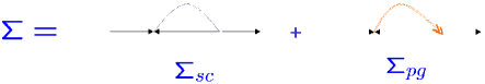
Figure 1: Schematic diagrams for the fermionic self-energy $\Sigma(K)$. The dotted and (red) double lines represent the condensate and finite momentum pairs, respectively.

To tackle this problem, we use a Green’s function method. We derive the equations of motion for one- and two-particle Green’s functions $G$ and $G_{2}$, which will involve higher order, three particle Green’s functions $G_{3}$: $i\dot{G}=[H,G]\sim G,G_{2}$, $i\dot{G}_{2}=[H,G_{2}]\sim G,G_{2},G_{3}$. We then truncate the equations of motion at the level of $G_{3}$, factorize $G_{3}$ into a sum of products of $G$ and $G_{2}$, and treat $G$ and $G_{2}$ on equal footing. For $G_{2}$, we focus on the particle-particle channel, neglecting the particle-hole channel which normally only provides a chemical potential shift. We emphasize that it is the particle-particle channel that gives rise to superfluidity. After some lengthy but straightforward derivation, we obtain the self energy:

$$\Sigma(K) = \Sigma_{sc}(K)+\Sigma_{pg}(K),$$ (2)

$$\Sigma_{sc}(K) = -\Delta_{sc}^{2}G_{0}(-K),$$ (3)

$$\Sigma_{pg}(K) = \sum_{Q}t_{pg}(Q)G_{0}(Q-K),$$ (4)

where

$$t_{pg}(Q)=\sum_{Q}\frac{U}{1+U\chi(Q)}$$ (5)

is the (pseudogap) $T$-matrix, and $\chi(Q)=\sum_{K}G_{0}(Q-K)G(K)$ is the pair susceptibility. Here $G_{0}$ is the bare Green’s function. A detailed derivation of this result can be found in Ref. [34]. Note that the $T$-matrix is effectively a renormalized pairing interaction. It shares exactly the same pole structure as the two-particle Green’s function, $G_{2}$. Through a Taylor expansion of its denominator, one can extract the pair dispersion:

$$t_{pg}^{-1}(Q)\approx Z(i\Omega_{l}-\Omega_{q}+\mu_{pair})\,.$$ (6)

The superfluid instability is given by $1+U\chi(0)=0\propto\mu_{pair}$, which is the BEC condition for pairs. Note that $\chi(Q)$ involves a mix of bare and full Green’s functions. We emphasize that this is a natural consequence of the equation of motion technique since it involves the operator $\hat{G}_{0}^{-1}$. It is this $G_{0}G$ form of $\chi$ that leads back to the BCS-form of gap equation in the absence of finite momentum pairs.

We focus on the superfluid phase where $t_{pg}(Q)$ diverges at $Q=0$. Defining

$$\Delta_{pg}^{2}\equiv-\sum_{Q\neq 0}t_{pg}(Q),$$ (7)

we have

$$\Sigma_{pg}(K) = -\left[\sum_{Q}t_{pg}(Q)\right]G_{0}(-K)+\delta\Sigma$$ (8)

$$= {}-\Delta_{pg}^{2}G_{0}(-K)+\delta\Sigma.$$

Neglecting the residue term $\delta\Sigma$, $\Sigma_{pg}$ takes the same form as $\Sigma_{sc}$. Thus we have immediately the BCS form of total self energy, $\Sigma(K)=-\Delta^{2}G_{0}(-K)$, with $\Delta^{2}=\Delta_{sc}^{2}+\Delta_{pg}^{2}$. This then leads to the BCS form of gap equation,

$$1+U\sum_{\mathbf{k}}\frac{1-2f(E_{\mathbf{k}})}{2E_{\mathbf{k}}}=0,$$ (9)

where $E_{\mathbf{k}}=\sqrt{(\epsilon_{\mathbf{k}}-\mu)^{2}+\Delta^{2}}$ is the quasiparticle dispersion. Different from the BCS mean-field theory, we emphasize that here $\Delta^{2}$ contains contributions from both condensed and noncondensed pairs so that it in general does not vanish at $T_{c}$. Note that the finite $\mathbf{q}$ pairs are different from the order parameter collective modes; the latter represent a coherent motion of the condensate. Here $\Delta_{sc}^{2}$ and $\Delta_{pg}^{2}$ are loosely proportional to the density of condensed and noncondensed pairs, respectively.

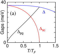
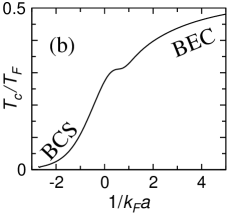
Figure 2: Typical behavior of (a) the temperature dependence of the gaps in a pseudogapped superfluid, and of (b) $T_{c}$ as a function of $1/k_{F}a$ in a trap, where $k_{F}$ is the noninteracting Fermi momentum, and $a$ is the $s$-wave scattering length.

Equations (9) and (7), along with the number equation

$$n=2\sum_{K}G(K),$$ (10)

form a closed set of equations for the homogeneous case, which can be used to solve for $\mu$, $T_{c}$, and the gaps at $T\leq T_{c}$. $T_{c}$ is determined by setting $\Delta_{sc}=0$. Typical behaviors of the gaps are shown in Fig. 2(a).

To address Fermi gases in a trap, we use the local density approximation, by replacing $\mu\rightarrow\mu-V_{trap}(r)$. Then the number equation becomes $N=\int d^{3}r\,n(r)$. In Fig. 2(b) we show the BCS-BEC crossover behavior of $T_{c}$ in a trap. Here $1/k_{F}a$ parametrizes the interaction strength.

The RF response can be derived using the linear response theory. The RF interaction is described by

$$H_{rf}=e^{i\Omega t}\int d^{3}x\,\psi_{3}^{\dagger}\psi_{2}+h.c.,$$ (11)

and the response Kernel by

$$D(i\Omega_{l})=\sum_{K}G^{(2)}(K)G^{(3)}(K+Q).$$ (12)

We assume hyperfine level 3 was initially empty. In the absence of final state interactions, as in ⁴⁰K, we obtain [35] the RF current

$$I(k,\nu) = -\frac{1}{\pi}\mbox{Im}\,D^{R}(\nu+\mu-\mu_{3})$$ (13)

$$= \left.\frac{1}{2\pi}\sum_{\mathbf{k}}A(\mathbf{k},\omega)f(\omega)\right|_{\omega=\epsilon_{\mathbf{k}}-\mu-\nu}.$$

In order to address $A(\mathbf{k},\omega)=-2\,\mbox{Im}\,G(\mathbf{k},\omega+i0^{+})$ properly, we need to include the lifetime effects of finite momentum pairs and add an incoherent term $i\Sigma_{0}$ in (and only in) $\Sigma_{pg}$, reflecting the residue term $\delta\Sigma$ which we drop in solving the set of equations, i.e.,

$$\Sigma_{pg}(\mathbf{k},\omega)=\frac{\Delta^{2}_{pg}}{\omega+\epsilon_{\mathbf{k}}-\mu+i\gamma}-i\Sigma_{0}.$$ (14)

While above $T_{c}$ the spectral function with a pseudogap constitute a double peak structure with suppressed spectral weight at the Fermi level, below $T_{c}$, there is a zero at $\omega=-(\epsilon_{\mathbf{k}}-\mu)$. As $\Delta_{sc}$ increases with decreasing $T$ below $T_{c}$, the spectral peaks sharpen rapidly. This is a phase coherence effect. The parameters $\gamma$ and $\Sigma_{0}$ can be estimated from experimental RF spectra.

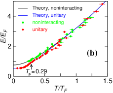
Figure 3: Comparison of (a) density profile and (b) energy $E/E_{F}$ for a unitary ⁶Li gas between theory (curves) and experiment (symbols). Also shown in (b) is comparison for the noninteracting energy. Here $E_{F}=k_{B}T_{F}$ is the noninteracting Fermi energy.

4 Comparison between theory and experiment

In Fig. 3, we compare between theory (curves) and experiment (symbols) (a) the density profile [36] and (b) system energy [17] for ⁶Li in the unitary limit. Both experimental and theoretical density profiles are very smooth, in good agreement with each other. Alternative theories predicts either a kink at the edge of the superfluid core or nonmonotonic radial and temperature dependence. The energy comparison also reveals a quantitative agreement. The fact that the unitary and noninteracting curves merge at $T\approx 0.6T_{F}\gg T_{c}$ manifests the presence of a pseudogap. It should be noted that there is no fitting parameter in our theoretical calculations.

Shown in Fig. 4 is a comparison of the spectral intensity map as a function of $k$ and single-particle energy $\omega+\mu$ between experiment [30] and theory [35] for a unitary ⁴⁰K gas at a temperature slightly above $T_{c}$. The white dashed curve is the experimentally extracted quasiparticle dispersion, whereas the solid curve is obtained theoretically following the experimental procedure. It is evident that theoretical and experimental results are rather close to each other. Indeed, as $T$ decreases from above to below $T_{c}$, the spectral intensity map evolves [35] from an upward dispersing branch at high $T$ to a bifurcation around $T_{c}$, and finally to a downward dispersing branch at $T\ll T_{c}$. This result establishes the actual single particle dispersions which contribute to the RF current, revealing that the broad peak in previous momentum-integrated RF spectra [13] indeed has a pairing origin. Furthermore, it also shows that, despite the trap inhomogeneity, momentum resolved RF spectroscopy can still provide a quantitative measure of the spectral function and single particle dispersion. It also lends support for the present $G_{0}G$ scheme since alternative NSR-based theories do not [37] seem to generate the two-branch-like feature observed in Ref. [30]. The downward dispersion around (and above) $T_{c}$ provides direct evidence for the existence of a pseudogap above $T_{c}$ at unitarity. Our theory serves as a basis for momentum-resolved RF spectroscopy analysis.

In summary, we have presented a pairing fluctuation theory where finite momentum pairing plays a progressively more important role as the pairing strength increases, leading to a pseudogap in the single particle excitation spectrum. This theory has been successfully applied to multiple experiments in atomic Fermi gases.

This work was supported by Zhejiang University and NSF of China Grant No. 10974173.

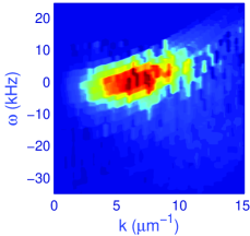
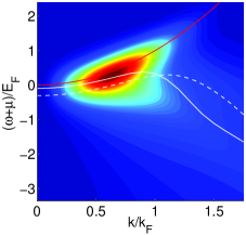
Figure 4: Comparison of spectral intensity map $I(k,\nu)k^{2}/(2\pi^{2})$ between experiment (left) from Ref. [30] and theory (right). The white dashed curve is an experimental extracted quasiparticle dispersion, and the white solid line is obtained theoretically following the same experimental data analysis procedure.

References

- [1] Q. J. Chen, J. Stajic, S. N. Tan, and K. Levin, Phys. Rep. 412, 1 (2005).
- [2] J. N. Milstein, S. J. J. M. F. Kokkelmans, and M. J. Holland, Phys. Rev. A 66, 043604 (2002).
- [3] D. M. Eagles, Phys. Rev. 186, 456 (1969).
- [4] A. J. Leggett, in Modern Trends in the Theory of Condensed Matter (Springer-Verlag, Berlin, 1980), pp. 13–27.
- [5] P. Nozières and S. Schmitt-Rink, J. Low Temp. Phys. 59, 195 (1985).
- [6] Y. J. Uemura, Physica C 282-287, 194 (1997).
- [7] R. Friedberg and T. D. Lee, Phys. Lett. A 138, 423 (1989).
- [8] Randeria, Physica B 198, 373 (1994).
- [9] B. Jankó, J. Maly, and K. Levin, Phys. Rev. B 56, R11407 (1997).
- [10] Q. J. Chen, I. Kosztin, B. Jankó, and K. Levin, Phys. Rev. Lett. 81, 4708 (1998).
- [11] C. A. Regal, M. Greiner, and D. S. Jin, Phys. Rev. Lett. 92, 040403 (2004).
- [12] Q. J. Chen, C. A. Regal, M. Greiner, D. S. Jin, and K. Levin, Phys. Rev. A73, 041601 (2006).
- [13] C. Chin, M. Bartenstein, A. Altmeyer, S. Riedl, S. Jochim, J. Hecker-Denschlag, and R. Grimm, Science 305, 1128 (2004).
- [14] M. W. Zwierlein, C. A. Stan, C. H. Schunck, S. M. F. Raupach, A. J. Kerman, andW. Ketterle, Phys. Rev. Lett. 92, 120403 (2004).
- [15] J. Kinast, A. Turlapov, and J. E. Thomas, arXiv:cond-mat/0409283.
- [16] Q. J. Chen, J. Stajic, and K. Levin, Phys. Rev. Lett.95, 260405 (2005).
- [17] J. Kinast, A. Turlapov, J. E. Thomas, Q. J. Chen, J. Stajic, and K. Levin, Science 307, 1296 (2005), published online 27 January 2005; doi:10.1126/science.1109220.
- [18] M. W. Zwierlein, J. R. Abo-Shaeer, A. Schirotzek, and W. Ketterle, Nature 435, 170404 (2005).
- [19] Q. J. Chen, Y. He, C.-C. Chien, and K. Levin, Phys. Rev. A 74, 063603 (2006).
- [20] Y. He, C.-C. Chien, Q. J. Chen, and K. Levin, Phys. Rev. A75, 021602(R) (2007).
- [21] P. Fulde and R. A. Ferrell, Phys. Rev. 135, A550 (1964); A. I. Larkin and Y. N. Ovchinnikov, Zh. Eksp. Teor. Fiz. 47, 1136 (1964) [Sov. Phys. JETP 20, 762 (1965)].
- [22] G. B. Partridge, W. Li, R. I. Kamar, Y. A. Liao, and R. G. Hulet, Science 311, 503 (2006).
- [23] M. W. Zwierlein, C. H. Schunck, A. Schirotzek, and W. Ketterle, Nature (London) 442, 54 (2006).
- [24] C. H. Schunck, Y. Shin, A. Schirotzek, M. W. Zwierlein, and W. Ketterle, Science 316, 867 (2007).
- [25] J. Kinnunen, M. Rodriguez, and P. Törmä, Science 305, 1131 (2004).
- [26] Y. He, Q. J. Chen, and K. Levin, Phys. Rev. A 72, 011602(R) (2005).
- [27] E. J. Mueller, arXiv:0711.0182 (unpublished).
- [28] S. Basu and E. Mueller, Phys. Rev. Lett. 101, 060405 (2008).
- [29] Y. He, C. C. Chien, Q. J. Chen, and K. Levin, Phys. Rev. Lett. 102, 020402 (2009).
- [30] J. T. Stewart, J. P. Gaebler, and D. S. Jin, Nature (London) 454, 744 (2008).
- [31] G. B. Partridge, K. E. Strecker, R. I. Kamar, M.W. Jack, and R. G. Hulet, Phys. Rev. Lett. 95, 020404 (2005).
- [32] Q. J. Chen and K. Levin, Phys. Rev. Lett. 95, 260406 (2005).
- [33] C.-C. Chien, Q. J. Chen, Y. He, and K. Levin, Phys. Rev. Lett. 97, 090402 (2006).
- [34] Q. J. Chen, Ph.D. thesis, University of Chicago, 2000, (available in the ProQuest Dissertations & Theses Database online).
- [35] Q. J. Chen and K. Levin, Phys. Rev. Lett. 102, 190402 (2009).
- [36] J. Stajic, Q. J. Chen, and K. Levin, Phys. Rev. Lett. 94, 060401 (2005).
- [37] E. Mueller, private communication.