Non-equilibrium dynamics in the quantum Brownian oscillator and the second law of thermodynamics

Abstract

We initially prepare a quantum linear oscillator weakly coupled to a bath in equilibrium at an arbitrary temperature. We disturb this system by varying a Hamiltonian parameter of the coupled oscillator, namely, either its spring constant or mass according to an arbitrary but pre-determined protocol in order to perform external work on it. We then derive a closed expression for the reduced density operator of the coupled oscillator along this non-equilibrium process as well as the exact expression pertaining to the corresponding quasi-static process. This immediately allows us to analytically discuss the second law of thermodynamics for non-equilibrium processes. Then we derive a Clausius inequality and obtain its validity supporting the second law, as a consistent generalization of the Clausius equality valid for the quasi-static counterpart, introduced in KIM10 .

1 Introduction

Over the past several decades there have been remarkable breakthroughs in experimental techniques for probing non-classical behaviors of small-scale quantum objects coupled to quantum environments (see, e.g., CAP05 ). Correspondingly, a more sophisticated theoretical understanding of the thermodynamic nature of such systems, especially in the low temperature regime where quantum effects are dominant, has been substantially demanded. In contrast to common quantum statistical mechanics, which is intrinsically based on a vanishingly small coupling between system and environment, the finite coupling strength between them in the quantum regime causes some subtleties that must be recognized.

At the heart of the aforesaid “quantum thermodynamics” MAH04 , the second law of thermodynamics, assumed to be inviolable by the scientific community for over a century CAL85 , has been confronted by challenges with considerable interest, and its absolute status has even come under increased scrutiny CAP05 ; MAH04 ; SHE02 . In fact, this fundamental law of nature has extensively been theoretically studied particularly in the scheme of a quantum harmonic oscillator linearly coupled to an independent-oscillator model of a heat bath (quantum Brownian oscillator) in equilibrium at a (low) temperature $T$, mainly due to its mathematical manageability.

A short overview of recent results either pro or contra the validity of the quantum second law has been given in KIM10 ; and the final result therein was that a properly defined Clausius inequality $\delta{\mathcal{Q}}_{\text{\scriptsize eff}}^{\star}\leq T_{\text{\scriptsize eff}}^{\star}\,dS_{N}$ representing the second law is valid without any previously argued violation in form of $\delta{\mathcal{Q}}\not\leq T\,dS$ at $T\to 0$. In the above inequality, $S_{N}$ represents the von-Neumann entropy of the coupled oscillator, which is, interestingly enough, identical to the thermal entropy of an uncoupled effective oscillator in equilibrium. And $\delta{\mathcal{Q}}_{\text{\scriptsize eff}}^{\star}$ is a heat exchanged between (weakly coupled) effective oscillator and bath, and $T_{\text{\scriptsize eff}}^{\star}$ a well-defined effective equilibrium temperature. This effective temperature differs from the temperature $T$ of the total system (oscillator plus bath) especially in the strong-coupling limit, where the total-system temperature is in fact not well-defined as an equilibrium temperature of the system oscillator since the reduced equilibrium density operator of the oscillator $\hat{H}_{s}$ is not any longer in form of the canonical thermal state $\hat{\rho}_{\beta}\propto e^{-\beta\hat{H}_{s}}$ with $\beta=1/(k_{B}\,T)$ KIM10 . This discrepancy between these two equilibrium temperatures is, of course, caused by the extra work (or energy) needed to couple an (uncoupled) oscillator to a bath COT11 . As a result, it may be legitimate to say that the original form of the Clausius inequality for the coupled oscillator in terms of the temperature $T$ is not well-defined rather than being violated.

However, the entire discussion of the quantum second law has so far been restricted to that for thermal equilibrium states, accordingly, in form of the Clausius equality. On the other hand, there has recently been an interesting result for a generalized Clausius inequality for non-equilibrium quantum processes, but restricted to isolated quantum systems (initially prepared at a thermal equilibrium state) LUT10 . In this paper we extend the above discussions into far-from-equilibrium processes in the scheme of quantum Brownian oscillator as a prototype of open quantum systems, but in the weak-coupling limit only since the exact treatment of the non-equilibrium processes in the strong-coupling limit is pretty much hopeless to leading to useful quantities in closed form to be needed for our discussion [cf. Eqs. (28)-(36)]. To do so, we consider the quantum oscillator with time-dependent Hamiltonian parameters, which finally enables us to derive a generalized Clausius inequality without any violation in variation of the Hamiltonian parameters as our central result. In fact, the time-dependent quantum oscillator has been studied by many authors for last about 60 years, initiated by Husimi HUS53 . In this paper we appeal to the method of quantum Liouville equation in order to directly obtain the time-dependent density operator of the system in consideration. This approach differs from that developed by Husimi, which is based on the fact that the Schrödinger equation for an isolated linear oscillator, rather than coupled to a bath, can reduce to a system of classical equations for the oscillator.

The general layout of this paper is the following. In Sect. 2 we review the general results of quantum Brownian oscillator needed for our later discussions. In Sect. 3 we consider non-equilibrium processes and then derive a closed expression for the time-dependent reduced density operator of the oscillator weakly coupled to a bath at an arbitrary time along the processes. In Sect. 4 the same discussion will take place for the corresponding quasi-static processes. Next the second law of thermodynamics for non-equilibrium processes will be systematically discussed in Sect. 5. Finally we give the concluding remarks of this paper in Sect. 6.

2 Basics of quantum Brownian oscillator

The quantum Brownian oscillator under investigation is described by the model Hamiltonian (Caldeira-Leggett model) WEI08 ; ING98

$$\hat{H}_{0}\;=\;\hat{H}_{s}\,+\,\hat{H}_{b}\,+\,\hat{H}_{sb}\,,$$ (1)

where a system linear oscillator, a bath, and a system-bath interaction are

$$\displaystyle\hat{H}_{s}\,=\,\frac{\hat{p}^{2}}{2M}+\frac{k_{0}}{2}\,\hat{q}^{2}\;\;\;;\;\;\;\hat{H}_{b}\,=\,\sum_{j=1}^{N}\left(\frac{\hat{p}_{j}^{2}}{2m_{j}}+\frac{k_{j}}{2}\,\hat{x}_{j}^{2}\right)$$ (2)

$$\displaystyle\hat{H}_{sb}\,=\,-\hat{q}\sum_{j=1}^{N}c_{j}\,\hat{x}_{j}\,+\,\hat{q}^{2}\sum_{j=1}^{N}\frac{c_{j}^{2}}{2\,k_{j}}\,,$$ (3)

respectively. Here the coupling strengths $c_{j}$, and the spring constants $k_{0}=M\omega_{0}^{2}$ and $k_{j}=m_{j}\omega_{j}^{2}$. The total system $\hat{H}_{0}$ is assumed to be within the canonical thermal equilibrium state $\hat{\rho}_{\beta}=e^{-\beta\hat{H}_{0}}/Z_{\beta}$, in form of a non-separable state ($\not\propto\hat{\rho}_{s}\otimes\hat{\rho}_{b}$) due to the interaction $\hat{H}_{sb}$, where the partition function $Z_{\beta}=\text{Tr}\,e^{-\beta\hat{H}_{0}}$. The second term of the interaction $\hat{H}_{sb}$, proportional to $\hat{q}^{2}$, was introduced in order to protect the pre-determined frequency ($\omega_{0}$) of the system oscillator $\hat{H}_{s}$ from its modification induced by the system-bath coupling (the first term linear in $\hat{x}_{j}$) WEI08 . Here the system and the bath effectively share the energy in the coupling term, especially in the strong-coupling limit ($c_{j}\gg 1$), and so it is in fact not completely clear whether this energy should be interpreted as belonging to the system or to the bath JAR04 . Therefore, without the above second term, the internal energy $U_{s}=\mbox{Tr}\,(\hat{H}_{s}\,\hat{\rho}_{\beta})$ of the coupled oscillator alone, with its unique frequency $\omega_{0}$, as well as its reduced density operator would not be well-defined [cf. Eqs. (59) and (65)]. In fact, from the Heisenberg equations of motion for $\hat{q}$ and $\hat{p}$ we can derive the quantum Langevin equation without the frequency shift as WEI08 ; ING98

$$M\,\ddot{\hat{q}}(t)\,+\,M\int_{0}^{t}d\tau\,\gamma(t-\tau)\,\dot{\hat{q}}(\tau)\,+\,M\omega_{0}^{2}\,\hat{q}(t)\;=\;\hat{\xi}(t)\,,$$ (4)

where the damping kernel and the noise operator are, respectively, given by

$$\gamma(t) = \frac{1}{M}\sum_{j=1}^{N}\frac{c_{j}^{2}}{m_{j}\,\omega_{j}^{2}}\,\cos(\omega_{j}\,t)$$ (5)

$$\hat{\xi}(t) = -M\gamma(t)\,\hat{q}(0)\,+\,\sum_{j=1}^{N}c_{j}\left\{\hat{x}_{j}(0)\,\cos(\omega_{j}\,t)\,+\,\frac{\hat{p}_{j}(0)}{m_{j}\,\omega_{j}}\,\sin(\omega_{j}\,t)\right\}\,.$$ (6)

Here as required, $\langle\hat{\xi}(t)\rangle_{\rho_{b^{\prime}}}=\text{Tr}\,\{\hat{\xi}(t)\,\hat{\rho}_{b^{\prime}}\}=0$, in which the shifted bath state $\hat{\rho}_{b^{\prime}}=e^{-\beta\,(\hat{H}_{b}+\hat{H}_{sb})}/Z^{(b^{\prime})}_{\beta}$ with the corresponding partition function $Z^{(b^{\prime})}_{\beta}$, and the noise correlation HAE05

$$\frac{1}{2}\left\langle\hat{\xi}(t)\,\hat{\xi}(t^{\prime})\,+\,\hat{\xi}(t^{\prime})\,\hat{\xi}(t)\right\rangle_{\rho_{b^{\prime}}}\,=\,\frac{\hbar}{2}\sum_{j=1}^{N}\frac{c_{j}^{2}}{m_{j}\,\omega_{j}}\cos\{\omega_{j}(t-t^{\prime})\}\,\coth\left(\frac{\beta\hbar\omega_{j}}{2}\right)\,.$$ (7)

Now we introduce a response function ING98

$$\chi_{AB}(t)\,=\,\frac{i}{\hbar}\,\left\langle[\hat{A}(t),\hat{B}(0)]\right\rangle_{\beta}\,\Theta(t)\,,$$ (8)

where $\Theta(t)$ represents a step function. Then it can easily be shown that $\chi_{pq}(t)=-\chi_{qp}(t)=M\dot{\chi}_{qq}(t)$ and $\chi_{pp}(t)=-M^{2}\ddot{\chi}_{qq}(t)$. For a later purpose it is also necessary to discuss the time-reversal dynamics of $\hat{q}(t)$ in terms of $\hat{r}(t):=\hat{q}(-t)$ and its momentum $\hat{s}(t):=-\hat{p}(-t)$. We can then derive the corresponding quantum Langevin equation HAE05

$$M\,\ddot{\hat{r}}(t)\,+\,M\int_{0}^{t}d\tau\,\gamma(t-\tau)\,\dot{\hat{r}}(\tau)\,+\,M\,\omega_{0}^{2}\,\hat{r}(t)\;=\;\hat{\xi}_{-}(t)\,.$$ (9)

While this is the same in form as Eq. (4), the two equations differ in the noise term in such a way that $\hat{\xi}_{-}(t)$ is identical to $\hat{\xi}(t)$, however, with replacement of $\hat{p}_{j}(0)\to-\hat{p}_{j}(0)$ in (6). From Eq. (8) and the stationarity relation $\langle\hat{A}(t)\,\hat{B}(0)\rangle_{\beta}=\langle\hat{A}(0)\,\hat{B}(-t)\rangle_{\beta}$ ING98 it appears as well that $\chi_{rr}(t)=-\chi_{qq}(t)$ and $\chi_{rs}(t)=-\chi_{rp}(t)=-\chi_{qp}(t)$ and $\chi_{ss}(t)=-\chi_{pp}(t)$. Applying the Laplace transform technique to Eqs. (4) and (9), respectively, we can finally obtain the exact expressions ILK10

$$\hat{q}(t) = -\chi_{qp}(t)\,\hat{q}+\chi_{qq}(t)\,\hat{p}-\sum_{j}\{\chi_{qp_{j}}(t)\,\hat{x}_{j}-\chi_{qx_{j}}(t)\,\hat{p}_{j}\}$$ (10a)

$$\hat{r}(t) = -\chi_{rp}(t)\,\hat{q}+\chi_{rr}(t)\,\hat{p}-\sum_{j}\{\chi_{rp_{j}}(t)\,\hat{x}_{j}-\chi_{rx_{j}}(t)\,\hat{p}_{j}\}\,,$$ (10b)

where the operators $\hat{q},\hat{p},\hat{x}_{j}$, and $\hat{p}_{j}$ represent the initial values $\hat{q}(0),\hat{p}(0),\hat{x}_{j}(0)$, and $\hat{p}_{j}(0)$, respectively. Here we have

$$\chi_{qx_{j}}(t)\,=\,\frac{1}{2\pi}\int_{-\infty}^{\infty}d\omega\,\tilde{\chi}_{qx_{j}}(\omega)\,e^{-i\omega t}$$ (11)

with $\tilde{\chi}_{qx_{j}}(\omega)=c_{j}/\{m_{j}\,(\omega_{j}^{2}-\omega^{2})\}\cdot\tilde{\chi}_{qq}(\omega)$, where the susceptibility $\tilde{\chi}_{qq}(\omega)$ is the the Fourier-Laplace transform of $\chi_{qq}(t)$. Also, $\chi_{rx_{j}}(t)=-\chi_{qx_{j}}(t)$, $\chi_{rp_{j}}(t)=\chi_{qp_{j}}(t)$, and $\chi_{qp_{j}}(t)=-m_{j}\,\dot{\chi}_{qx_{j}}(t)$.

It will also be useful later to introduce the well-known expressions for the equilibrium fluctuations in terms of the susceptibility $\tilde{\chi}_{qq}(\omega)$ such as FOR88

$$\langle\hat{q}^{2}\rangle_{\beta} = \frac{\hbar}{\pi}\int_{0}^{\infty}d\omega\,\coth\left(\frac{\beta\hbar\omega}{2}\right)\,\text{Im}\{\tilde{\chi}_{qq}(\omega+i\,0^{+})\}$$ (12a)

$$\langle\hat{p}^{2}\rangle_{\beta} = \frac{M^{2}\hbar}{\pi}\int_{0}^{\infty}d\omega\,\omega^{2}\,\coth\left(\frac{\beta\hbar\omega}{2}\right)\,\text{Im}\{\tilde{\chi}_{qq}(\omega+i\,0^{+})\}\,,$$ (12b)

which can be derived from the fluctuation-dissipation theorem CAL51 . For the Drude model (with a cut-off frequency $\omega_{d}$ and a damping parameter $\gamma_{o}$), which is a prototype for physically realistic damping, the equilibrium fluctuations are explicitly given by KIM07

$$\langle\hat{q}^{2}\rangle_{\beta}^{(d)} = \frac{1}{M}\sum_{l=1}^{3}\lambda_{d}^{(l)}\,\left\{\frac{1}{\beta\underline{\omega_{l}}}\,+\,\frac{\hbar}{\pi}\;\psi\left(\frac{\beta\hbar\underline{\omega_{l}}}{2\pi}\right)\right\}$$ (13)

$$\langle\hat{p}^{2}\rangle_{\beta}^{(d)} = -M\sum_{l=1}^{3}\lambda_{d}^{(l)}\,\underline{\omega_{l}}^{2}\,\left\{\frac{1}{\beta\underline{\omega_{l}}}\,+\,\frac{\hbar}{\pi}\;\psi\left(\frac{\beta\hbar\underline{\omega_{l}}}{2\pi}\right)\right\}\,,$$ (14)

respectively, where the digamma function $\psi(y)=d\,\ln\Gamma(y)/dy$ ABS74 , and $\underline{\omega_{1}}=\Omega$, $\underline{\omega_{2}}=z_{1}$, $\underline{\omega_{3}}=z_{2}$, and the coefficients

$$\lambda_{d}^{(1)}\;=\;\frac{z_{1}\,+\,z_{2}}{(\Omega\,-\,z_{1})(z_{2}\,-\,\Omega)}\;;\;\lambda_{d}^{(2)}\;=\;\frac{\Omega\,+\,z_{2}}{(z_{1}\,-\,\Omega)(z_{2}\,-\,z_{1})}\;;\;\lambda_{d}^{(3)}\;=\;\frac{\Omega\,+\,z_{1}}{(z_{2}\,-\,\Omega)(z_{1}\,-\,z_{2})}\,.$$ (15)

Here we have adopted, in place of $(\omega_{0},\omega_{d},\gamma_{o})$, the parameters $({\mathbf{w}}_{0},\Omega,\gamma)$ through the relations FOR06

$$\omega_{0}^{2}\,:=\,{\mathbf{w}}_{0}^{2}\;\frac{\Omega}{\Omega\,+\,\gamma}\;\;;\;\;\omega_{d}\,:=\,\Omega\,+\,\gamma\;\;;\;\;\gamma_{o}\,:=\,\gamma\,\frac{\Omega\,(\Omega\,+\,\gamma)\,+\,{\mathbf{w}}_{0}^{2}}{(\Omega\,+\,\gamma)^{2}}\,,$$ (16)

and then $z_{1}=\gamma/2+i{\mathbf{w}}_{1}$ and $z_{2}=\gamma/2-i{\mathbf{w}}_{1}$ with ${\mathbf{w}}_{1}=\sqrt{({\mathbf{w}}_{0})^{2}-(\gamma/2)^{2}}$. From Eq. (16) it also follows that

$$\Omega^{3}-\omega_{d}\,\Omega^{2}+(\omega_{0}^{2}+\gamma_{0}\,\omega_{d})\,\Omega-\omega_{d}\,\omega_{0}^{2}\,=\,0\,,$$ (17)

which will be used later. And we can then obtain for this damping model the response function expressed as ILK10

$$\chi_{qq}^{(d)}(t)\,=\,-\frac{1}{M}\frac{(z_{1}^{2}-z_{2}^{2})\,e^{-\Omega t}+(z_{2}^{2}-\Omega^{2})\,e^{-z_{1}t}+(\Omega^{2}-z_{1}^{2})\,e^{-z_{2}t}}{(\Omega-z_{1})(z_{1}-z_{2})(z_{2}-\Omega)}\,,$$ (18)

which is real-valued and vanishes at $t=0$ and $\infty$. It is also interesting to note that this response function is temperature-independent indeed, which was originally defined in (8) as a function of temperature. In fact, the susceptibility, defined as the Fourier-Laplace transform of the response function $\chi_{qq}(t)$, is explicitly given by the temperature-independent expression $\tilde{\chi}_{qq}(\omega)=-1/\{M(\omega^{2}+i\omega\tilde{\gamma}(\omega)-\omega_{0}^{2})\}$ in terms of $\tilde{\gamma}(\omega)$ defined as the Fourier-Laplace transform of the damping kernel $\gamma(t)$, which can easily be obtained by applying the Laplace transform to Eq. (4) ING98 .

3 Non-equilibrium process and its reduced density operator of the coupled oscillator

Now we disturb the system of interest by varying its Hamiltonian parameter with time, namely, either the spring constant $k(t)$ of the coupled oscillator or its mass $M(t)$. Therefore, we should deal with a time-dependent total system $\hat{{\mathcal{H}}}(t)=\hat{{\mathcal{H}}}_{s}(t)+\hat{H}_{b}+\hat{H}_{sb}$ from now on, where the time-dependent coupled oscillator $\hat{{\mathcal{H}}}_{s}(t)$ is explicitly given by either

$$\frac{\hat{p}^{2}}{2M}\,+\,\frac{k(t)}{2}\,\hat{q}^{2}\,=\,\hat{H}_{s}\,+\,h_{1}(t)\,\hat{q}^{2}\,=:\,{}_{1}\hat{{\mathcal{H}}}_{s}(t)$$ (19)

or

$$\frac{\hat{p}^{2}}{2\,M(t)}\,+\,\frac{k_{0}}{2}\,\hat{q}^{2}\,=\,\hat{H}_{s}\,+\,h_{2}(t)\,\hat{p}^{2}\,=:\,{}_{2}\hat{{\mathcal{H}}}_{s}(t)\,.$$ (20)

Here the initial values $k(0)=k_{0}$ and $M(0)=M$, and $h_{1}(t)=\{k(t)-k_{0}\}/2$ and $h_{2}(t)=\{M-M(t)\}/\{2M\cdot M(t)\}$. To derive the (time-dependent) reduced density operator of the oscillator $\hat{{\mathcal{H}}}_{s}(t)$, we first consider the equation of motion for the density operator of the total system, which explicitly reads as WEI08 ; ING98

$$\hat{\rho}(t)\;=\;e^{-it\hat{L}_{0}}\hat{\rho}(0)\,-\,i\int_{0}^{t}d\tau\,e^{-i(t-\tau)\hat{L}_{0}}\hat{L}_{1}(\tau)\,\hat{\rho}(\tau)\,.$$ (21)

For a variation of the spring constant, the total Hamiltonian is $\hat{{\mathcal{H}}}_{1}(t)=\hat{H}_{0}+h_{1}(t)\,\hat{q}^{2}$, and the corresponding Liouville operator $\hat{{\mathcal{L}}}^{(1)}=\hat{L}_{0}+\hat{L}^{(1)}_{1}$ satisfies

$$\hat{L}_{0}\,\hat{\rho}_{1}(t)\,=\,\frac{1}{\hbar}[\hat{H}_{0},\hat{\rho}_{1}(t)]\;\;\;;\;\;\;\hat{L}^{(1)}_{1}(\tau)\,\hat{\rho}_{1}(\tau)\,=\,\frac{1}{\hbar}[\hat{q}^{2},\hat{\rho}_{1}(\tau)]\,h_{1}(\tau)\,.$$ (22)

Here the Liouvillian $\hat{L}^{(1)}_{1}(\tau)$ surely corresponds to $\hat{L}_{1}(\tau)$ in (21). Likewise, for a variation of the mass the total Hamiltonian is $\hat{{\mathcal{H}}}_{2}(t)=\hat{H}_{0}+h_{2}(t)\,\hat{p}^{2}$, and accordingly $\hat{{\mathcal{L}}}^{(2)}=\hat{L}_{0}+\hat{L}^{(2)}_{1}$ with $\hat{L}^{(2)}_{1}\leftarrow\hat{L}_{1}$ and

$$\hat{L}_{0}\,\hat{\rho}_{2}(t)\,=\,\frac{1}{\hbar}[\hat{H}_{0},\hat{\rho}_{2}(t)]\;\;\;;\;\;\;\hat{L}^{(2)}_{1}(\tau)\,\hat{\rho}_{2}(\tau)\,=\,\frac{1}{\hbar}[\hat{p}^{2},\hat{\rho}_{2}(\tau)]\,h_{2}(\tau)\,.$$ (23)

Now we attempt to obtain the density operator $\hat{\rho}_{1}(t)$ in its explicit form. To this end, we mimic the technique applied for the study of field-induced dynamics in the quantum Brownian oscillator, discussed in ILK10 ; we first substitute (22) into (21), with $\hat{\rho}_{1}(0)=\hat{\rho}_{\beta}$, and then make iterations for $\hat{\rho}_{1}(\tau)$ in the integral. Then we can arrive at the expression

$$\textstyle\hat{\rho}_{1}(t)\,=\,\hat{\rho}_{\beta}\,-\,\frac{i}{\hbar}\int_{0}^{t}d\tau\,h_{1}(\tau)\,e^{-\frac{i}{\hbar}(t-\tau)\hat{H}_{0}}\left[\hat{q}^{2},\hat{\rho}_{\beta}\right]e^{\frac{i}{\hbar}(t-\tau)\hat{H}_{0}}$$

$$\textstyle+\,\left(-\frac{i}{\hbar}\right)^{2}\int_{0}^{t}d\tau\,h_{1}(\tau)\int_{0}^{\tau}d\tau^{\prime}\,h_{1}(\tau^{\prime})\,e^{-\frac{i}{\hbar}(t-\tau)\hat{H}_{0}}\left[\hat{q}^{2},e^{-\frac{i}{\hbar}(\tau-\tau^{\prime})\hat{H}_{0}}\left[\hat{q}^{2},\hat{\rho}_{\beta}\right]e^{\frac{i}{\hbar}(\tau-\tau^{\prime})\hat{H}_{0}}\right]e^{\frac{i}{\hbar}(t-\tau)\hat{H}_{0}}$$

$$\textstyle+\,\left(-\frac{i}{\hbar}\right)^{3}\int_{0}^{t}d\tau\,h_{1}(\tau)\int_{0}^{\tau}d\tau^{\prime}\,h_{1}(\tau^{\prime})\int_{0}^{\tau^{\prime}}d\tau^{\prime\prime}\,h_{1}(\tau^{\prime\prime})\,e^{-\frac{i}{\hbar}(t-\tau)\hat{H}_{0}}$$

$$\textstyle\times\,\left[\hat{q}^{2},e^{-\frac{i}{\hbar}(\tau-\tau^{\prime})\hat{H}_{0}}\left[\hat{q}^{2},e^{-\frac{i}{\hbar}(\tau^{\prime}-\tau^{\prime\prime})\hat{H}_{0}}\left[\hat{q}^{2},\hat{\rho}_{\beta}\right]e^{\frac{i}{\hbar}(\tau^{\prime}-\tau^{\prime\prime})\hat{H}_{0}}\right]e^{\frac{i}{\hbar}(\tau-\tau^{\prime})\hat{H}_{0}}\right]e^{\frac{i}{\hbar}(t-\tau)\hat{H}_{0}}\,+\,\cdots\,.$$ (24)

With the aid of $[\hat{\rho}_{\beta},\hat{H}_{0}]=0$, this equation easily reduces to the expression in terms of $\hat{r}(t)=e^{-\frac{i}{\hbar}t\hat{H}_{0}}\hat{q}\,e^{\frac{i}{\hbar}t\hat{H}_{0}}$ as

$$\textstyle\hat{\rho}_{1}(t)\,=\,\hat{\rho}_{\beta}\,+\,\frac{1}{i\hbar}\int_{0}^{t}d\tau\,h_{1}(\tau)\,\left[\hat{r}^{2}(t-\tau),\hat{\rho}_{\beta}\right]\,+$$

$$\textstyle\left(\frac{1}{i\hbar}\right)^{2}\int_{0}^{t}d\tau\,h_{1}(\tau)\int_{0}^{\tau}d\tau^{\prime}\,h_{1}(\tau^{\prime})\,\left[\hat{r}^{2}(t-\tau),\left[\hat{r}^{2}(t-\tau^{\prime}),\hat{\rho}_{\beta}\right]\right]\,+$$ (25)

$$\textstyle\left(\frac{1}{i\hbar}\right)^{3}\int_{0}^{t}d\tau\,h_{1}(\tau)\int_{0}^{\tau}d\tau^{\prime}\,h_{1}(\tau^{\prime})\int_{0}^{\tau^{\prime}}d\tau^{\prime\prime}\,h_{1}(\tau^{\prime\prime})\left[\hat{r}^{2}(t-\tau),\left[\hat{r}^{2}(t-\tau^{\prime}),\left[\hat{r}^{2}(t-\tau^{\prime\prime}),\hat{\rho}_{\beta}\right]\right]\right]\,+\,\cdots\,,$$

where $\left[\hat{r}^{2}(t),\hat{\rho}_{\beta}\right]=\hat{r}(t)\,\left[\hat{r}(t),\hat{\rho}_{\beta}\right]\,+\,\left[\hat{r}(t),\hat{\rho}_{\beta}\right]\,\hat{r}(t)$ with

$$\left[\hat{r}(t),\hat{\rho}_{\beta}\right]\,=\,{\textstyle-\chi_{rp}(t)\left[\hat{q},\hat{\rho}_{\beta}\right]\,+\,\chi_{rr}(t)\left[\hat{p},\hat{\rho}_{\beta}\right]}\,-\,\sum_{j}{\textstyle\chi_{rp_{j}}(t)\left[\hat{x}_{j},\hat{\rho}_{\beta}\right]}\,+\,\sum_{j}\textstyle\chi_{rx_{j}}(t)\left[\hat{p}_{j},\hat{\rho}_{\beta}\right]\,,$$ (26)

obtained directly from Eq. (10b). Likewise, we plug (23) into (21) and then apply the same technique as that used for (3), finally leading to the density operator $\hat{\rho}_{2}(t)$ in its explicit form, identical to Eq. (3) but with replacement of all $h_{1}(t)\to h_{2}(t)$ and all $\hat{r}^{2}(t)\to\hat{s}^{2}(t)$ where $\hat{s}(t)=-e^{-\frac{i}{\hbar}t\hat{H}_{0}}\hat{p}\,e^{\frac{i}{\hbar}t\hat{H}_{0}}$. Also, from (26) and $\hat{s}(t)=M\dot{\hat{r}}(t)$ we have

$$\left[\hat{s}(t),\hat{\rho}_{\beta}\right]\,=\,{\textstyle-\chi_{sp}(t)\left[\hat{q},\hat{\rho}_{\beta}\right]\,+\,\chi_{sr}(t)\left[\hat{p},\hat{\rho}_{\beta}\right]}\,-\,\sum_{j}{\textstyle\chi_{sp_{j}}(t)\left[\hat{x}_{j},\hat{\rho}_{\beta}\right]}\,+\,\sum_{j}\textstyle\chi_{sx_{j}}(t)\left[\hat{p}_{j},\hat{\rho}_{\beta}\right]\,.$$ (27)

It is also instructive to rewrite Eq. (3) as its compact form

$$\hat{\rho}_{1}(t)\,=\,T\,\exp\left\{\frac{1}{i\hbar}\int_{0}^{t}d\tau\,h_{1}(\tau)\,\hat{r}^{2}(t-\tau)\right\}\,\hat{\rho}_{\beta}\,\exp\left\{-\frac{1}{i\hbar}\int_{0}^{t}d\tau\,h_{1}(\tau)\,\hat{r}^{2}(t-\tau)\right\}\,,$$ (28)

which is equivalent to

$$\left(\tilde{T}\,\exp\left\{\frac{1}{i\hbar}\int_{0}^{t}d\tau\,h_{1}(\tau)\,\hat{r}^{2}(t-\tau)\right\}\right)\hat{\rho}_{\beta}\left(T\,\exp\left\{-\frac{1}{i\hbar}\int_{0}^{t}d\tau\,h_{1}(\tau)\,\hat{r}^{2}(t-\tau)\right\}\right)\,.$$ (29)

The ordinary time ordering operator $T$ and its reverse time ordering $\tilde{T}$ were introduced; in fact, $\hat{r}^{2}(t_{1})$ and $\hat{r}^{2}(t_{2})$ do not commute at different times $t_{1}\neq t_{2}$ [cf. Eqs. (31a)-(LABEL:eq:explicit_commutator_relation1)]. Here we used the well-known operator identity GRI05

$$e^{\lambda\hat{B}}\,\hat{A}\,e^{-\lambda\hat{B}}\,=\,\hat{A}+\lambda\left[\hat{B},\hat{A}\right]+\frac{\lambda^{2}}{2!}\left[\hat{B},\left[\hat{B},\hat{A}\right]\right]+\frac{\lambda^{3}}{3!}\left[\hat{B},\left[\hat{B},\left[\hat{B},\hat{A}\right]\right]\right]+\cdots\,.$$ (30)

Let $\hat{r}^{2}(t)=\hat{\mathcal{S}}_{1}(t)+\hat{\mathcal{B}}_{1}(t)+\hat{\mathcal{C}}_{1}(t)$, where explicitly

$$\hat{\mathcal{S}}_{1}(t) := \left\{\chi_{rp}(t)\,\hat{q}-\chi_{rr}(t)\,\hat{p}\right\}^{2}$$ (31a)

$$\hat{\mathcal{B}}_{1}(t) := \sum_{j,k}\left\{\chi_{rp_{j}}(t)\,\hat{x}_{j}-\chi_{rx_{j}}(t)\,\hat{p}_{j}\right\}\left\{\chi_{rp_{k}}(t)\,\hat{x}_{k}-\chi_{rx_{k}}(t)\,\hat{p}_{k}\right\}$$ (31b)

$$\hat{\mathcal{C}}_{1}(t) := 2\left\{\chi_{rp}(t)\,\hat{q}-\chi_{rr}(t)\,\hat{p}\right\}\sum_{j}\left\{\chi_{rp_{j}}(t)\,\hat{x}_{j}-\chi_{rx_{j}}(t)\,\hat{p}_{j}\right\}\,,$$ (31c)

and the three operators surely commute pairwise at any time $t$. On the other hand, we have at $t_{1}\neq t_{2}$

$$\left[\hat{\mathcal{S}}_{1}(t_{1}),\hat{\mathcal{B}}_{1}(t_{2})\right]\,=\,0\,,$$ (32)

but all other commutators of the operators do not vanish indeed, which are, respectively, in form of

$$\left[\hat{\mathcal{S}}_{1}(t_{1}),\hat{\mathcal{C}}_{1}(t_{2})\right] = \sum_{j}\left\{f_{j}^{(1)}(t_{1},t_{2})\,\hat{q}\hat{x}_{j}+f_{j}^{(2)}(t_{1},t_{2})\,\hat{q}\hat{p}_{j}+f_{j}^{(3)}(t_{1},t_{2})\,\hat{p}\hat{x}_{j}+f_{j}^{(4)}(t_{1},t_{2})\,\hat{p}\hat{p}_{j}\right\}$$

$$\left[\hat{\mathcal{B}}_{1}(t_{1}),\hat{\mathcal{C}}_{1}(t_{2})\right] = \sum_{j}\left\{g_{j}^{(1)}(t_{1},t_{2})\,\hat{q}\hat{x}_{j}+g_{j}^{(2)}(t_{1},t_{2})\,\hat{q}\hat{p}_{j}+g_{j}^{(3)}(t_{1},t_{2})\,\hat{p}\hat{x}_{j}+g_{j}^{(4)}(t_{1},t_{2})\,\hat{p}\hat{p}_{j}\right\}$$

as well as

$$\left[\hat{\mathcal{S}}_{1}(t_{1}),\hat{\mathcal{S}}_{1}(t_{2})\right] = \alpha_{1}(t_{1},t_{2})\,\hat{q}^{2}+\alpha_{2}(t_{1},t_{2})\,\hat{p}^{2}+\alpha_{3}(t_{1},t_{2})\,\left\{\hat{q}\hat{p}+\hat{p}\hat{q}\right\}$$

$$\left[\hat{\mathcal{B}}_{1}(t_{1}),\hat{\mathcal{B}}_{1}(t_{2})\right] = \sum_{j,k}\left\{\lambda_{jk}^{(1)}(t_{1},t_{2})\,\hat{x}_{j}\hat{x}_{k}+\lambda_{jk}^{(2)}(t_{1},t_{2})\,\hat{x}_{j}\hat{p}_{k}+\lambda_{jk}^{(3)}(t_{1},t_{2})\,\hat{p}_{j}\hat{x}_{k}+\lambda_{jk}^{(4)}(t_{1},t_{2})\,\hat{p}_{j}\hat{p}_{k}\right\}$$

$$\left[\hat{\mathcal{C}}_{1}(t_{1}),\hat{\mathcal{C}}_{1}(t_{2})\right] = \xi_{1}(t_{1},t_{2})\,\hat{q}^{2}+\xi_{2}(t_{1},t_{2})\,\hat{p}^{2}+\xi_{3}(t_{1},t_{2})\,\hat{q}\hat{p}+\xi_{4}(t_{1},t_{2})\,\hat{p}\hat{q}+$$

$$\sum_{j,k}\left\{\xi_{jk}^{(1)}(t_{1},t_{2})\,\hat{x}_{j}\hat{x}_{k}+\xi_{jk}^{(2)}(t_{1},t_{2})\,\hat{x}_{j}\hat{p}_{k}+\xi_{jk}^{(3)}(t_{1},t_{2})\,\hat{p}_{j}\hat{x}_{k}+\xi_{jk}^{(4)}(t_{1},t_{2})\,\hat{p}_{j}\hat{p}_{k}\right\}\,.$$

Here $f_{j}^{(n)}(t_{1},t_{2}),g_{j}^{(n)}(t_{1},t_{2}),\alpha_{n}(t_{1},t_{2}),\lambda_{jk}^{(n)}(t_{1},t_{2}),\xi_{n}(t_{1},t_{2}),\xi_{jk}^{(n)}(t_{1},t_{2})$ are some scalar functions.

These non-commuting properties make it highly complicated to explicitly carry out the transformation of the time-ordered exponential operator $T\,e^{i\int\cdots\hat{r}^{2}(t-\tau)}$ in Eq. (29), with the aid of Eqs. (32)-(LABEL:eq:explicit_commutator_relation1) and (46)-(48) as well as the Zassenhaus formula and its dual, the Baker-Campbell-Hausdorff formula WIL67 ; DON07 , into its factorized form of

$$e^{if(\hat{q},\hat{p},t)}\cdot e^{i\sum_{j}(\cdots)}\cdot e^{i\sum_{j}g_{j}(\hat{x}_{j},\hat{p}_{j},t)}\,,$$ (35)

where $(\cdots)=a_{j}(t)\,\hat{q}\hat{x}_{j}+b_{j}(t)\,\hat{q}\hat{p}_{j}+c_{j}(t)\,\hat{p}\hat{x}_{j}+d_{j}(t)\,\hat{p}\hat{p}_{j}$ in terms of the system-bath couplings only. In fact, this transformation process is a critical step for obtaining the reduced density operator $\hat{{\mathcal{R}}}_{1}(t):=\text{Tr}_{b}\,\hat{\rho}_{1}(t)$ of the coupled oscillator ${}_{1}\hat{{\mathcal{H}}}_{s}(t)$ in its closed form from the total density operator $\hat{\rho}_{1}(t)$ in such a way that, by the cyclic invariance of the trace,

$$\hat{{\mathcal{R}}}_{1}(t) = \mbox{Tr}_{b}\left\{e^{-i\sum_{j}g_{j}(\hat{x}_{j},\hat{p}_{j},t)}\,e^{-i\sum_{j}(\cdots)}\,e^{-if(\hat{q},\hat{p},t)}\,\hat{\rho}_{\beta}\,e^{if(\hat{q},\hat{p},t)}\,e^{i\sum_{j}(\cdots)}\,e^{i\sum_{j}g_{j}(\hat{x}_{j},\hat{p}_{j},t)}\right\}$$ (36)

$$= \mbox{Tr}_{b}\left\{e^{-i\sum_{j}(\cdots)}\,e^{-if(\hat{q},\hat{p},t)}\,\hat{\rho}_{\beta}\,e^{if(\hat{q},\hat{p},t)}\,e^{i\sum_{j}(\cdots)}\,\right\}\,.$$

Here, $\text{Tr}_{b}$ denotes the partial trace for the bath alone. And the initial equilibrium state $\hat{{\mathcal{R}}}(0):=\text{Tr}_{b}\,\hat{\rho}_{\beta}$ is defined as the reduced operator of the canonical state $\hat{\rho}_{\beta}$ and explicitly given by WEI08 ; GRA88

$$\langle q|\hat{{\mathcal{R}}}(0)|q^{\prime}\rangle\,=\,\frac{1}{\sqrt{2\pi\langle\hat{q}^{2}\rangle_{\beta}}}\,\exp\left\{-\frac{(q+q^{\prime})^{2}}{8\,\langle\hat{q}^{2}\rangle_{\beta}}-\frac{\langle\hat{p}^{2}\rangle_{\beta}\,(q-q^{\prime})^{2}}{2\hbar^{2}}\right\}\,,$$ (37)

which holds true regardless of the system-bath coupling strengths. Likewise $\hat{{\mathcal{R}}}_{2}(t):=\text{Tr}_{b}\,\hat{\rho}_{2}(t)$.

Consequently we now restrict our discussion for a closed form of the reduced density operator $\hat{{\mathcal{R}}}_{1}(t)$ to the weak-coupling limit, where $\chi_{rx_{j}}(t),\chi_{rp_{j}}(t)\to 0$ and so especially $\hat{\mathcal{C}}_{1}(t)\to 0$. From Eqs. (28), (31c) and (32)-(36), it then follows that

$$\hat{{\mathcal{R}}}_{1}^{(w)}(t)\,\approx\,T\,\exp\left\{\frac{1}{i\hbar}\int_{0}^{t}d\tau\,h_{1}(\tau)\,\hat{\mathcal{S}}_{1}(t-\tau)\right\}\,\hat{{\mathcal{R}}}(0)\,\exp\left\{-\frac{1}{i\hbar}\int_{0}^{t}d\tau\,h_{1}(\tau)\,\hat{\mathcal{S}}_{1}(t-\tau)\right\}\,.$$ (38)

We stress here that this weak-coupling limit obviously differs from an isolated system with identically vanishing coupling strengths $(c_{j}\equiv 0)$; in fact, the response functions $\chi_{rp}(t)$ and $\chi_{rr}(t)$ of $\hat{\mathcal{S}}_{1}(t)$ depend on the coupling strengths already, as was discussed in Sect. 2. Also, it is worthwhile to point out that Eq. (38) can be regarded, by construction, as a good short-time approximation to an exact expression of the reduced density operator $\hat{{\mathcal{R}}}_{1}(t)$. Further, as the response function $\chi^{(d)}_{qq}(t)$ in (18) and so the resulting quantities $\{\chi^{(d)}_{rx_{j}}(t),\chi^{(d)}_{rp_{j}}(t)\}$ [cf. (11)] exponentially decay with time, the contribution of $\hat{\mathcal{C}}_{1}(t)$ to the density operator $\hat{{\mathcal{R}}}_{1}(t)$ may not be significantly non-negligible with time $t$ large enough even in the strong-coupling limit, unless $h_{1}(t)$ exponentially increases.

Let us now simplify the formal expression of the reduced density operator $\hat{{\mathcal{R}}}_{1}^{(w)}(t)$ in (38) by considering, with the aid of (30), its expanded form such as (3); using Eq. (31a) we can first obtain

$$\textstyle\langle q|\text{Tr}_{b}\left[\hat{\mathcal{S}}_{1}(t),\hat{\rho}_{\beta}\right]|q^{\prime}\rangle\,=\,\hat{{\mathcal{A}}}_{1}(t)\,\langle q|\hat{{\mathcal{R}}}(0)|q^{\prime}\rangle\,,$$ (39)

where $\hat{{\mathcal{A}}}_{1}(t):=\chi_{rp}^{2}(t)\,\{q^{2}-(q^{\prime})^{2}\}+2i\hbar\,\chi_{rr}(t)\,\chi_{rp}(t)\,(q\partial_{q}+\partial_{q^{\prime}}q^{\prime})+(i\hbar)^{2}\chi_{rr}^{2}(t)\,(\partial_{q}^{2}-\partial_{q^{\prime}}^{2})$. Likewise, from (27) and $\hat{s}^{2}(t)=\hat{\mathcal{S}}_{2}(t)+\hat{\mathcal{B}}_{2}(t)+\hat{\mathcal{C}}_{2}(t)$ with $\hat{\mathcal{S}}_{2}(t):=\{\chi_{sp}(t)\,\hat{q}-\chi_{sr}(t)\,\hat{p}\}^{2}$, we can also have

$$\textstyle\langle q|\text{Tr}_{b}\left[\hat{\mathcal{S}}_{2}(t),\hat{\rho}_{\beta}\right]|q^{\prime}\rangle\,=\,\hat{{\mathcal{A}}}_{2}(t)\,\langle q|\hat{{\mathcal{R}}}(0)|q^{\prime}\rangle\,,$$ (40)

in which $\hat{{\mathcal{A}}}_{2}(t):=\chi_{sp}^{2}(t)\,\{q^{2}-(q^{\prime})^{2}\}+2i\hbar\,\chi_{sr}(t)\,\chi_{sp}(t)\,(q\partial_{q}+\partial_{q^{\prime}}q^{\prime})+(i\hbar)^{2}\chi_{sr}^{2}(t)\,(\partial_{q}^{2}-\partial_{q^{\prime}}^{2})$. Here we used $\text{Tr}_{b}\,([\hat{x}_{j},\hat{\rho}_{\beta}])=\text{Tr}_{b}\,([\hat{p}_{j},\hat{\rho}_{\beta}])=0$. Similarly, $\text{Tr}_{b}\,(\hat{x}_{j}\,[\hat{p},\hat{\rho}_{\beta}])=\text{Tr}_{b}\,(\hat{p}_{j}\,[\hat{q},\hat{\rho}_{\beta}])=\text{Tr}_{b}\,(\hat{p}_{j}\,[\hat{p},\hat{\rho}_{\beta}])=0$. And

$$\langle q|\,\text{Tr}_{b}\left\{\hat{q},\left[\hat{q},\hat{\rho}_{\beta}\right]\right\}_{+}|q^{\prime}\rangle = \left\{q^{2}-(q^{\prime})^{2}\right\}\,\langle q|\hat{{\mathcal{R}}}(0)|q^{\prime}\rangle$$

$$\langle q|\,\text{Tr}_{b}\left(\left\{\hat{q},\left[\hat{p},\hat{\rho}_{\beta}\right]\right\}_{+}+\left\{\hat{p},\left[\hat{q},\hat{\rho}_{\beta}\right]\right\}_{+}\right)|q^{\prime}\rangle = -2i\hbar\left(q\partial_{q}+\partial_{q^{\prime}}q^{\prime}\right)\,\langle q|\hat{{\mathcal{R}}}(0)|q^{\prime}\rangle$$

$$\langle q|\,\text{Tr}_{b}\left\{\hat{p},\left[\hat{p},\hat{\rho}_{\beta}\right]\right\}_{+}|q^{\prime}\rangle = \left(i\hbar\right)^{2}\left(\partial_{q}^{2}-\partial_{q^{\prime}}^{2}\right)\,\langle q|\hat{{\mathcal{R}}}(0)|q^{\prime}\rangle\,,$$ (41)

where the anticommutator $\{\hat{A},\hat{B}\}_{+}=\hat{A}\hat{B}+\hat{B}\hat{A}$.

With the aid of Eqs. (39)-(3), we can next obtain

$$\langle q|\text{Tr}_{b}\left[\hat{\mathcal{S}}_{1}(t),\left[\hat{\mathcal{S}}_{1}(\tau),\hat{\rho}_{\beta}\right]\right]|q^{\prime}\rangle = \textstyle\hat{{\mathcal{A}}}_{1}(t)\,\hat{{\mathcal{A}}}_{1}(\tau)\,\langle q|\hat{{\mathcal{R}}}(0)|q^{\prime}\rangle$$ (42a)

$$\langle q|\text{Tr}_{b}\left[\hat{\mathcal{S}}_{2}(t),\left[\hat{\mathcal{S}}_{2}(\tau),\hat{\rho}_{\beta}\right]\right]|q^{\prime}\rangle = \textstyle\hat{{\mathcal{A}}}_{2}(t)\,\hat{{\mathcal{A}}}_{2}(\tau)\,\langle q|\hat{{\mathcal{R}}}(0)|q^{\prime}\rangle\,.$$ (42b)

Along the same line, after making a lengthy calculation, we can also arrive at the expressions

$$\langle q|\text{Tr}_{b}\left[\hat{\mathcal{S}}_{1}(t),\left[\hat{\mathcal{S}}_{1}(\tau),\left[\hat{\mathcal{S}}_{1}(\tau^{\prime}),\hat{\rho}_{\beta}\right]\right]\right]|q^{\prime}\rangle = \hat{{\mathcal{A}}}_{1}(t)\,\hat{{\mathcal{A}}}_{1}(\tau)\,\hat{{\mathcal{A}}}_{1}(\tau^{\prime})\,\langle q|\hat{{\mathcal{R}}}(0)|q^{\prime}\rangle$$ (43a)

$$\langle q|\text{Tr}_{b}\left[\hat{\mathcal{S}}_{2}(t),\left[\hat{\mathcal{S}}_{2}(\tau),\left[\hat{\mathcal{S}}_{2}(\tau^{\prime}),\hat{\rho}_{\beta}\right]\right]\right]|q^{\prime}\rangle = \hat{{\mathcal{A}}}_{2}(t)\,\hat{{\mathcal{A}}}_{2}(\tau)\,\hat{{\mathcal{A}}}_{2}(\tau^{\prime})\,\langle q|\hat{{\mathcal{R}}}(0)|q^{\prime}\rangle\,.$$ (43b)

Based on Eqs. (3), (39)-(40), and (42a)-(43b) we can finally find the matrix elements of the reduced density operator of the coupled oscillator ${}_{1}\hat{{\mathcal{H}}}_{s}(t)$ as

$$\langle q|\hat{{\mathcal{R}}}^{(w)}_{1}(t)|q^{\prime}\rangle\,=\,T\,e^{-\frac{i}{\hbar}\hat{J}_{1}(t)}\,\langle q|\hat{{\mathcal{R}}}(0)|q^{\prime}\rangle\,,$$ (44)

where $\hat{J}_{1}(t)=\int_{0}^{t}d\tau\,h_{1}(\tau)\,\hat{{\mathcal{A}}}_{1}(t-\tau)$ represents the time-evolution action. Likewise, the density operator of the coupled oscillator ${}_{2}\hat{{\mathcal{H}}}_{s}(t)$ can be obtained as

$$\langle q|\hat{{\mathcal{R}}}^{(w)}_{2}(t)|q^{\prime}\rangle\,=\,T\,e^{-\frac{i}{\hbar}\hat{J}_{2}(t)}\,\langle q|\hat{{\mathcal{R}}}(0)|q^{\prime}\rangle\,,$$ (45)

where $\hat{J}_{2}(t)=\int_{0}^{t}d\tau\,h_{2}(\tau)\,\hat{{\mathcal{A}}}_{2}(t-\tau)$.

Now we see from Eq. (LABEL:eq:explicit_commutator_relation0) that $\hat{\mathcal{A}}_{1}(t_{1})$ and $\hat{\mathcal{A}}_{1}(t_{2})$ at $t_{1}\neq t_{2}$ are not commuting and accordingly it is non-trivial to directly deal with the time-ordered exponential operator in (44). Therefore, we need to introduce the exponential operator identity derived in LAM98

$$T\,\exp\left\{\int_{0}^{t}d\tau\,\hat{\mathcal{B}}_{t}(\tau)\right\}\,=\,\exp\left\{\sum_{n=1}^{\infty}\hat{K}_{n}(t)\right\}\,,$$ (46)

where $\hat{\mathcal{B}}_{t}(\tau):=h_{1}(\tau)\,\hat{{\mathcal{A}}}_{1}(t-\tau)$, and the low-order terms are explicitly given by

$$\hat{K}_{1}(t)\,=\,\hat{C}_{1}(t)\;\;\; \;\;\;\hat{K}_{2}(t)\,=\,\frac{1}{2}\,\hat{C}_{2}(t)$$ ;

$$\hat{K}_{3}(t)\,=\,\frac{1}{3}\,\hat{C}_{3}(t)+\frac{1}{12}\,\left[\hat{C}_{2}(t),\hat{C}_{1}(t)\right]\;\;\; \;\;\;\hat{K}_{4}(t)\,=\,\frac{1}{4}\,\hat{C}_{4}(t)+\frac{1}{12}\,\left[\hat{C}_{3}(t),\hat{C}_{1}(t)\right]\,.$$ ;

Here the commutators

$$\hat{C}_{n}(t)\,=\,\int_{0}^{t}d\tau_{1}\int_{0}^{\tau_{1}}d\tau_{2}\cdots\int_{0}^{\tau_{n-1}}d\tau_{n}\,\left[\hat{\mathcal{B}}_{t}(\tau_{1}),\left[\hat{\mathcal{B}}_{t}(\tau_{2}),\left[\cdots,\left[\hat{\mathcal{B}}_{t}(\tau_{n-1}),\hat{\mathcal{B}}_{t}(\tau_{n})\right]\cdots\right]\right]\right]$$ (48)

with $\hat{C}_{1}(t)=\int_{0}^{t}d\tau\,\hat{\mathcal{B}}_{t}(\tau)$. In fact, the operators $\hat{K}_{n}(t)$ for all $n$ can be evaluated exactly.

Let us simplify the commutators $\hat{C}_{n}(t)$ to derive the closed expression of $\langle q|\hat{{\mathcal{R}}}^{(w)}_{1}(t)|q^{\prime}\rangle$ in (44). First let $y:=q+q^{\prime}$ and $z:=q-q^{\prime}$, and so $\partial_{q}+\partial_{q^{\prime}}=2\partial_{y}$ and $\partial_{q}-\partial_{q^{\prime}}=2\partial_{z}$. Then it easily appears that $\hat{{\mathcal{A}}}_{1}(t)=\{\chi_{rp}(t)\,y+2i\hbar\,\chi_{rr}(t)\,\partial_{z}\}\{\chi_{rp}(t)\,z+2i\hbar\,\chi_{rr}(t)\,\partial_{y}\}$. This allows us to finally obtain

$$\hat{C}_{n}(t)\,=\,\frac{a_{n}(t)}{i\hbar}\,yz+b_{n}(t)\,(y\partial_{y}+\partial_{z}z)+i\hbar\,c_{n}(t)\,\partial_{y}\partial_{z}\,,$$ (49)

where $a_{n}(t),b_{n}(t)$ and $c_{n}(t)\in{\mathbb{R}}$, and explicitly given by

$$a_{2m-1}(t)\,=\,2^{3m-3}\,I_{2m-1,1}(t,t)\;\;\; \;\;\;a_{2m}(t)\,=\,2^{3m-1}\,I_{2m,1}(t,t)$$ ;

$$b_{2m-1}(t)\,=\,2^{3m-2}\,I_{2m-1,2}(t,t)\;\;\; \;\;\;b_{2m}(t)\,=\,2^{3m-1}\,I_{2m,2}(t,t)$$ ;

$$c_{2m-1}(t)\,=\,2^{3m-1}\,I_{2m-1,3}(t,t)\;\;\; \;\;\;c_{2m}(t)\,=\,2^{3m+1}\,I_{2m,3}(t,t)$$ ; (50)

with $m=1,2,3,\cdots$. Here

$$\textstyle I_{11}(t,u)\,:=\,\int_{0}^{u}d\tau\,h_{1}(\tau)\,\chi_{rp}^{2}(t-\tau)\;\;\;;\;\;\;I_{12}(t,u)\,:=\,\int_{0}^{u}d\tau\,h_{1}(\tau)\,\chi_{rr}(t-\tau)\,\chi_{rp}(t-\tau)$$

$$\textstyle I_{13}(t,u)\,:=\,\int_{0}^{u}d\tau\,h_{1}(\tau)\,\chi_{rr}^{2}(t-\tau)\,.$$ (51)

For $n\geq 2$, we have

$$I_{n2}(t,u)\,:=\,\textstyle\int_{0}^{u}d\tau\,h_{1}(\tau)\,\{\chi_{rr}^{2}(t-\tau)\,I_{n-1,1}(t,\tau)-\chi_{rp}^{2}(t-\tau)\,I_{n-1,3}(t,\tau)\}\,,$$ (52)

and

$$I_{2m,1}(t,u) := \textstyle\int_{0}^{u}d\tau\,h_{1}(\tau)\,\{\chi_{rr}(t-\tau)\,\chi_{rp}(t-\tau)\,I_{2m-1,1}(t,\tau)-\chi_{rp}^{2}(t-\tau)\,I_{2m-1,2}(t,\tau)\}$$

$$I_{2m,3}(t,u) := \textstyle\int_{0}^{u}d\tau\,h_{1}(\tau)\,\{\chi_{rr}^{2}(t-\tau)\,I_{2m-1,2}(t,\tau)-\chi_{rr}(t-\tau)\,\chi_{rp}(t-\tau)\,I_{2m-1,3}(t,\tau)\}$$

as well as

$$I_{2m+1,1}(t,u) := \textstyle\int_{0}^{u}d\tau\,h_{1}(\tau)\,\{2\,\chi_{rr}(t-\tau)\,\chi_{rp}(t-\tau)\,I_{2m,1}(t,\tau)-\chi_{rp}^{2}(t-\tau)\,I_{2m,2}(t,\tau)\}$$

$$I_{2m+1,3}(t,u) := \textstyle\int_{0}^{u}d\tau\,h_{1}(\tau)\,\{\chi_{rr}^{2}(t-\tau)\,I_{2m,2}(t,\tau)-2\,\chi_{rr}(t-\tau)\,\chi_{rp}(t-\tau)\,I_{2m,3}(t,\tau)\}\,.$$

Here we employed the commutators in (58) with the replacement of $\hat{M}\to y\partial_{y}+\partial_{z}z$ and $\hat{A}\to yz$ and $\hat{B}\to\partial_{y}\partial_{z}$, which immediately leads to $\alpha\to 2,m\to-1$ and $r\to 0$. With the aid of Eqs. (46)-(49) we can then rewrite the time-evolution in (44) as the unitary operator

$$T\,\exp{\left\{-\frac{i}{\hbar}\,\hat{J}_{1}(t)\right\}}\,=\,\exp\left\{\frac{\tilde{a}_{1}(t)}{i\hbar}\,yz+\tilde{b}_{1}(t)\,(y\partial_{y}+\partial_{z}z)+i\hbar\,\tilde{c}_{1}(t)\,\partial_{y}\partial_{z}\right\}\,,$$ (55)

where the real-valued coefficients

$$\tilde{a}_{1}(t) := a_{1}(t)+\frac{a_{2}(t)}{2}+\frac{a_{3}(t)}{3}+\frac{1}{6}\left\{a_{1}(t)\,b_{2}(t)-b_{1}(t)\,a_{2}(t)\right\}+$$ (56a)

$$\frac{a_{4}(t)}{4}+\frac{1}{6}\left\{a_{1}(t)\,b_{3}(t)-b_{1}(t)\,a_{3}(t)\right\}+\cdots$$

$$\tilde{b}_{1}(t) := b_{1}(t)+\frac{b_{2}(t)}{2}+\frac{b_{3}(t)}{3}+\frac{1}{12}\left\{a_{1}(t)\,c_{2}(t)-c_{1}(t)\,a_{2}(t)\right\}+$$ (56b)

$$\frac{c_{4}(t)}{4}+\frac{1}{12}\left\{a_{1}(t)\,c_{3}(t)-c_{1}(t)\,a_{3}(t)\right\}+\cdots$$

$$\tilde{c}_{1}(t) := c_{1}(t)+\frac{c_{2}(t)}{2}+\frac{c_{3}(t)}{3}-\frac{1}{6}\left\{c_{1}(t)\,b_{2}(t)-b_{1}(t)\,c_{2}(t)\right\}+$$ (56c)

$$\frac{c_{4}(t)}{4}-\frac{1}{6}\left\{c_{1}(t)\,b_{3}(t)-b_{1}(t)\,c_{3}(t)\right\}+\cdots$$

(in fact, all higher-order terms can be determined exactly). Likewise, coefficients $\tilde{a}_{2}(t),\tilde{b}_{2}(t)$ and $\tilde{c}_{2}(t)$ pertaining to Eq. (45) can also be introduced, which are identical to their counterparts in (56a)-(56c), respectively, however obtained from the replacement of $h_{1}\to h_{2}$ and $\chi_{rr}\to\chi_{sr}$ and $\chi_{rp}\to\chi_{sp}$ in (3)-(3).

To further proceed with (55), we apply another operator identity, derived in MIT84 , given by

$$\exp\left\{\lambda\,(\hat{M}+\mu\hat{A}+\nu\hat{B})\right\}\;=\;\exp\left(\kappa\hat{M}\right)\,\exp\left(fe^{-\alpha\kappa}\hat{A}\right)\,\exp\left(g\hat{B}\right)\,\exp\left(d\right)$$ (57)

where $\lambda,\mu,\nu$ are arbitrary complex numbers, and the product $\mu\nu$ is assumed to be real-valued. Here the operators $\hat{M},\hat{A},\hat{B}$ satisfy the commutator relations

$$\left[\hat{A},\hat{M}\right]\,=\,-\alpha\hat{A}\;\;\;;\;\;\;\left[\hat{B},\hat{M}\right]\,=\,\alpha\hat{B}\;\;\;;\;\;\;\left[\hat{A},\hat{B}\right]\,=\,m\hat{M}+r$$ (58)

where $\alpha,m,r\in{\mathbb{R}}$. And numerical functions $f=\mu X$ and $g=\nu X$ where $X=(\tan\lambda D)/\{D-(\alpha/2)\tan\lambda D\}$ with $D^{2}=-(\mu\nu m+\alpha/2)(\alpha/2)$, and $\kappa=-(2/\alpha)\ln\left\{\cos\lambda D-(\alpha/2D)\sin\lambda D\right\}$ and $d=(\kappa-\lambda)r/m$.

After making a lengthy calculation with the aid of Eq. (57), every single step of which is provided in detail in Appendix, we can finally arrive at the closed expression

$$\langle q|\hat{{\mathcal{R}}}^{(w)}_{1}(t)|q^{\prime}\rangle\,=\,\sqrt{\frac{B_{1}(t)}{2\pi\,\langle\hat{q}^{2}\rangle_{\beta}}}\,\exp\left(-B_{1}(t)\left\{\frac{(q+q^{\prime})^{2}}{8\,\langle\hat{q}^{2}\rangle_{\beta}}+\frac{\langle\hat{p}^{2}\rangle_{\beta}\,(q-q^{\prime})^{2}}{2\,\hbar^{2}}\right\}+i{\Phi}_{1}(t)\,\frac{q^{2}-q^{\prime 2}}{\langle\hat{q}^{2}\rangle_{\beta}}\right)$$ (59)

where the two dimensionless parameters

$$B_{1}(t) := \left(\frac{D(t)}{D(t)\cos\{\tilde{b}_{1}(t)\,D(t)\}-\sin\{\tilde{b}_{1}(t)\,D(t)\}}\right)^{2}\,\left\{1-\frac{g^{2}(t)}{4\hbar^{2}}\frac{\langle\hat{p}^{2}\rangle_{\beta}}{\langle\hat{q}^{2}\rangle_{\beta}}\right\}^{-1}\in{\mathbb{R}}^{+}$$

$$\Phi_{1}(t) := \frac{\langle\hat{p}^{2}\rangle_{\beta}}{4i\hbar^{2}}\,g(t)\,B_{1}(t)\,-\,i\langle\hat{q}^{2}\rangle_{\beta}\,f(t)\,\in{\mathbb{R}}$$ (61)

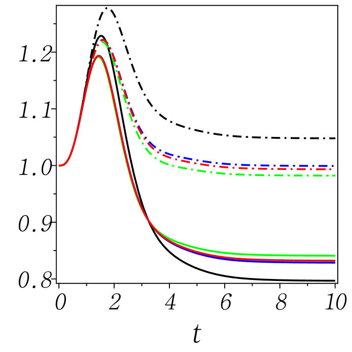
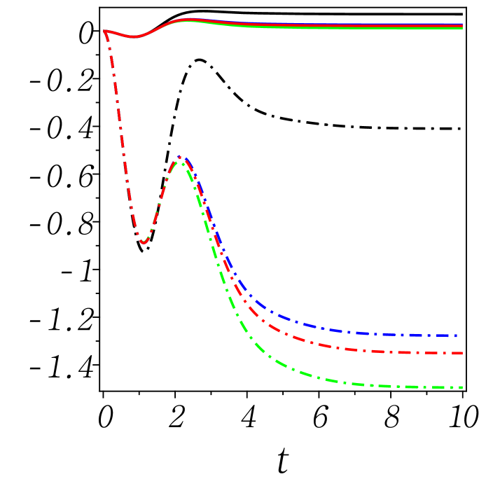
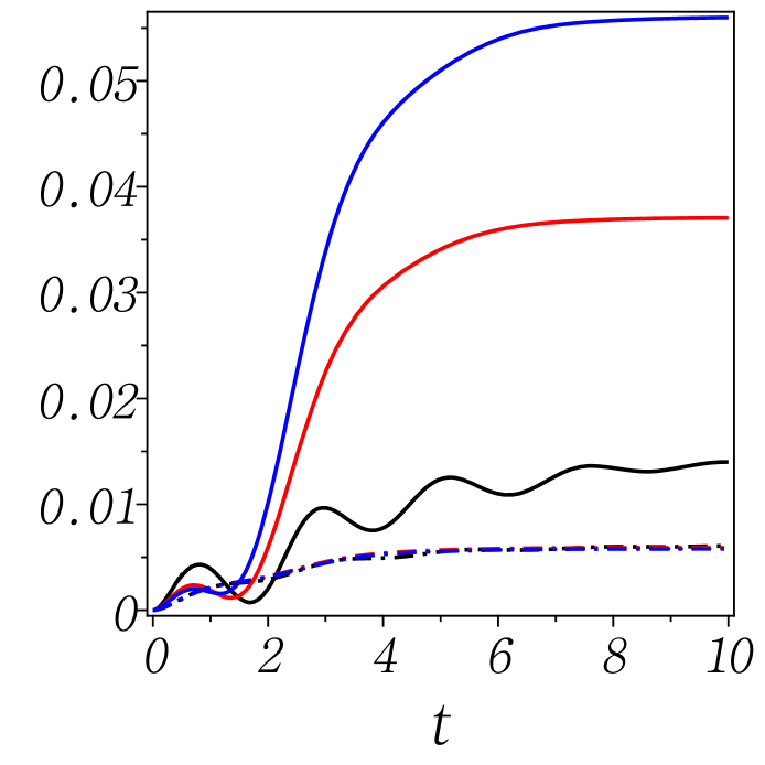
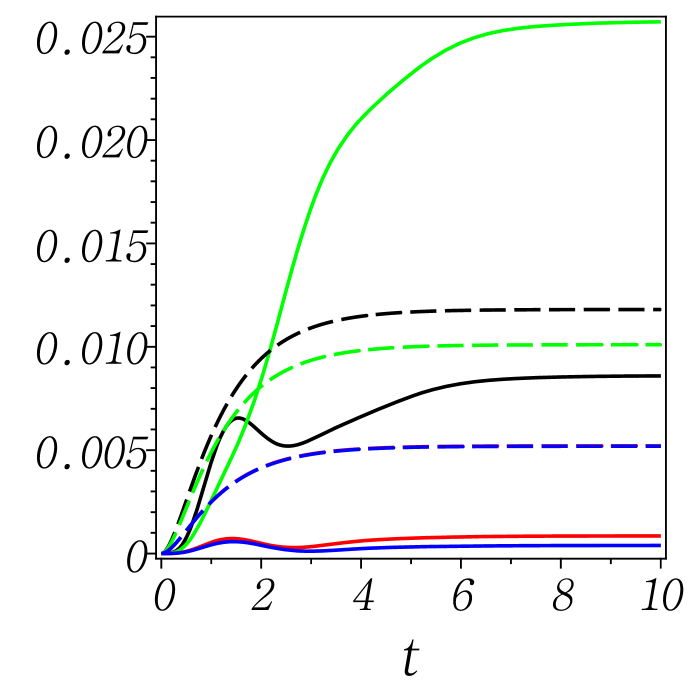
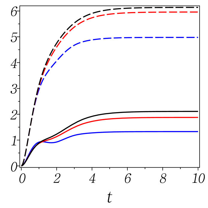
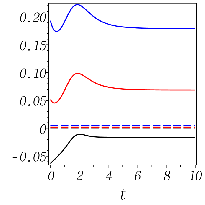
in terms of the coefficients $\tilde{a}_{1}(t),\tilde{b}_{1}(t)$ and $\tilde{c}_{1}(t)$ in (56a)-(56c). Here, the parameter $D(t)=\pm\{\tilde{a}_{1}(t)\,\tilde{c}_{1}(t)/\tilde{b}_{1}^{2}(t)-1\}^{1/2}\in{\mathbb{R}}$ or $i{\mathbb{R}}$ as given in Appendix and so $f(t)$ and $g(t)\in i{\mathbb{R}}$ in (82). As shown, the time-dependency of the reduced density operator in (59) consists entirely in $B_{1}(t)$ and $\Phi_{1}(t)$. Figs. 1-2 demonstrate their behaviors versus time for, e.g., $k(t)=k_{0}\,(2-e^{-t})$ within the Drude damping model. Applying exactly the same technique, we can also derive the reduced density operator $\langle q|\hat{{\mathcal{R}}}^{(w)}_{2}(t)|q^{\prime}\rangle$ in closed form, which is in fact identical to Eq. (59) but with replacement of $B_{1}(t),\Phi_{1}(t)\to B_{2}(t),\Phi_{2}(t)$ in terms of $\tilde{a}_{2}(t),\tilde{b}_{2}(t)$ and $\tilde{c}_{2}(t)$ for $f(t),g(t)$ and $D(t)$ therein. The normalization $\text{Tr}\,\hat{\mathcal{R}}^{(w)}_{1}(t)=\text{Tr}\,\hat{\mathcal{R}}^{(w)}_{2}(t)=1$ can easily be verified with the aid of the identity ABS74

$$\int_{-\infty}^{\infty}dx\,e^{-(ax^{2}+2bx)}\;=\;\sqrt{\frac{\pi}{a}}\,e^{\frac{b^{2}}{a}}\,.$$ (62)

It then follows that $\langle\hat{q}\rangle_{\rho_{1}(t)}\equiv\langle\hat{q}\rangle_{{\mathcal{R}}^{(w)}_{1}(t)}=0$ and $\langle\hat{p}\rangle_{\rho_{1}(t)}\equiv\langle\hat{p}\rangle_{{\mathcal{R}}^{(w)}_{1}(t)}=0$, and

$$\langle\hat{q}^{2}\rangle_{\rho_{1}(t)}\,=\,\frac{1}{B_{1}(t)}\,\langle\hat{q}^{2}\rangle_{\beta}\;\;\;;\;\;\;\langle\hat{p}^{2}\rangle_{\rho_{1}(t)}\,=\,B_{1}(t)\,\langle\hat{p}^{2}\rangle_{\beta}\,+\,\frac{4\hbar^{2}\,\Phi_{1}^{2}(t)}{B_{1}(t)}\,\frac{1}{\langle\hat{q}^{2}\rangle_{\beta}}\,.$$ (63)

From this, the instantaneous uncertainty relation also follows as

$$(\Delta q)^{2}_{\rho_{1}(t)}\,(\Delta p)^{2}_{\rho_{1}(t)}\;=\;\langle\hat{q}^{2}\rangle_{\beta}\,\langle\hat{p}^{2}\rangle_{\beta}\,+\,\frac{4\hbar^{2}\,\Phi_{1}^{2}(t)}{B_{1}^{2}(t)}\,.$$ (64)

Then the instantaneous internal energy of the coupled oscillator reads as

$${}_{1}{\mathcal{U}}_{s}(t)\,=\,\langle{}_{1}\hat{{\mathcal{H}}}_{s}(t)\rangle_{{\mathcal{R}}^{(w)}_{1}(t)}\,=\,\frac{\langle\hat{p}^{2}\rangle_{\rho_{1}(t)}}{2M}\,+\,\frac{k(t)}{2}\,\langle\hat{q}^{2}\rangle_{\rho_{1}(t)}\,.$$ (65)

Along the same line, the expectation values for the density operator $\hat{{\mathcal{R}}}^{(w)}_{2}(t)$ easily appear, respectively, as the counterparts to those in Eqs. (63) and (64) in terms of $B_{2}(t)$ and $\Phi_{2}(t)$, and so the instantaneous internal energy ${}_{2}{\mathcal{U}}_{s}(t)=\langle{}_{2}\hat{{\mathcal{H}}}_{s}(t)\rangle_{{\mathcal{R}}^{(w)}_{2}(t)}$ will immediately follow as well.

Comments deserve here. The compact form of the density operator $\hat{{\mathcal{R}}}^{(w)}_{1}(t)$ in (59), valid for an arbitrary variation of the spring constant $k(t)$, was clearly derived for the special initial condition $\hat{{\mathcal{R}}}(0)$ in (37), or equivalently, the canonical thermal equilibrium state $\hat{\rho}_{\beta}$ of the total system $\hat{H}_{0}$ with $[\hat{\rho}_{\beta},\hat{H}_{0}]=0$. This then gave rise to the significant simplification in form in the step from (3) to (3), which subsequently led, with the useful relations in (3), to Eq. (44) and finally Eq. (59). In the general case of the initial condition, on the other hand, it is mathematically not straightforward to obtain an explicit form of the density operator $\hat{{\mathcal{R}}}^{(w)}_{1}(t)$. Clearly, the time-dependent coefficients $\{\tilde{a}_{1}(t),\tilde{b}_{1}(t),\tilde{c}_{1}(t)\}$ in (56a)-(56c) are fundamental ingredients to the time-evolution operator in (55) and so the reduced density operator $\hat{{\mathcal{R}}}^{(w)}_{1}(t)$. Then, as shown in (3)-(3), the coefficients are expressed in terms of the parameter $h_{1}(t)$ representing the variation of the spring constant as well as the response functions $\chi_{rr}(t)$ and $\chi_{rp}(t)$, defined as the average values with respect to the initial condition $\hat{\rho}_{\beta}$ but temperature-independent indeed [cf. (18)] and reflecting the characteristics of the bath coupled to the oscillator in consideration.

It may also be worthwhile to point out that Zerbe and Hänggi derived a master equation for the reduced density operator $\hat{{\mathcal{R}}}_{1}(t)$, however, restricted to i) the periodic potential, $h_{1}(t)\,\hat{q}^{2}\to(m/2)\cdot\epsilon\,\cos(\Omega t+\varphi)\,\hat{q}^{2}$; ii) the Ohimic damping; iii) the initial state of the total system given by an uncoupled one $\hat{\rho}_{0}=\hat{\rho}_{s}\otimes\hat{\rho}_{b}$ HAE95 , whereas this is obviously not the case in our study. Accordingly, the initial state $\hat{\rho}_{0}$ cannot represent a thermal equilibrium of the coupled total system (oscillator plus bath), which is necessary for the discussion of the Clausius inequality in Sect. 5. Further, in a damping model without cut-off frequency (such as the Ohmic), which is not physically realistic, the validity of the second law in the quantum Brownian oscillator may not be guaranteed KIM07 ; KIM06 .

4 Quasi-static process and its reduced density operator of the coupled oscillator

For comparison with the above non-equilibrium processes, we discuss the corresponding quasi-static processes. Here the system of interest undergoes change infinitely slowly and so remains in equilibrium exactly in form of Eq. (37) in every single step such that for any spring constant $k$,

$$\langle q|\hat{R}_{\text{\scriptsize eq}}(k)|q^{\prime}\rangle\,=\,\frac{1}{\sqrt{2\pi\langle\hat{q}^{2}\rangle_{\beta}(k)}}\,\exp\left\{-\frac{(q+q^{\prime})^{2}}{8\,\langle\hat{q}^{2}\rangle_{\beta}(k)}-\frac{\langle\hat{p}^{2}\rangle_{\beta}(k)\cdot(q-q^{\prime})^{2}}{2\hbar^{2}}\right\}\,,$$ (66)

(valid for an arbitrary system-bath coupling strength indeed), where the initial values $\langle\hat{q}^{2}\rangle_{\beta}(k_{0})=\langle\hat{q}^{2}\rangle_{\beta}$ and $\langle\hat{p}^{2}\rangle_{\beta}(k_{0})=\langle\hat{p}^{2}\rangle_{\beta}$. Apparently, this density matrix looks different from $\langle q|\hat{{\mathcal{R}}}^{(w)}_{1}(t)|q^{\prime}\rangle$ in (59), and in general not in form of a canonical thermal state $\propto e^{-\beta\,{}_{1}\hat{{\mathcal{H}}}_{s}(t)}$ KIM10 . Eq. (59), however, reduces to its quasi-static counterpart in (66) indeed if $\dot{k}(t)\to 0$ at every single moment: As demonstrated in Fig. 2 for the parameter $\Phi_{1}(t)$ of (59), where $k(t)=k_{0}\,(2-e^{-t})$ and so $\dot{k}(\infty)\to 0$, we have $\dot{\Phi}_{1}(\infty)\to 0$. From this and the initial value $\Phi_{1}(0)=0$, it must follow that if $\dot{k}(t)$ remains infinitesimally small at every single moment, then $\Phi_{1}(t)\to 0$ always. This immediately leads to $\langle\hat{p}^{2}\rangle_{\rho_{1}(t)}\to B_{1}(t)\,\langle\hat{p}^{2}\rangle_{\beta}$ in (63), and then $\langle\hat{q}^{2}\rangle_{\rho_{1}(t)}=\langle\hat{q}^{2}\rangle_{\beta}/B_{1}(t)\to\langle\hat{q}^{2}\rangle_{\beta}(k)$ as well as $\langle\hat{p}^{2}\rangle_{\rho_{1}(t)}\to\langle\hat{p}^{2}\rangle_{\beta}(k)$ in (59). As a result, we can arrive at Eq. (66).

Consequently, without any harm we can straightforwardly adopt here, with $k_{0}\to k$, all results for the initial equilibrium state $\hat{R}_{\text{\scriptsize eq}}(k_{0})=\hat{{\mathcal{R}}}(0)$ obtained in KIM10 ; we can introduce an uncoupled effective oscillator

$$\hat{H}_{\text{\scriptsize eff}}^{\star}(k_{0})\;=\;\frac{\hat{p}^{2}}{2\,M_{\text{\scriptsize eff}}^{\star}(k_{0})}\,+\,\frac{k_{\text{\scriptsize eff}}^{\star}(k_{0})}{2}\,\hat{q}^{2}$$ (67)

in the same state $\hat{R}_{\text{\scriptsize eq}}(k_{0})$, with its internal energy $U_{\text{\scriptsize eff}}^{\star}(k_{0}):=\langle\hat{H}_{\text{\scriptsize eff}}^{\star}(k_{0})\rangle_{{R}_{\text{\scriptsize eq}}(k_{0})}$, being identical to the internal energy $U_{s}(k_{0}):=\langle\hat{H}_{s}\rangle_{{R}_{\text{\scriptsize eq}}(k_{0})}$ of the coupled oscillator $\hat{H}_{s}$, as well as its von-Neumann entropy $S_{\text{\scriptsize eff}}^{\star}(k_{0})=-k_{B}\,\mbox{Tr}\{\hat{R}_{\text{\scriptsize eq}}(k_{0})\,\ln\hat{R}_{\text{\scriptsize eq}}(k_{0})\}=k_{B}\{v(k_{0})+1/2\}\,\ln\{v(k_{0})+1/2\}-k_{B}\{v(k_{0})-1/2\}\,\ln\{v(k_{0})-1/2\}$ in terms of $v(k_{0})=\sqrt{\langle\hat{q}^{2}\rangle_{\beta}(k_{0})\cdot\langle\hat{p}^{2}\rangle_{\beta}(k_{0})}/\hbar$, being identical to that of the coupled oscillator. Here the mass of the effective oscillator is given by $M_{\text{\scriptsize eff}}^{\star}(k_{0})=\langle\hat{p}^{2}\rangle_{\beta}(k_{0})/U_{s}(k_{0})$, and the effective spring constant $k_{\text{\scriptsize eff}}^{\star}(k_{0})=(k_{0}+\langle\hat{p}^{2}\rangle_{\beta}(k_{0})/\{M\,\langle\hat{q}^{2}\rangle_{\beta}(k_{0})\})/2$. Subsequently the effective frequency easily follows as

$$\omega_{\text{\scriptsize eff}}^{\star}(k_{0})\,=\,\frac{1}{2M}\sqrt{\frac{\langle\hat{p}^{2}\rangle_{\beta}(k_{0})}{\langle\hat{q}^{2}\rangle_{\beta}(k_{0})}}\,+\,\frac{k_{0}}{2}\sqrt{\frac{\langle\hat{q}^{2}\rangle_{\beta}(k_{0})}{\langle\hat{p}^{2}\rangle_{\beta}(k_{0})}}\,,$$ (68)

which also allows us to have

$$U_{\text{\scriptsize eff}}^{\star}(k_{0})\;=\;\omega_{\text{\scriptsize eff}}^{\star}(k_{0})\,\sqrt{\langle\hat{q}^{2}\rangle_{\beta}(k_{0})\cdot\langle\hat{p}^{2}\rangle_{\beta}(k_{0})}\,.$$ (69)

Therefore, for the single state $\hat{R}_{\text{\scriptsize eq}}(k_{0})$ we now have two different pictures of the Hamiltonian in consideration, namely, the coupled oscillator $\hat{H}_{s}(k_{0})$ and its uncoupled effective counterpart $\hat{H}_{\text{\scriptsize eff}}^{\star}(k_{0})$.

Then it can be shown that the effective picture $\hat{H}_{\text{\scriptsize eff}}^{\star}(k_{0})$ is, remarkably enough, exactly in the canonical thermal equilibrium state $\hat{R}_{\text{\scriptsize eq}}(k_{0})\propto\exp\{-\beta_{\text{\scriptsize eff}}^{\star}(k_{0})\cdot\hat{H}_{\text{\scriptsize eff}}^{\star}(k_{0})\}$, where $\beta_{\text{\scriptsize eff}}^{\star}(k_{0})=1/\{k_{B}\,T_{\text{\scriptsize eff}}^{\star}(k_{0})\}$ with the well-defined effective temperature $T_{\text{\scriptsize eff}}^{\star}(k_{0})=\hbar\omega_{\text{\scriptsize eff}}^{\star}(k_{0})/(k_{B}\,\ln\{1/\xi_{\beta}(k_{0})\})$. Here $\xi_{\beta}(k_{0})=\{v(k_{0})-1/2\}/\{v(k_{0})+1/2\}$. From this, it also follows that

$$\langle\hat{q}^{2}\rangle_{\beta}(k_{0}) = \frac{\hbar}{2M_{\text{\scriptsize eff}}^{\star}(k_{0})\cdot\omega_{\text{\scriptsize eff}}^{\star}(k_{0})}\;\coth\left\{\frac{\beta_{\text{\scriptsize eff}}^{\star}(k_{0})\cdot\hbar\,\omega_{\text{\scriptsize eff}}^{\star}(k_{0})}{2}\right\}$$ (70a)

$$\langle\hat{p}^{2}\rangle_{\beta}(k_{0}) = \frac{M_{\text{\scriptsize eff}}^{\star}(k_{0})\cdot\hbar\,\omega_{\text{\scriptsize eff}}^{\star}(k_{0})}{2}\;\coth\left\{\frac{\beta_{\text{\scriptsize eff}}^{\star}(k_{0})\cdot\hbar\,\omega_{\text{\scriptsize eff}}^{\star}(k_{0})}{2}\right\}\,.$$ (70b)

As a result, for the quasi-static process (66) we can take all expressions from Eq. (67) to (70b) simply with replacement of $k_{0}\to k(t)$; e.g., the internal energy $U_{\text{\scriptsize eff}}^{\star}\{k(t)\}=U_{s}\{k(t)\}=\langle\hat{p}^{2}\rangle_{\beta}\{k(t)\}/2M+k(t)\,\langle\hat{q}^{2}\rangle_{\beta}\{k(t)\}/2$, which is surely different from its non-equilibrium counterpart ${}_{1}{\mathcal{U}}_{s}(t)$ in (65) (note that the time-dependency of the quasi-static quantities comes entirely through the $k$-value specified by time $t$). Needless to say, in case that the coupling constants $c_{j}\to 0$, then $\hat{H}_{\text{\scriptsize eff}}^{\star}(k)\to\hat{H}_{s}(k)$ as well as $T_{\text{\scriptsize eff}}^{\star}(k)\to T$. Also, for the upcoming numerical analysis it is useful to point out that in the Drude damping model we substitute $\omega_{0}^{2}\to\omega^{2}(k)=k(t)/M$ into Eq. (17), which will give the expression of the parameter $\Omega(k)$ in terms of $\{\omega(k),\omega_{d},\gamma_{o}\}$, and then those of $\gamma(k)=\omega_{d}-\Omega(k)$ and ${\bf w}_{0}^{2}(k)=\{k(t)/M\}\{\omega_{d}/\Omega(k)\}$, respectively. And $z_{1}(k)=\gamma(k)/2+i{\bf w}_{1}(k)$ and $z_{2}(k)=\gamma(k)/2-i{\bf w}_{1}(k)$, where ${\bf w}_{1}(k)=\sqrt{\{{\bf w}_{0}(k)\}^{2}-\{\gamma(k)/2\}^{2}}$.

It is also interesting to consider a temporal behavior of a distance between the non-equilibrium state $\hat{{\mathcal{R}}}^{(w)}_{1}(t)$ and its quasi-static counterpart $\hat{R}_{\text{\scriptsize eq}}\{k(t)\}$. To do so, we adopt a well-defined measure $D_{a}^{2}(t):=\text{Tr}\,(\hat{{\mathcal{R}}}^{(w)}_{1}(t)-\hat{R}_{\text{\scriptsize eq}}\{k(t)\})^{2}$ GRA98 , which is, independent of the dimension of the Liouville space, between 0 and 2. With the aid of ABS74

$$\textstyle\int_{-\infty}^{\infty}dq\,dq^{\prime}\exp\left\{-a(q+q^{\prime})^{2}-b(q-q^{\prime})^{2}+ic(q^{2}-q^{\prime 2})\right\}\,=\,\frac{\pi}{\sqrt{4ab+c^{2}}}$$ (71)

we can obtain

$$D_{a}^{2}(t)\,=\,\frac{\hbar}{2}\left(\frac{1}{\sqrt{\langle\hat{q}^{2}\rangle_{\beta}\,\langle\hat{p}^{2}\rangle_{\beta}}}+\frac{1}{\sqrt{\langle\hat{q}^{2}\rangle_{\beta}\{k(t)\}\,\cdot\langle\hat{p}^{2}\rangle_{\beta}\{k(t)\}}}\right)\,-$$ (72)

$$\frac{2\hbar\sqrt{B_{1}(t)\,\langle\hat{q}^{2}\rangle_{\beta}}}{\sqrt{\left(B_{1}(t)\,\langle\hat{q}^{2}\rangle_{\beta}\{k(t)\}+\langle\hat{q}^{2}\rangle_{\beta}\right)\left(B_{1}(t)\,\langle\hat{p}^{2}\rangle_{\beta}+\langle\hat{p}^{2}\rangle_{\beta}\{k(t)\}\right)\,\langle\hat{q}^{2}\rangle_{\beta}+4\hbar^{2}\,\Phi_{1}^{2}(t)\,\langle\hat{q}^{2}\rangle_{\beta}\{k(t)\}}}\,.$$

In Fig. 3 this measure for $k(t)=k_{0}\,(2-e^{-t})$ is demonstrated for different parameters. Similarly we can also have

$$D_{b}^{2}(t) := \mbox{Tr}\,\{\hat{{\mathcal{R}}}^{(w)}_{1}(t)-\hat{{\mathcal{R}}}(0)\}^{2}\,=\,\frac{\hbar}{\sqrt{\langle\hat{q}^{2}\rangle_{\beta}\,\langle\hat{p}^{2}\rangle_{\beta}}}-\frac{2\hbar\sqrt{B_{1}(t)}}{\sqrt{\{B_{1}(t)+1\}^{2}\,\langle\hat{q}^{2}\rangle_{\beta}\,\langle\hat{p}^{2}\rangle_{\beta}+4\hbar^{2}\,\Phi_{1}^{2}(t)}}$$

$$D_{c}^{2}(t) := \mbox{Tr}\,\{\hat{R}_{\text{\scriptsize eq}}\{k(t)\}-\hat{R}_{\text{\scriptsize eq}}(k_{0})\}^{2}\,=\,\frac{\hbar}{2}\left(\frac{1}{\sqrt{\langle\hat{q}^{2}\rangle_{\beta}\,\langle\hat{p}^{2}\rangle_{\beta}}}+\frac{1}{\sqrt{\langle\hat{q}^{2}\rangle_{\beta}\{k(t)\}\cdot\langle\hat{p}^{2}\rangle_{\beta}\{k(t)\}}}\right)$$ (73)

$$-\frac{2\hbar}{\sqrt{\left(\langle\hat{q}^{2}\rangle_{\beta}+\langle\hat{q}^{2}\rangle_{\beta}\{k(t)\}\right)\left(\langle\hat{p}^{2}\rangle_{\beta}+\langle\hat{p}^{2}\rangle_{\beta}\{k(t)\}\right)}}$$

(cf. Fig. 4). Finally it should be stated that all results in Sect. 4 also hold for the density operator $\hat{{\mathcal{R}}}^{(w)}_{2}(t)$ for the mass variation, simply by replacement of the subscripts $1\to 2$ and $k(t)\to M(t)$ of all pertinent parameters.

5 The second law of thermodynamics

Based on the results found in the previous sections, we will explicitly discuss the second law of thermodynamics in the quantum Brownian oscillator. To address this issue, we need first of all the first law of thermodynamics

$$dU_{s}\,=\,\sum_{n}\textstyle\left(E_{n}\,dp_{n}\,+\,p_{n}\,dE_{n}\right)\,,$$ (74)

where $\sum p_{n}dE_{n}=\mbox{Tr}(\hat{\rho}\,d\hat{{\mathcal{H}}}_{s})=\delta{\mathcal{W}}_{s}$ corresponds to an amount of work on the coupled oscillator, and $\sum E_{n}dp_{n}=\mbox{Tr}(\hat{{\mathcal{H}}}_{s}\,d\hat{\rho})=\delta{\mathcal{Q}}_{s}$ an amount of heat added to the oscillator ALL00 . Next we consider a specific non-equilibrium process (I), leading to a finite (and so experimentally measurable), rather than infinitesimal, change in those thermodynamic quantities, in which the system begins and ends in thermal equilibrium states but is driven away from thermal equilibrium at intermediate times. Then an amount of the work along the process starting with the initial state (37) is given, with no harm, by

$${}_{1}{\mathcal{W}}_{s}(t)\,=\,\int_{0}^{t}d\tau\,\dot{k}\,\left\langle\frac{\partial{}_{1}\hat{{\mathcal{H}}}_{s}(\tau)}{\partial k}\right\rangle_{{\mathcal{R}}^{(w)}_{1}(\tau)}\,=\,\frac{1}{2}\int_{0}^{t}d\tau\,\dot{k}\,\langle\hat{q}^{2}\rangle_{\rho_{1}(\tau)}$$ (75)

[cf. Eq. (63)]. Note here that at the end point $\tau=t$, the system ${}_{1}\hat{{\mathcal{H}}}_{s}(t)$ may not necessarily be in an equilibrium state but relax to the end equilibrium state $\hat{R}_{\text{\scriptsize eq}}\{k(t)\}$ in (66). However, no work is performed during this final stage of thermal relaxation. Then the second law in its Kelvin-Planck form CAL85 that this work cannot be less than its quasi-static counterpart is expressed as

$${}_{1}{\mathcal{W}}_{s}(t)\,\geq\,W_{s}\{k(t)\}\,,$$ (76)

where the work along the quasi-static process

$$W_{s}\{k(t)\}\,=\,\int_{0}^{t}d\tau\,\dot{k}\,\left\langle\frac{\partial{}_{1}\hat{{\mathcal{H}}}_{s}(\tau)}{\partial k}\right\rangle_{R_{{\text{\scriptsize eq}}}\{k(\tau)\}}\,=\,\frac{1}{2}\int_{0}^{t}d\tau\,\dot{k}\,\langle\hat{q}^{2}\rangle_{\beta}\{k(\tau)\}\,,$$ (77)

Fig. 5 demonstrates the validity of this inequality and so that of the second law. Notably, however, based on the fact that the equilibrium density operator $\hat{R}_{\text{\scriptsize eq}}\{k(\tau)\}$ is in general not in form of a canonical thermal state for the coupled oscillator ${}_{1}\hat{{\mathcal{H}}}_{s}(\tau)$ in consideration (rather than its uncoupled counterpart $\hat{H}_{\text{\scriptsize eff}}^{\star}\{k(\tau)\}$), it can easily be shown that the quasi-static work $W_{s}\{k(t)\}$ cannot be interpreted as a well-defined free energy change of the coupled oscillator ${}_{1}\hat{{\mathcal{H}}}_{s}(\tau)$ where $0\leq\tau\leq t$.

Here it is also worthwhile to shortly point out that there is an alternative formulation based on the partition function ${\mathcal{Z}}_{1}\{k(\tau)\}=\mbox{Tr}\,e^{-\beta\,\hat{{\mathcal{H}}}_{1}(\tau)}/\mbox{Tr}_{b}\,e^{-\beta\hat{H}_{b}}$, where $\beta=1/(k_{B}\,T)$ and the total Hamiltonian $\hat{{\mathcal{H}}}_{1}(\tau)={}_{1}\hat{{\mathcal{H}}}_{s}(\tau)+\hat{H}_{b}+\hat{H}_{sb}$ HAE05 ; KIM07 ; FOR06 ; KIM06 ; FOR85 ; HOE05 ; GEL09 ; HIL11 . This immediately leads to the well-defined free energy ${\mathcal{F}}_{1}\{k(\tau)\}=-\ln{\mathcal{Z}}_{1}\{k(\tau)\}/\beta$. As discussed in detail in KIM10 (the last paragraph of Sect. 3 thereof), however, the free energy ${\mathcal{F}}_{1}\{k(\tau)\}$, containing by definition the coupling-induced ($\hat{H}_{sb}$) contribution, is not valid for the coupled oscillator ${}_{1}\hat{{\mathcal{H}}}_{s}(\tau)$ alone.

Next we discuss the second law in terms of heat. To do so, we first take into account the internal energy $U_{s}\{k(\tau)\}\stackrel{{\scriptstyle!}}{{=}}U_{\text{\scriptsize eff}}^{\star}\{k(\tau)\}$ of the coupled oscillator ${}_{1}\hat{{\mathcal{H}}}_{s}(\tau)$ as well as its uncoupled counterpart $\hat{H}_{\text{\scriptsize eff}}^{\star}\{k(\tau)\}$. The first law of thermodynamics then tells us that the internal energy change along the quasi-static process is $U_{s}\{k(\tau)\}|^{t}_{0}=Q_{s}\{k(t)\}+W_{s}\{k(t)\}\stackrel{{\scriptstyle!}}{{=}}Q_{\text{\scriptsize eff}}^{\star}\{k(t)\}+W_{\text{\scriptsize eff}}^{\star}\{k(t)\}$, which is tantamount to ${}_{1}{\mathcal{Q}}_{\text{\scriptsize eff}}(t)+{}_{1}{\mathcal{W}}_{\text{\scriptsize eff}}(t)$ along the corresponding non-equilibrium process (I) above. Here the non-equilibrium effective work ${}_{1}{\mathcal{W}}_{\text{\scriptsize eff}}(t)$ and its quasi-static counterpart $W_{\text{\scriptsize eff}}^{\star}\{k(t)\}$ can be obtained directly from Eqs. (75) and (77), respectively, with replacement of the coupled oscillator ${}_{1}\hat{{\mathcal{H}}}_{s}(\tau)$ by its counterpart $\hat{H}_{\text{\scriptsize eff}}^{\star}\{k(\tau)\}$ such that

$${}_{1}{\mathcal{W}}_{\text{\scriptsize eff}}(t) = \frac{1}{2}\int_{0}^{t}d\tau\,\dot{k}(\tau)\,\left(\langle\hat{p}^{2}\rangle_{\rho_{1}(\tau)}\,\partial_{k}\frac{1}{M_{\text{\scriptsize eff}}^{\star}\{k(\tau)\}}+\langle\hat{q}^{2}\rangle_{\rho_{1}(\tau)}\,\partial_{k}\,k_{\text{\scriptsize eff}}^{\star}\{k(\tau)\}\right)$$ (78)

$$W_{\text{\scriptsize eff}}^{\star}\{k(t)\} = \frac{1}{2}\int_{0}^{t}d\tau\,\dot{k}(\tau)\,\left(\langle\hat{p}^{2}\rangle_{\beta}\{k(\tau)\}\cdot\partial_{k}\frac{1}{M_{\text{\scriptsize eff}}^{\star}\{k(\tau)\}}+\langle\hat{q}^{2}\rangle_{\beta}\{k(\tau)\}\cdot\partial_{k}\,k_{\text{\scriptsize eff}}^{\star}\{k(\tau)\}\right)$$

where

$$\partial_{k}\frac{1}{M_{\text{\scriptsize eff}}^{\star}(k)} = \frac{\langle\hat{q}^{2}\rangle_{\beta}(k)}{2\,\langle\hat{p}^{2}\rangle_{\beta}(k)}+\frac{k(t)}{2}\left\{\frac{\partial_{k}\langle\hat{q}^{2}\rangle_{\beta}(k)}{\langle\hat{p}^{2}\rangle_{\beta}(k)}-\frac{\langle\hat{q}^{2}\rangle_{\beta}(k)\cdot\partial_{k}\langle\hat{p}^{2}\rangle_{\beta}(k)}{\langle\hat{p}^{2}\rangle_{\beta}^{2}(k)}\right\}$$

$$\partial_{k}\,k_{\text{\scriptsize eff}}^{\star}(k) = \frac{1}{2}\left(1+\frac{1}{M}\left\{\frac{\partial_{k}\langle\hat{p}^{2}\rangle_{\beta}(k)}{\langle\hat{q}^{2}\rangle_{\beta}(k)}-\frac{\langle\hat{p}^{2}\rangle_{\beta}(k)\cdot\partial_{k}\langle\hat{q}^{2}\rangle_{\beta}(k)}{\langle\hat{q}^{2}\rangle_{\beta}^{2}(k)}\right\}\right)$$ (79b)

[note the discussion just before Eq. (68) with replacement of $k_{0}\to k$]. And the quasi-static effective heat $Q_{\text{\scriptsize eff}}^{\star}\{k(t)\}$ can be expressed as $\int_{0}^{t}d\tau\,\dot{k}(\tau)\,T_{\text{\scriptsize eff}}^{\star}\{k(\tau)\}\cdot\partial_{k}S_{N}\{k(\tau)\}$ in terms of the well-defined effective equilibrium temperature. Here the von-Neumann entropy $S_{N}(k)$ is identified with the thermal entropy of the effective oscillator as

$$\frac{\partial}{\partial k}Q_{\text{\scriptsize eff}}^{\star}(k) = \frac{1}{2M_{\text{\scriptsize eff}}^{\star}(k)}\,\frac{\partial}{\partial k}\langle\hat{p}^{2}\rangle_{\beta}(k)\,+\,\frac{k_{\text{\scriptsize eff}}^{\star}(k)}{2}\,\frac{\partial}{\partial k}\langle\hat{q}^{2}\rangle_{\beta}(k)$$

$$= \frac{\hbar\omega_{\text{\scriptsize eff}}^{\star}(k)}{4}\left\{\frac{\partial}{\partial k}\ln\xi_{\beta}(k)\right\}\left\{\text{csch}\frac{\ln\xi_{\beta}(k)}{2}\right\}^{2}\,=\,T_{\text{\scriptsize eff}}^{\star}(k)\,\frac{\partial}{\partial k}S_{N}(k)$$

[cf. Eqs. (70a) and (70b)].

Now let ${}_{1}{\mathcal{W}}_{\text{\scriptsize s-eff}}(t):={}_{1}{\mathcal{W}}_{s}(t)-{}_{1}{\mathcal{W}}_{\text{\scriptsize eff}}(t)$, which can be interpreted as the work needed for “switch of picture” from the uncoupled effective oscillator to its coupled counterpart along the non-equilibrium process (I), and its quasi-static counterpart $W_{\text{\scriptsize s-eff}}\{k(t)\}:=W_{s}\{k(t)\}-W_{\text{\scriptsize eff}}^{\star}\{k(t)\}$. Substituting these two work functions into Inequality (76) and applying the above first law, we can immediately derive a generalized Clausius inequality

$${}_{1}{\mathcal{Q}}_{\text{\scriptsize eff}}(t)\,\leq\,Q_{\text{\scriptsize eff}}^{\star}\{k(t)\}\,+\,{}_{1}\Delta_{\text{\scriptsize s-eff}}(t)\,,$$ (81)

where ${}_{1}\Delta_{\text{\scriptsize s-eff}}(t):={}_{1}{\mathcal{W}}_{\text{\scriptsize s-eff}}(t)-W_{\text{\scriptsize s-eff}}\{k(t)\}$ with ${}_{1}\Delta_{\text{\scriptsize s-eff}}(0)=0$. Therefore, in the picture of effective oscillator we hold the standard form of the Clausius inequality in terms of the well-defined (effective) temperature, but with the additional term ${}_{1}\Delta_{\text{\scriptsize s-eff}}(t)$. This inequality can be considered as a consistent generalization of the Clausius equality $\delta{}_{1}{\mathcal{Q}}_{\text{\scriptsize eff}}=T_{\text{\scriptsize eff}}^{\star}\,\partial_{k}S_{N}$ valid for the quasi-static process, introduced in KIM10 . Obviously, the extra term ${}_{1}\Delta_{\text{\scriptsize s-eff}}(t)$ identically vanishes in this case. And in the vanishing coupling limit ($c_{j}\to 0$), where $T_{\text{\scriptsize eff}}^{\star}(k)\to T$ as well as both ${}_{1}{\mathcal{W}}_{\text{\scriptsize s-eff}}(t)\to 0$ and $W_{\text{\scriptsize s-eff}}\{k(t)\}\to 0$ leading to ${}_{1}\Delta_{\text{\scriptsize s-eff}}(t)\to 0$, we can easily recover the ordinary form of the Clausius inequality in terms of the equilibrium temperature of the total system. In fact, in the high-temperature limit, where the thermal fluctuation in the coupled oscillator is predominant to the system-bath coupling $\hat{H}_{sb}$, the ordinary Clausius inequality follows as expected. In the low-temperature limit, on the other hand, the additional term ${}_{1}\Delta_{\text{\scriptsize s-eff}}(t)$ may not be neglected COM11 ; in Fig. 6 we compare the incomplete Clausius inequality ${}_{1}{\mathcal{Q}}_{\text{\scriptsize eff}}(t)\leq Q_{\text{\scriptsize eff}}^{\star}\{k(t)\}$ (with no violation) with its complete counterpart in (81). As a result, we see that Inequality (81) is a generalized Clausius inequality representing the second law in the quantum Brownian oscillator, without any violation. Finally it should again be stated that all results in Sect. 5 also hold for the density operator $\hat{{\mathcal{R}}}^{(w)}_{2}(t)$, simply by replacement of the subscripts $1\to 2$ and $k(t)\to M(t)$ of all pertinent parameters.

6 Conclusion

In summary, we have analytically studied non-equilibrium dynamics in the quantum Brownian oscillator and then systematically discussed the second law of thermodynamics. We have first derived a closed expression for the time-dependent reduced density operator of the coupled oscillator in the weak-coupling limit along the non-equilibrium process. Based on this density operator, we have found a generalized Clausius inequality in terms of the “effective” parameters, which indisputably reveals the robustness of the second law in the quantum regime. In introducing the effective picture, we reasonably required all thermodynamic variables to exist and to obey the basic relationships, especially the first and the second laws. This method, as given, works for the harmonic oscillator but cannot easily generalized to apply to a broader class of quantum systems. Therefore the question about the (rigorous) validity of the second law for such systems remains open.

Our finding can be considered as a consistent generalization of the Clausius equality valid for the quasi-static process, introduced in KIM10 . We believe that this inequality will provide a useful starting point for later useful discussions of quantum thermodynamics and quantum information theory within the quantum Browian oscillator as a prototype of quantum dissipative systems; as an example, a consistent quantum generalization of the Landauer principle representing the computational irreversibility may be in immediate consideration, which can be understood as a simple logical consequence of the Clausius inequality LAN61 ; BEN03 . Lastly, it is also desirable to numerically study the non-equilibrium dynamics in this system in the genuine strong-coupling limit as the next task.

Appendix A : Derivation of the density matrix in Eq. (59)

From comparison of Eqs. (55) and (57), it easily follows that $\hat{M}\to y\partial_{y}+\partial_{z}z$ and $\hat{A}\to yz$ and $\hat{B}\to\partial_{y}\partial_{z}$, and so $\alpha\to 2$ and $m\to-1$ and $r\to 0$. Let $\lambda\to\tilde{b}_{1}(t)$ and $\mu\to\tilde{a}_{1}(t)/i\hbar\,\tilde{b}_{1}(t)$ and $\nu\to i\hbar\,\tilde{c}_{1}(t)/\tilde{b}_{1}(t)$. Then we have $d\to 0$ and $D^{2}\to\tilde{a}_{1}(t)\,\tilde{c}_{1}(t)/\tilde{b}_{1}^{2}(t)-1$ and

$$\displaystyle f\to\frac{1}{i\hbar}\,\frac{\tilde{a}_{1}(t)}{\tilde{b}_{1}(t)}\,\frac{\tan\{\tilde{b}_{1}(t)\,D\}}{D-\tan\{\tilde{b}_{1}(t)\,D\}}\;\;\;;\;\;\;g\to i\hbar\,\frac{\tilde{c}_{1}(t)}{\tilde{b}_{1}(t)}\,\frac{\tan\{\tilde{b}_{1}(t)\,D\}}{D-\tan\{\tilde{b}_{1}(t)\,D\}}$$ (82)

$$\displaystyle\kappa\to\ln\left|\frac{D}{D\cos\{\tilde{b}_{1}(t)\,D\}-\sin\{\tilde{b}_{1}(t)\,D\}}\right|\,.$$ (83)

With the aid of (57) and (58), Eq. (55) can then be rewritten as

$$T\,\exp\left\{-\frac{i}{\hbar}\,\hat{J}_{1}(t)\right\}\,=\,\exp\left(\kappa\,y\partial_{y}\right)\,\exp\left(\kappa\,\partial_{z}z\right)\,\exp\left(f\,e^{-2\kappa}yz\right)\,\exp\left(g\,\partial_{y}\partial_{z}\right)\,.$$ (84)

Substituting (84) into (44) and then using the identity $e^{c\,x\partial_{x}}F(x)=F(e^{c}\,x)$ for a function $F$ DON07 and $\partial_{z}z=1+z\partial_{z}$, we can easily obtain

$$\langle q|\hat{{\mathcal{R}}}^{(w)}_{1}(t)|q^{\prime}\rangle\,=\,\left(e^{\kappa}\,e^{fyz}\right)\cdot\left\{e^{g\partial_{y}\partial_{z}}\,\langle q|\hat{{\mathcal{R}}}(0)|q^{\prime}\rangle\right\}^{y\to e^{\kappa}y}_{z\to e^{\kappa}z}$$ (85)

where the initial equilibrium density operator in (37) is then expressed in terms of $y$ and $z$ as

$$\langle q|\hat{{\mathcal{R}}}(0)|q^{\prime}\rangle\,=\,\frac{1}{\sqrt{2\pi\,\langle\hat{q}^{2}\rangle_{\beta}}}\,\exp\left(-\frac{1}{8\,\langle\hat{q}^{2}\rangle_{\beta}}y^{2}-\frac{\langle\hat{p}^{2}\rangle_{\beta}}{2\hbar^{2}}z^{2}\right)\,.$$ (86)

Let $e^{g\partial_{y}\partial_{z}}\,\langle q|\hat{{\mathcal{R}}}(0)|q^{\prime}\rangle=e^{u\partial_{\tilde{y}}\partial_{\tilde{z}}}\,\exp\left(-\tilde{y}^{2}-\tilde{z}^{2}\right)=:G(\tilde{y},\tilde{z})$ in Eq. (85) with the aid of (86), where $\tilde{y}:=y/\sqrt{8\,\langle\hat{q}^{2}\rangle_{\beta}}$ and $\tilde{z}:=z\sqrt{\langle\hat{p}^{2}\rangle_{\beta}/2\hbar^{2}}$, and $u:=(g/4\hbar)\sqrt{\langle\hat{p}^{2}\rangle_{\beta}/\langle\hat{q}^{2}\rangle_{\beta}}$. We subsequently consider the expansion

$$G(\tilde{y},\tilde{z}) = \sum_{n=0}^{\infty}\frac{1}{n!}\,u^{n}\,\left(\partial_{\tilde{y}}\,\partial_{\tilde{z}}\right)^{n}\,\exp\left(-\tilde{y}^{2}-\tilde{z}^{2}\right)$$ (87)

$$= \sum_{n=0}^{\infty}\frac{1}{n!}\,u^{n}\,H_{n}(\tilde{y})\,H_{n}(\tilde{z})\,\exp\left(-\tilde{y}^{2}-\tilde{z}^{2}\right)\,.$$ (88)

Here we used an identity of the Hermite polynomial, $H_{n}(x)=(-1)^{n}\,e^{x^{2}}(d/dx)^{n}\,e^{-x^{2}}$ ABS74 . The Mehler formula MEH38 ; SZE39

$$\sum_{n=0}^{\infty}\frac{1}{n!}\,u^{n}\,H_{n}(x_{1})\,H_{n}(x_{2})\;=\;\frac{1}{\sqrt{1-4u^{2}}}\,\exp\left\{\frac{4u\,x_{1}x_{2}-4\left(x_{1}^{2}+x_{2}^{2}\right)u^{2}}{1-4u^{2}}\right\}$$ (89)

then allows us to have

$$G(\tilde{y},\tilde{z})\;=\;\frac{1}{\sqrt{1-4u^{2}}}\,\exp\left(\frac{4u\,\tilde{y}\tilde{z}-\tilde{y}^{2}-\tilde{z}^{2}}{1-4u^{2}}\right)\,.$$ (90)

From Eqs. (83), (85) and (90) we can finally obtain Eq. (59).

Fig. 1: (Color online) $B_{1}(t)$ versus time $t$ for spring constant $k(t)=k_{0}\,(2-e^{-t})$ and dimensionless temperature $k_{B}T/\hbar\omega_{0}$ [cf. Eq. (LABEL:eq:density_matrix21)]; dashdot: $T=10$ (high temperature), and solid: $T=0.01$ (low temperature). Here $\hbar=k_{B}=\omega_{0}=M=k_{0}=\gamma_{0}=1$, and $\omega_{d}=5$. Since this spring constant exponentially decays with time, the coefficients $\tilde{a}_{1}(t),\tilde{b}_{1}(t)$ and $\tilde{c}_{1}(t)$ in (56a)-(56c) should fast converge, and so the infinite sum over $n$ in (46) can be replaced by a finite sum with the upper bound $N$ not necessarily large enough. This can be verified here by considering $N=1,2,3$ and $4$. From top to bottom (at $t=10$), (black dashdot: $N=1$), (blue dashdot: $N=3$), (red dashdot: $N=4$), and (green dashdot: $N=2$); (green solid: $N=2$), (red solid: $N=4$), (blue solid: $N=3$), and (black solid: $N=1$). From this numerical result with an oscillating and fast converging behavior of $B_{1}(t)$ with increasing $N$, we adopt $\{B_{1}(t)|_{N=3}+B_{1}(t)|_{N=4}\}/2$ as a numerical fitting of $B_{1}(t)$, which will be used for later numerical studies.

Fig. 2: (Color online) $\Phi_{1}(t)$ versus time $t$ for spring constant $k(t)=k_{0}\,(2-e^{-t})$ and dimensionless temperature $k_{B}T/\hbar\omega_{0}$ [cf. Eq. (61)]; dashdot: $T=10$ (high temperature), and solid: $T=0.01$ (low temperature). Here $\hbar=k_{B}=\omega_{0}=M=k_{0}=\gamma_{0}=1$, and $\omega_{d}=5$. As for Fig. 1, we consider $N=1,2,3$ and $4$. From top to bottom (at $t=10$), (black solid: $N=1$), (blue solid: $N=3$), (red solid: $N=4$), and (green solid: $N=2$); (black dashdot: $N=1$), (blue dashdot: $N=3$), (red dashdot: $N=4$), and (green dashdot: $N=2$). From this numerical result with an oscillating and fast converging behavior of $\Phi_{1}(t)$ with increasing $N$, we adopt $\{\Phi_{1}(t)|_{N=3}+\Phi_{1}(t)|_{N=4}\}/2$ as a numerical fitting of $\Phi_{1}(t)$, which will be used for later numerical studies. Especially for $T=0.01$, $\Phi_{1}(t)|_{N=3}\approx\Phi_{1}(t)|_{N=4}$ already.

Fig. 3: (Color online) $D_{a}^{2}(t)$ versus time $t$ for spring constant $k(t)=k_{0}\,(2-e^{-t})$ and dimensionless temperature $k_{B}T/\hbar\omega_{0}$ [cf. Eq. (72)]; dashdot: $T=10$ (high temperature), and solid: $T=0.01$ (low temperature). Here $\hbar=k_{B}=\omega_{0}=M=k_{0}=\gamma_{0}=1$. From top to bottom (at $t=10$), (blue solid: cut-off frequency $\omega_{d}=15$), (red solid: $\omega_{d}=5$), and (black solid: $\omega_{d}=1$); (black dashdot: $\omega_{d}=1$), (red dashdot: $\omega_{d}=5$), and (blue dashdot: $\omega_{d}=15$). The three curves at $T=10$ are almost identical.

Fig. 4: (Color online) {$D_{b}^{2}(t)$, solid} and {$D_{c}^{2}(t)$, dash} versus time $t$ for spring constant $k(t)=k_{0}\,(2-e^{-t})$ and dimensionless temperature $k_{B}T/\hbar\omega_{0}$ [cf. Eq. (4)]. Here $\hbar=k_{B}=\omega_{0}=M=k_{0}=\gamma_{0}=1$. Solid: from top to bottom (at $t=10$), (green: $T=0.01$ and $\omega_{d}=15$), (black: $T=0.01$ and $\omega_{d}=5$), (red: $T=10$ and $\omega_{d}=5$), and (blue: $T=10$ and $\omega_{d}=15$). Dash: from top to bottom (at $t=10$), (black: $T=0.01$ and $\omega_{d}=5$), (green: $T=0.01$ and $\omega_{d}=15$), and (red: $T=10$ and $\omega_{d}=5$) $\approx$ (blue: $T=10$ and $\omega_{d}=15$).

Fig. 5: (Color online) ${}_{1}{\mathcal{W}}_{s}(t)-W_{s}\{k(t)\}=:y_{5}\geq 0$ versus time $t$ for spring constant $k(t)=k_{0}\,(2-e^{-t})$ and dimensionless temperature $k_{B}T/\hbar\omega_{0}$ [cf. Eq. (76)]; dash: $T=10$ (high temperature), and solid: $T=0.01$ (low temperature). Here $\hbar=k_{B}=\omega_{0}=M=k_{0}=\gamma_{0}=1$. From top to bottom (at $t=10$), (black dash: $\omega_{d}=15$), (red dash: $\omega_{d}=5$), and (blue dash: $\omega_{d}=1$) for $y_{5}/20$, and then (black solid: $\omega_{d}=15$), (red solid: $\omega_{d}=5$), and (blue solid: $\omega_{d}=1$) for $y_{5}$.

Fig. 6: (Color online) $\{{\mathcal{I}}_{\text{\scriptsize eff}}(t)-{\mathcal{J}}_{\text{\scriptsize eff}}(t)\}/{\mathcal{J}}_{\text{\scriptsize eff}}(t)=:y_{6}$ versus time $t$ for spring constant $k(t)=k_{0}\,(2-e^{-t})$ and dimensionless temperature $k_{B}T/\hbar\omega_{0}$. Here ${\mathcal{I}}_{\text{\scriptsize eff}}(t):=Q_{\text{\scriptsize eff}}^{\star}\{k(t)\}-{}_{1}{\mathcal{Q}}_{\text{\scriptsize eff}}(t)$, and ${\mathcal{J}}_{\text{\scriptsize eff}}(t):=Q_{\text{\scriptsize eff}}^{\star}\{k(t)\}-{}_{1}{\mathcal{Q}}_{\text{\scriptsize eff}}(t)+{}_{1}\Delta_{\text{\scriptsize s-eff}}(t)$ [cf. Eq. (81)], which is identical to ${}_{1}{\mathcal{W}}_{s}(t)-W_{s}\{k(t)\}$ in Fig. 5; dash: $T=10$ (high temperature), and solid: $T=0.01$ (low temperature). And $\hbar=k_{B}=\omega_{0}=M=k_{0}=\gamma_{0}=1$. Solid: from top to bottom, (blue: $\omega_{d}=15$), (red: $\omega_{d}=5$), and (black: $\omega_{d}=1$). Dash: in the same order. The three curves at $T=10$ almost vanish, as expected. At $T=0.01$, we see that ${}_{1}\Delta_{\text{\scriptsize s-eff}}(t)<0$ for $\omega_{d}=5$ and $15$, immediately leading to no violation of the incomplete inequality ${\mathcal{I}}_{\text{\scriptsize eff}}(t)\geq 0$; on the other hand, ${}_{1}\Delta_{\text{\scriptsize s-eff}}(t)>0$ for $\omega_{d}=1$. However, from the fact that $y_{6}\geq-1$ in this case, there is still no violation of ${\mathcal{I}}_{\text{\scriptsize eff}}(t)\geq 0$.

Figure 1:

Figure 2:

Figure 3:

Figure 4:

Figure 5:

Figure 6:

References

• (1) I. Kim and G. Mahler, Phys. Rev. E 81, 011101 (2010).
• (2) C. Vladislav and D.P. Sheehan, Challenges to the Second Law of Thermodynamics: Theory and Experiment (Springer, New York, 2005).
• (3) J. Gemmer, M. Michel and G. Mahler, Quantum Thermodynamics (Springer, Berlin, 2004).
• (4) H.B. Callen, Thermodynamics and an Introduction to Thermostatics, 2nd ed. (John Wiley, New York, 1985).
• (5) D.P. Sheehan, Quantum Limits to the Second Law, AIP Conf. Proc. No. 643 (AIP, Melville, NY, 2002).
• (6) An introduction of the effective temperature Teffsuperscriptsubscript𝑇effT_{\text{\scriptsize eff}}^{\star} may be at variance with the zeroth law of thermodynamics, which states CAL85 that if system A and system C are each in thermal contact with system B(ath) and in equilibrium, then A is also in equilibrium with C. Here, by bringing two systems in thermal contact, one means allowing a vanishingly small coupling, through which heat can be exchanged between the two systems. In the finite coupling, on the other hand, the effective temperature of (quantum system) A𝐴A can, by construction, differ from that of C𝐶C, therefore leading to a violation of the zeroth law. In fact, the violation of the zeroth law has recently been discussed in different contexts, e.g., RAM08 ; GAV11 .
• (7) A. Ramírez-Hernández, H. Larralde, and F. Leyvraz, Phys. Rev. Lett. 100, 120601 (2008).
• (8) B. Gaveau and L.S. Schulman, arXiv:1108.1962v1 (2011).
• (9) S. Deffner and E. Lutz, Phys. Rev. Lett. 105, 170402 (2010).
• (10) K. Husimi, Prog. Theor. Phys. 9, 381 (1951).
• (11) U. Weiss, Quantum Dissipative Systems, 3rd ed. (World Scientific, Singapore, 2008).
• (12) G.-L. Ingold, Dissipative Quantum Systems in Quantum Transport and Dissipation (Wiley-VCH, 1998), pp 213-248.
• (13) C. Jarzynski, J. Stat. Mech.: Theor. Exp. P09005 (2004).
• (14) P. Hänggi and G.-L. Ingold, Chaos 15, 026105 (2005).
• (15) I. Kim, Phys. Lett. A 374, 3828 (2010).
• (16) G.W. Ford, J.T. Lewis and R.F. O’Connell, Ann. Phys. (N.Y.) 185, 270 (1988).
• (17) H.B. Callen and T.A. Welton, Phys. Rev. 83, 34 (1951).
• (18) I. Kim and G. Mahler, Eur. Phys. J. B 60, 401 (2007).
• (19) M. Abramowitz and I. Stegun, Handbook of Mathematical Functions with Formulas, Graphs, and Mathematical Tables (Dover, New York, 1974).
• (20) G.W. Ford and R.F. O’Connell, Phys. Rev. Lett. 96, 020402 (2006).
• (21) D.J. Griffiths, Introduction to Quantum Mechanics, 2nd ed. (Pearson Prentice Hall, New Jersey, 2005).
• (22) R.M. Wilcox, J. Math. Phys. 8, 962 (1967).
• (23) S.-H. Dong, Factorization Method in Quantum Mechanics (Springer, Dordrecht, 2007).
• (24) H. Grabert, P. Schramm, and G.-L. Ingold, Phys. Rep. 168, 115 (1988).
• (25) C.S. Lam, J. Math. Phys. 39, 5543 (1998).
• (26) H. Mitter and K. Yamazaki, Lett. Math. Phys. 8, 321 (1984).
• (27) C. Zerbe and P. Hänggi, Phys. Rev. E 52, 1533 (1995).
• (28) I. Kim and G. Mahler, Eur. Phys. J. B 54, 405 (2006).
• (29) C.M. Granzow and G. Mahler, Appl. Phys. B 67, 733 (1998).
• (30) A.E. Allahverdyan and Th.M. Nieuwenhuizen, Phys. Rev. Lett. 85, 1799 (2000).
• (31) G.W. Ford, J.T. Lewis and R.F. O’Connell, Phys. Rev. Lett. 55, 2273 (1985).
• (32) C. Hörhammer and H. Büttner, J. Phys. A 38, 7325 (2005).
• (33) M.F. Gelin and M. Thoss, Phys. Rev. E 79, 051121 (2009).
• (34) S. Hilt, S. Shabbir, J. Anders, and E. Lutz, Phys. Rev. E 83, 030102(R) (2011).
• (35) In fact, in the strong-coupling limit, in which the effective temperature Teff(k)superscriptsubscript𝑇eff𝑘T_{\text{\scriptsize eff}}^{\star}(k) heavily differs from the total-system temperature T𝑇T, we can easily deduce from the discussion for Eqs. (78)-(81) that the Clausius inequality in this limit should also include a (non-negligible) extra term corresponding to Δs-eff1(t)subscriptsubscriptΔs-eff1𝑡{}_{1}\Delta_{\text{\scriptsize s-eff}}(t) in (81) derived in the weak-coupling limit.
• (36) R. Landauer, IBM J. Res. Dev. 5, 183 (1961).
• (37) C.H. Bennett, Stud. Hist. Philos. Mod. Phys. 34, 501 (2003), which is also available as arXiv:physics/0210005.
• (38) A. Erdélyi, Math. Z. 44, 201 (1938).
• (39) G. Szegö, Orthogonal Polynomials (American Mathematical Society, New York, 1939).
Fig. 1: (Color online) B1(t)subscript𝐵1𝑡B_{1}(t) versus time t𝑡t for spring constant k(t)=k0(2et)𝑘𝑡subscript𝑘02superscript𝑒𝑡k(t)=k_{0}\,(2-e^{-t}) and dimensionless temperature kBT/ω0subscript𝑘𝐵𝑇Planck-constant-over-2-pisubscript𝜔0k_{B}T/\hbar\omega_{0} [cf. Eq. (LABEL:eq:density_matrix21)]; dashdot: T=10𝑇10T=10 (high temperature), and solid: T=0.01𝑇0.01T=0.01 (low temperature). Here =kB=ω0=M=k0=γ0=1Planck-constant-over-2-pisubscript𝑘𝐵subscript𝜔0𝑀subscript𝑘0subscript𝛾01\hbar=k_{B}=\omega_{0}=M=k_{0}=\gamma_{0}=1, and ωd=5subscript𝜔𝑑5\omega_{d}=5. Since this spring constant exponentially decays with time, the coefficients a~1(t),b~1(t)subscript~𝑎1𝑡subscript~𝑏1𝑡\tilde{a}_{1}(t),\tilde{b}_{1}(t) and c~1(t)subscript~𝑐1𝑡\tilde{c}_{1}(t) in (56a)-(56c) should fast converge, and so the infinite sum over n𝑛n in (46) can be replaced by a finite sum with the upper bound N𝑁N not necessarily large enough. This can be verified here by considering N=1,2,3𝑁123N=1,2,3 and 444. From top to bottom (at t=10𝑡10t=10), (black dashdot: N=1𝑁1N=1), (blue dashdot: N=3𝑁3N=3), (red dashdot: N=4𝑁4N=4), and (green dashdot: N=2𝑁2N=2); (green solid: N=2𝑁2N=2), (red solid: N=4𝑁4N=4), (blue solid: N=3𝑁3N=3), and (black solid: N=1𝑁1N=1). From this numerical result with an oscillating and fast converging behavior of B1(t)subscript𝐵1𝑡B_{1}(t) with increasing N𝑁N, we adopt {B1(t)|N=3+B1(t)|N=4}/2evaluated-atsubscript𝐵1𝑡𝑁3evaluated-atsubscript𝐵1𝑡𝑁42\{B_{1}(t)|_{N=3}+B_{1}(t)|_{N=4}\}/2 as a numerical fitting of B1(t)subscript𝐵1𝑡B_{1}(t), which will be used for later numerical studies.
Fig. 2: (Color online) Φ1(t)subscriptΦ1𝑡\Phi_{1}(t) versus time t𝑡t for spring constant k(t)=k0(2et)𝑘𝑡subscript𝑘02superscript𝑒𝑡k(t)=k_{0}\,(2-e^{-t}) and dimensionless temperature kBT/ω0subscript𝑘𝐵𝑇Planck-constant-over-2-pisubscript𝜔0k_{B}T/\hbar\omega_{0} [cf. Eq. (61)]; dashdot: T=10𝑇10T=10 (high temperature), and solid: T=0.01𝑇0.01T=0.01 (low temperature). Here =kB=ω0=M=k0=γ0=1Planck-constant-over-2-pisubscript𝑘𝐵subscript𝜔0𝑀subscript𝑘0subscript𝛾01\hbar=k_{B}=\omega_{0}=M=k_{0}=\gamma_{0}=1, and ωd=5subscript𝜔𝑑5\omega_{d}=5. As for Fig. 1, we consider N=1,2,3𝑁123N=1,2,3 and 444. From top to bottom (at t=10𝑡10t=10), (black solid: N=1𝑁1N=1), (blue solid: N=3𝑁3N=3), (red solid: N=4𝑁4N=4), and (green solid: N=2𝑁2N=2); (black dashdot: N=1𝑁1N=1), (blue dashdot: N=3𝑁3N=3), (red dashdot: N=4𝑁4N=4), and (green dashdot: N=2𝑁2N=2). From this numerical result with an oscillating and fast converging behavior of Φ1(t)subscriptΦ1𝑡\Phi_{1}(t) with increasing N𝑁N, we adopt {Φ1(t)|N=3+Φ1(t)|N=4}/2evaluated-atsubscriptΦ1𝑡𝑁3evaluated-atsubscriptΦ1𝑡𝑁42\{\Phi_{1}(t)|_{N=3}+\Phi_{1}(t)|_{N=4}\}/2 as a numerical fitting of Φ1(t)subscriptΦ1𝑡\Phi_{1}(t), which will be used for later numerical studies. Especially for T=0.01𝑇0.01T=0.01, Φ1(t)|N=3Φ1(t)|N=4evaluated-atsubscriptΦ1𝑡𝑁3evaluated-atsubscriptΦ1𝑡𝑁4\Phi_{1}(t)|_{N=3}\approx\Phi_{1}(t)|_{N=4} already.
Fig. 3: (Color online) Da2(t)superscriptsubscript𝐷𝑎2𝑡D_{a}^{2}(t) versus time t𝑡t for spring constant k(t)=k0(2et)𝑘𝑡subscript𝑘02superscript𝑒𝑡k(t)=k_{0}\,(2-e^{-t}) and dimensionless temperature kBT/ω0subscript𝑘𝐵𝑇Planck-constant-over-2-pisubscript𝜔0k_{B}T/\hbar\omega_{0} [cf. Eq. (72)]; dashdot: T=10𝑇10T=10 (high temperature), and solid: T=0.01𝑇0.01T=0.01 (low temperature). Here =kB=ω0=M=k0=γ0=1Planck-constant-over-2-pisubscript𝑘𝐵subscript𝜔0𝑀subscript𝑘0subscript𝛾01\hbar=k_{B}=\omega_{0}=M=k_{0}=\gamma_{0}=1. From top to bottom (at t=10𝑡10t=10), (blue solid: cut-off frequency ωd=15subscript𝜔𝑑15\omega_{d}=15), (red solid: ωd=5subscript𝜔𝑑5\omega_{d}=5), and (black solid: ωd=1subscript𝜔𝑑1\omega_{d}=1); (black dashdot: ωd=1subscript𝜔𝑑1\omega_{d}=1), (red dashdot: ωd=5subscript𝜔𝑑5\omega_{d}=5), and (blue dashdot: ωd=15subscript𝜔𝑑15\omega_{d}=15). The three curves at T=10𝑇10T=10 are almost identical.
Fig. 4: (Color online) {Db2(t)superscriptsubscript𝐷𝑏2𝑡D_{b}^{2}(t), solid} and {Dc2(t)superscriptsubscript𝐷𝑐2𝑡D_{c}^{2}(t), dash} versus time t𝑡t for spring constant k(t)=k0(2et)𝑘𝑡subscript𝑘02superscript𝑒𝑡k(t)=k_{0}\,(2-e^{-t}) and dimensionless temperature kBT/ω0subscript𝑘𝐵𝑇Planck-constant-over-2-pisubscript𝜔0k_{B}T/\hbar\omega_{0} [cf. Eq. (4)]. Here =kB=ω0=M=k0=γ0=1Planck-constant-over-2-pisubscript𝑘𝐵subscript𝜔0𝑀subscript𝑘0subscript𝛾01\hbar=k_{B}=\omega_{0}=M=k_{0}=\gamma_{0}=1. Solid: from top to bottom (at t=10𝑡10t=10), (green: T=0.01𝑇0.01T=0.01 and ωd=15subscript𝜔𝑑15\omega_{d}=15), (black: T=0.01𝑇0.01T=0.01 and ωd=5subscript𝜔𝑑5\omega_{d}=5), (red: T=10𝑇10T=10 and ωd=5subscript𝜔𝑑5\omega_{d}=5), and (blue: T=10𝑇10T=10 and ωd=15subscript𝜔𝑑15\omega_{d}=15). Dash: from top to bottom (at t=10𝑡10t=10), (black: T=0.01𝑇0.01T=0.01 and ωd=5subscript𝜔𝑑5\omega_{d}=5), (green: T=0.01𝑇0.01T=0.01 and ωd=15subscript𝜔𝑑15\omega_{d}=15), and (red: T=10𝑇10T=10 and ωd=5subscript𝜔𝑑5\omega_{d}=5) \approx (blue: T=10𝑇10T=10 and ωd=15subscript𝜔𝑑15\omega_{d}=15).
Fig. 5: (Color online) 𝒲s1(t)Ws{k(t)}=:y50{}_{1}{\mathcal{W}}_{s}(t)-W_{s}\{k(t)\}=:y_{5}\geq 0 versus time t𝑡t for spring constant k(t)=k0(2et)𝑘𝑡subscript𝑘02superscript𝑒𝑡k(t)=k_{0}\,(2-e^{-t}) and dimensionless temperature kBT/ω0subscript𝑘𝐵𝑇Planck-constant-over-2-pisubscript𝜔0k_{B}T/\hbar\omega_{0} [cf. Eq. (76)]; dash: T=10𝑇10T=10 (high temperature), and solid: T=0.01𝑇0.01T=0.01 (low temperature). Here =kB=ω0=M=k0=γ0=1Planck-constant-over-2-pisubscript𝑘𝐵subscript𝜔0𝑀subscript𝑘0subscript𝛾01\hbar=k_{B}=\omega_{0}=M=k_{0}=\gamma_{0}=1. From top to bottom (at t=10𝑡10t=10), (black dash: ωd=15subscript𝜔𝑑15\omega_{d}=15), (red dash: ωd=5subscript𝜔𝑑5\omega_{d}=5), and (blue dash: ωd=1subscript𝜔𝑑1\omega_{d}=1) for y5/20subscript𝑦520y_{5}/20, and then (black solid: ωd=15subscript𝜔𝑑15\omega_{d}=15), (red solid: ωd=5subscript𝜔𝑑5\omega_{d}=5), and (blue solid: ωd=1subscript𝜔𝑑1\omega_{d}=1) for y5subscript𝑦5y_{5}.
Fig. 6: (Color online) {eff(t)𝒥eff(t)}/𝒥eff(t)=:y6\{{\mathcal{I}}_{\text{\scriptsize eff}}(t)-{\mathcal{J}}_{\text{\scriptsize eff}}(t)\}/{\mathcal{J}}_{\text{\scriptsize eff}}(t)=:y_{6} versus time t𝑡t for spring constant k(t)=k0(2et)𝑘𝑡subscript𝑘02superscript𝑒𝑡k(t)=k_{0}\,(2-e^{-t}) and dimensionless temperature kBT/ω0subscript𝑘𝐵𝑇Planck-constant-over-2-pisubscript𝜔0k_{B}T/\hbar\omega_{0}. Here eff(t):=Qeff{k(t)}𝒬eff1(t)assignsubscripteff𝑡superscriptsubscript𝑄eff𝑘𝑡subscriptsubscript𝒬eff1𝑡{\mathcal{I}}_{\text{\scriptsize eff}}(t):=Q_{\text{\scriptsize eff}}^{\star}\{k(t)\}-{}_{1}{\mathcal{Q}}_{\text{\scriptsize eff}}(t), and 𝒥eff(t):=Qeff{k(t)}𝒬eff1(t)+Δs-eff1(t)assignsubscript𝒥eff𝑡superscriptsubscript𝑄eff𝑘𝑡subscriptsubscript𝒬eff1𝑡subscriptsubscriptΔs-eff1𝑡{\mathcal{J}}_{\text{\scriptsize eff}}(t):=Q_{\text{\scriptsize eff}}^{\star}\{k(t)\}-{}_{1}{\mathcal{Q}}_{\text{\scriptsize eff}}(t)+{}_{1}\Delta_{\text{\scriptsize s-eff}}(t) [cf. Eq. (81)], which is identical to 𝒲s1(t)Ws{k(t)}subscriptsubscript𝒲𝑠1𝑡subscript𝑊𝑠𝑘𝑡{}_{1}{\mathcal{W}}_{s}(t)-W_{s}\{k(t)\} in Fig. 5; dash: T=10𝑇10T=10 (high temperature), and solid: T=0.01𝑇0.01T=0.01 (low temperature). And =kB=ω0=M=k0=γ0=1Planck-constant-over-2-pisubscript𝑘𝐵subscript𝜔0𝑀subscript𝑘0subscript𝛾01\hbar=k_{B}=\omega_{0}=M=k_{0}=\gamma_{0}=1. Solid: from top to bottom, (blue: ωd=15subscript𝜔𝑑15\omega_{d}=15), (red: ωd=5subscript𝜔𝑑5\omega_{d}=5), and (black: ωd=1subscript𝜔𝑑1\omega_{d}=1). Dash: in the same order. The three curves at T=10𝑇10T=10 almost vanish, as expected. At T=0.01𝑇0.01T=0.01, we see that Δs-eff1(t)<0subscriptsubscriptΔs-eff1𝑡0{}_{1}\Delta_{\text{\scriptsize s-eff}}(t)<0 for ωd=5subscript𝜔𝑑5\omega_{d}=5 and 151515, immediately leading to no violation of the incomplete inequality eff(t)0subscripteff𝑡0{\mathcal{I}}_{\text{\scriptsize eff}}(t)\geq 0; on the other hand, Δs-eff1(t)>0subscriptsubscriptΔs-eff1𝑡0{}_{1}\Delta_{\text{\scriptsize s-eff}}(t)>0 for ωd=1subscript𝜔𝑑1\omega_{d}=1. However, from the fact that y61subscript𝑦61y_{6}\geq-1 in this case, there is still no violation of eff(t)0subscripteff𝑡0{\mathcal{I}}_{\text{\scriptsize eff}}(t)\geq 0.
Refer to caption
Figure 1:
Figure 2:
Figure 3:
Figure 4:
Figure 5: